R E S E A R C H A R T I C L E
Open Access
Joint modelling of time-to-event and
multivariate longitudinal outcomes: recent
developments and issues
Graeme L. Hickey
1*, Pete Philipson
2, Andrea Jorgensen
1and Ruwanthi Kolamunnage-Dona
1Abstract
Background:Available methods for the joint modelling of longitudinal and time-to-event outcomes have typically only allowed for a single longitudinal outcome and a solitary event time. In practice, clinical studies are likely to record multiple longitudinal outcomes. Incorporating all sources of data will improve the predictive capability of any model and lead to more informative inferences for the purpose of medical decision-making.
Methods:We reviewed current methodologies of joint modelling for time-to-event data and multivariate longitudinal data including the distributional and modelling assumptions, the association structures, estimation approaches, software tools for implementation and clinical applications of the methodologies.
Results:We found that a large number of different models have recently been proposed. Most considered jointly modelling linear mixed models with proportional hazard models, with correlation between multiple longitudinal outcomes accounted for through multivariate normally distributed random effects. So-called current value and random effects parameterisations are commonly used to link the models. Despite developments, software is still lacking, which has translated into limited uptake by medical researchers.
Conclusion:Although, in an era of personalized medicine, the value of multivariate joint modelling has been established, researchers are currently limited in their ability to fit these models routinely. We make a series of recommendations for future research needs.
Keywords:Joint models, Multivariate data, Longitudinal data, Time-to-event data, Software
Abbreviations:GFR, Glomerular filtration rate; GLMM, Generalised linear mixed model; JLCM, Joint latent class model; LMM, Linear mixed model; MCMC, Markov chain Monte Carlo; MVJM, Multivariate joint model;
PH, Proportional hazards
Background
In many clinical studies, subjects are followed-up repeat-edly and response data collected, for example a bio-marker. The time to an event is also usually of interest, which might be explicit, e.g. death, or implicit, e.g. dropout. The longitudinal data may be censored by this time-to-event outcome. Modelling the longitudinal and time-to-event-time outcomes separately, for example using linear mixed models [1] or Cox regression models [2], can therefore be
inefficient, and can lead to biased effect size estimates if the two outcome processes are correlated [3].
Research into joint modelling of longitudinal and time-to-event data has received considerable attention during the past two decades [3–7]. The motivation behind this active field of research has stemmed from three broad scientific objectives:
(1)Improving inference for a repeated measurement outcome subject to an informative dropout mechanism that is not of direct interest [8].
(2)Improving inference for a time-to-event outcome, whilst taking account of an intermittently and * Correspondence:[email protected]
1Department of Biostatistics, University of Liverpool, Waterhouse Building, 1-5
Brownlow Street, Liverpool L69 3GL, UK
Full list of author information is available at the end of the article
error-prone measured endogenous time-dependent variable [5].
(3)Studying the relationship between the two correlated processes [6].
Depending on the objective, previous approaches to joint modelling have included fitting time-dependent Cox models [2], and two-stage models [9, 10]. In each case, joint modelling can lead to improvements in the ef-ficiency of statistical inferences and reduces bias [11], which can yield substantial benefits when designing tri-als. Joint models can also be used to improve prediction [12], or to determine whether a longitudinal process is a surrogate for a time-to-event process [10]. The literature is extensive, with comprehensive reviews given by Hogan and Laird [13], Tsiatis and Davidian [14], and Gould et al. [15].
Previous research has mostly concentrated on the joint modelling of a single longitudinal outcome and a single
time-to-event outcome; herein referred to as univariate
joint modelling. Commensurate with this methodological research has been an increase in wide-ranging clinical application [16–21] and accessibility to analysis tools using mainstream statistical software packages [22–28]. In practice, however, the data collected will often be more complex, featuring multiple longitudinal outcomes and possibly multiple, recurrent or competing event times. As an example, Rizopoulos and Ghosh [29] described data on 407 patients with chronic kidney disease who underwent a renal transplantation. Each patient had 3 separate bio-marker measurements repeatedly recorded: glomerular fil-tration rate (GFR), blood haematocrit level, and proteinuria. Each of these can be considered as markers of renal func-tion, with the clinical interest being the time to graft failure. Harnessing all available information in a single model is ad-vantageous and should lead to improved model predictions. This therefore makes multivariate joint modelling an at-tractive tool in an era of personalized medicine, as physi-cians can gain a better understanding of the underlying disease dynamics and ultimately choose the most optimal treatment for a patient at a particular follow-up time point. Notwithstanding the increased flexibility and bet-ter predictive capabilities, the extension of the classical univariate joint modelling framework to a multivariate setting introduces a number of technical and computa-tional challenges.
A number of factors, many still faced by the univar-iate joint modelling framework, precludes integration of this more sophisticated modelling framework into routine clinical research practice [15]. The aim of this paper is to provide an overview of recent methodo-logical developments and applications of joint models for time-to-event data and multivariate longitudinal data (MVJMs).
Methods
A MVJM is comprised of two submodels: (1) a multi-variate longitudinal data model, and (2) a time-to-event data model.
Let Yik(tijk) denote the j-th observed value of the k-th
longitudinal outcome for subjecti, measured at timetijk,
for i= 1,…, N; k= 1, …,K, andj= 1,…,nik. There are a
plethora of modelling approaches for multivariate longi-tudinal data [30]. A generalized linear mixed model (GLMM) is a common approach, where measurements for different outcomes can be recorded at different times between patients and outcomes, and is given by:
hkE Yik tijk ¼ μik tijk ; ð1Þ
where hk(⋅) denotes a known one-to-one link function
for thek-th outcome, andμik(⋅) is the linear predictor:
μik tijk ¼X
1
ð Þ
ik tijk β 1
ð Þ
k þ Zik tijk bik; ð2Þ
where Xik(1)(tijk) and Zik(tijk) are row-vectors of (possibly
time-varying) covariates for subject i associated with
fixed and random effects respectively, which can vary by outcome; βk(1) is a vector of fixed effects parameters for
the k-th outcome; andbik is a vector of subject-specific
random effects for the k-th outcome. We denote the
stacked vector of subject-specific random effects for all Koutcomes bybi= (bi1T,bi2T,…,biKT)T.
Cox’s proportional hazards (PH) semiparametric
model [2] has been a common choice for the time-to-event submodel when modelling continuous time-to-event times. For a single failure-time per subject, the hazard function for subjectiat timetis given by
λið Þ ¼t λ0ð Þt exp Xð Þi2ð Þt β 2
ð ÞþW
ið Þt
n o
; ð3Þ
where Xi(2)(t) is a (possibly time-varying) row-vector of
external covariates; λ0(t) denotes the baseline hazard
function;β(2)is a vector of fixed effects parameters; and Wi(t) is a latent process that captures the association
structure between the measurement and event processes. When the PH assumption is not met, alternative model-ling frameworks can be exploited, such as accelerated failure time models, which can be written directly in terms of the survival function,Si(t), as
Sið Þ ¼t S0 exp Xð Þi2ð Þt βð Þ2 þWið Þt
n o
t
;
whereS0(⋅) is the baseline survival function that depends
on the parametric family used for modelling, and all
other parameters are defined as per the PH model (3).
schedules. Models here might include logistic or probit
regression models [31]. We can generally represent the
discrete distribution function as a function of the latent association term, namelyF(Xi(2)(tj)β(2)+Wi(tj)).
In principle, each submodel can be fitted separately. However, this can result in biased estimates and a loss of
efficiency when the processes are correlated. When bik
and Wi(t) are jointly modelled, it leads to the so-called
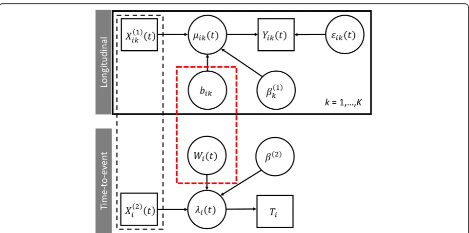
shared random effects joint model. A graphical represen-tation of this model is shown in Fig. 1. Joint models might also fall under the umbrellas of pattern-mixture models or selection models depending on the factorization of the joint distribution of event time and longitudinal data [31, 32]. Furthermore, modelling approaches might also fall under the umbrellas of joint latent class models [33], semiparametric [34], and fully parametric models [35]. We note also that the topic of missing values in lon-gitudinal data analyses has its own literature [36]. In the MVJM literature, focus has mainly been towards shared random effects models. We review the different submo-dels, including distributional assumptions and correlation structures, latent association structures, estimation tech-niques, software implementations, and give clinical exam-ples of application.
Results
Longitudinal data submodel
The choice of model for the longitudinal outcome data will depend on the type of data measured (continuous,
ordinal, discrete). Although in the development and application of MVJMs they are often restricted to the
simple case of continuous outcomes only [17, 19–21,
37–53], it is conceivable that multiple outcomes might be a mixture of different outcome types. For example, in Rizopoulos and Ghosh [29], GFR and haematocrit were both continuous measures, whereas proteinuria was recorded as a binary outcome. More recent modelling approaches developed have incorporated combinations of different outcome types [4, 18, 29, 54–65]. Other models have considered multivariate binary [66], ordinal [67, 68], and continuous [0,1]-bounded data [44, 45, 47, 53]. Thiébaut et al. [41] and Guedj et al. [52] both proposed a model for multiple continuous outcomes, but also allowed for left-censoring, which is a pertinent issue with biomarker measurements as they can fall below the minimum detec-tion level.
Model
For continuous longitudinal outcomes, the Laird and Ware [1] linear mixed model (LMM) with independent
and identically normally distributed within-subject
measurement errors is ubiquitous. However, this distri-butional assumption can be sensitive to outlier observa-tions and heavy-tailed data, which has prompted robust modelling considerations in the univariate framework [69]. Despite this, it has translated into only limited model innovation in the MVJM framework, with Tang and Tang [49] considering using the multivariate
skew-Fig. 1Graphical representation of a joint model of a time-to-event submodel andK-multivariate longitudinal outcomes submodel. Square boxes
denote observed data; circles denote unobserved (including random) terms. The black-dashed box indicates that covariates can be shared between both submodels. The red-dashed box indicates that the processWi(t) and the random effects,bi, are correlated, which gives rise to the joint
normal distribution. The robustness of model estimates to misspecification of errors, error structures, and mag-nitude of errors, has been examined through several simulation studies [40, 43, 49, 50]. Dantan et al. [44] and Proust-Lima et al. [45, 57] considered a model for [0, 1]-bounded continuous data using the Beta transformation link function, as it is parsimonious and offers very flex-ible shapes. This, however, might require a preliminary rescaling of the markers. Liu and Li [47] and Hatfield et al. [53] also considered data on the [0, 1] interval, but in-stead used zero-one inflated and ‘zero-augmented’ beta regression models, respectively. Guedj et al. [52] pro-posed a completely different approach by modelling multivariate continuous biomarkers using a mechanistic model based on a system of nonlinear ordinary differen-tial equations.
For binary and count data, the standard model is the GLMM. This model has been regularly used in the MVJM framework [4, 18, 29, 54–56, 58, 60–63, 66, 70]. Moreover, this can be extended to multivariate data of different outcome types (e.g. a combination of continu-ous and binary measures) with correlation induced by modelling the random effects together. Huang et al. [66] considered a logistic regression model for binary out-come data, with a logistic regression model for the un-observed latent variable and a linear pairwise odds-ratio model for the association between marginal probabilities. Models for ordinal data have been considered, including the proportional odds model [18, 54, 55, 64, 67], cumu-lative probit model [57], partial proportional odds model [68], and the continuation ratio mixed model [56, 59].
Random effects distributions
In the univariate joint model framework, it has been re-ported that inferences are generally robust to misspecifi-cation of random effects [71, 72]. However, in the MVJM framework the dimension of these random ef-fects might be greater, potentially amplifying the impact of misspecification on parameter estimates and standard errors. In general, the ubiquitous normality assumption might be too restrictive to capture individual-level vari-ation [49]. Nonetheless, multivariate normal distribu-tions are the standard modelling choice for random effects in the longitudinal submodel. Several simulation studies have generated data under misspecified random effects [43, 49, 60, 68]. Pantazis and Touloumi [43] ex-plored misspecification by fitting their proposed model [40] to data simulated under a range of heavy tailed, skewed, and mixture distributions. They concluded that fixed effect parameter estimates were quite robust to misspecification with the exception of those in the time-to-event submodel, but standard errors may be underes-timated for heavily skewed distributions. These findings were in agreement with those found by Li et al. [68].
Xu et al. [58] explored the sensitivity of the parameter estimates to a multivariatet-distribution for the random effects. Tang and Tang [60] investigated the effect of misspecification on their semiparametric model by simu-lating data with random effects drawn independently from uniform and relocated Gamma distributions. Song et al. [38] simulated random effects from a bimodal nor-mal mixture distribution to confirm the robustness of the semiparametric estimator; whereas Rizopoulos and Ghosh [29] simulated random effects from a three-component normal mixture model to confirm the ro-bustness of the Dirichlet process prior formulation.
To avoid misspecification, it can be advantageous to semiparametrically model the random effects. In the Bayesian paradigm, extended from the univariate frame-work [73], a Dirichlet process has been used to specify the random effects prior distribution [29, 49, 60]. The subject-specific random effects were assumed to be inde-pendently and identically distributed according to some unknown density function, which is modelled by the Dirichlet prior [74]. Song et al. [38] treated the random effects as nuisance parameters, for which a set of esti-mating equations were deduced based on a derived suffi-cient statistic. Li et al. [68] also proposed a method whereby the distributions of the assumed zero-mean random effects could be left completely unspecified and estimated entirely non-parametrically by exploiting the vertex-exchange method.
Discrete random effects confer an advantage in model estimation by replacing (possibly high-dimensional) nu-merical integration by summations that are more man-ageable. Bartolucci and Farcomeni [61] introduced two discrete random effects: one that follows a single first-order latent Markov chain distribution, and a second time-constant latent variable to account for unobserved heterogeneity. Huang et al. [66] also used independent discrete random effects to account for association be-tween events and longitudinal outcomes.
Correlation structure
multivariate normally with latent-class specific mean and an unstructured covariance matrix multiplied by a (latent) class-specific proportionality parameter. Musoro et al. [17] considered two types of random effects in the
multivariate longitudinal submodel: the standard
subject-specific random effects modelled by a multivari-ate normal distribution, and basis-outcome-specific ran-dom effects for the thin-plate spline used to model time, modelled according to independent normal distributions with basis-outcome specific variances. Li et al. [68] and Choi et al. [65] factorised the random effects asbik=Γkbi,
which reduces the dimension of random effects. For large K, Hatfield et al. [53] also discussed alternative simpler correlation structures for the random effects.
Although correlation between the multiple longitu-dinal outcomes can be modelled through the subject-specific random effects, it can alternatively be mod-elled through correlated error terms [19, 20, 38, 39, 42, 49, 60, 70]. Using the notation from (2) assuming a multivariate LMM with normal errors and multiple outcomes recorded according to a single measure-ment schedule, we have
Yik tij ¼ Xð Þik1 tij βkð Þ1 þ Zik tij bikþ εijk:
Let alsoεij⋅= (εijT1, …,εijKT )Tdenote the vector of errors
for thek-th outcome. Xu and Zeger [58] considered the
approach of correlated subject-specific random effects; namely
εijk∼Nð0;σ2kÞ; and bi∼Nvð0;ΨÞ;
whereσk2is an outcome-specific variance term, andΨis
a (v×v)-covariance matrix capturing the correlation be-tween markers and repeated measures. Chi and Ibrahim
[42] on the other hand considered the approach of
cor-related error terms; namely:
εij:∼NKð0; ΣÞ; and bik∼Nvkð0; ΨkÞ;
whereΣ is a covariance matrix that captures the
associ-ation between longitudinal outcomes measured at the
same time, and Ψk is a covariance matrix that captures
the association between the random effects for the k-th
outcome (with the vectorbikof lengthvk). Chi and
Ibra-him noted that their model allows for dependence be-tween repeated measures and correlation bebe-tween longitudinal outcomes to be considered separately, whereas in the Xu and Zeger model the different correl-ation types are conflated. Notwithstanding the inferential benefit, the latter model requires additional covariance parameters be estimated, which increases the computa-tional challenge. Interestingly, Baghfalaki et al. [64] re-placed the random effects term completely independent
of outcome k, which whilst allowing for correlation
be-tween outcomes, in general will not be biologically
plausible as subject-specific deviations will be on differ-ent scales for disparate longitudinal outcomes.
An alternative approach to model correlation between multiple longitudinal outcomes is to introduce a com-mon latent variable between the models. Ibrahim et al. [19] considered the model
Yik tij ¼ β0kþ β1kμi tij þ εijk;
where μi(tij) is the true unobserved latent variable at
time tij. For example, ifKdifferent immunological
mea-surements were recorded from a blood sample at time tij, then we might let μi(tij) denote the ‘true antibody
level’, which we cannot observe, but which we can infer
from the multivariate outcome. The model is completed by specifying the latent variable model, e.g. as in (2), and a distribution for the error terms. For example, Ibrahim et al. considered εij. ∼NK(0, Σ), and Luo [55], εijk∼
N(0,σk2). Guedj et al. [52] intrinsically accounted for
cor-relation between multiple biomarkers through the sys-tem of dependent ODE equations that models the biological system.
Within-subject autocorrelation structures, e.g. Henderson et al. [6], are not routinely considered; although Wang et al. [67] introduced a Gaussian process model for the under-lying latent variable with a power function of time model-ling the correlation. Proust-Lima et al. [57] considered the inclusion of a flexible zero-mean Gaussian autocorrelated process that admits Brownian motion and autoregressive processes as special cases. Ibrahim et al. [19], Pantazis et al. [40], and Hatfield et al. [53] noted their models could be ex-tended to autocorrelation, but at the expense of added computational burden.
In some cases, where multivariate longitudinal data has been collected, the correlation has been ignored in order to allow simpler univariate joint models to be plied. For example, Battes et al. [21] used an ad hoc ap-proach of either summing or multiplying the three repeated continuous measures (standardized according to clinical upper reference limits of the biomarker as-says), and then applying standard univariate joint models.
Time-to-event data submodel
times at a cost of loss of information and efficiency. Dan-tan et al. [44] also considered discrete time, but the model applied was relevant to continuous time also. These models do not permit premature non-informative censor-ing before the end of the study. However, Albert and Shih [46] suggested that if subjects are censored before the end of the study, then a separate precursory model could be used to impute the event times prior to application of the joint model methodology.
In practice, clinicians might not only be interested in multivariate longitudinal outcomes, but also multivariate time-to-event data. For example, Chi and Ibrahim [42] were interested in assessing whether different quality of life measures were prognostic and predictive of breast cancer progression in a drug randomised controlled trial (RCT). In addition to the multivariate longitudinal outcomes, the study monitored patients concerning two event times: overall survival and disease-free survival. Tang et al. [60], Tang and Tang [49], and Zhu et al. [70]
each proposed multiple events joint models, motivated
by the same dataset as analysed by Chi and Ibrahim
[42]. Musoro et al. [17] considered a case of multiple
recurrent events, where each patient could become repeatedly infected with one of 9 different infections. Huang et al. [66] analysed data from a complex preven-tion trial, with an interest on whether different inter-ventions were associated with times to initiation of alcohol use and tobacco use. Competing risks data have recently been considered in the context MVJMs also [56, 57, 59, 68].
Model
The Cox PH model is an attractive choice as no distribu-tional assumptions are required on the time-to-event data. In some settings, the unspecified baseline hazards function has been replaced by either a piecewise con-stant step-function for some preselected knots [18, 19, 29, 39, 47, 49, 54, 57, 59, 60, 70], or modelled using spline functions, including B-splines [4, 56], M- (and I-) splines [45, 57], and restricted cubic splines [62]. The position of knots is usually decided in advance, for ex-ample by taking quantiles (e.g. [59]), though advice is generally lacking. As an added degree of flexibility, Proust-Lima et al. [45, 57] consider class-specific (and cause-specific where applicable) baseline hazards that can be either stratified by class m= 1,…,M, i.e. λ0m(t),
or proportional by class, i.e. exp(βm)λ0(t), for some
parametersβm.
Parametric models considered in the MVJM framework include the Weibull [20, 45, 52, 53, 55, 57, 62, 64, 65], ex-ponential [20, 52, 62, 65], log-normal [40, 41, 43, 55, 64], log-logistic [55], and Gompertz [57, 62]. Hu et al. [48] used a Weibull model for imputing composite event times, but used a conditional multinomial logistic
regression model to then impute the cause type. The soft-ware package by Crowther [62] also allows for the Royston-Parmar model [75] to be fitted, which is a flexible parametric model that models the log-cumulative hazard using restricted cubic splines. For models involving multivariate event time data, standard models were applied; notably, for competing risks data the cause-specific hazards model was applied [76]. Chi and Ibrahim [42] developed a novel multivariate survival model that accommodates both zero and non-zero cure fractions, and which has a PH structure condi-tionally and marginally under certain settings. Hu et al. [48] developed an imputation approach that first imputed a composite event time, and then imputed a cause type using a conditional multinomial regression model.
The pattern-mixture model approach by Fieuws et al. [63] used the Kaplan-Meier estimator to model the failure time, which they described as prior probabil-ities, which were used in an elegant Bayes rule to cal-culate the conditional probability of failure. Models considering discrete time data have utilised a number of discrete probability models, including the probit model [46], logistic model [50], discrete time log-linear hazard models [66], truncated geometric distri-bution [50, 51, 61], and discrete proportional hazards model [50].
Frailty
Random effects are also included in some time-to-event submodels, to account for correlation between different or repeated events, where they are referred to as frailty effects when multiplicative on the hazard. Chi and Ibra-him [42] proposed a power stable law distribution to ac-count for correlation between multiple event times. Lin et al. [37] and Choi et al. [65] respectively included gamma and log-normally distributed frailty terms to allow for subject-level variability.
Association structures
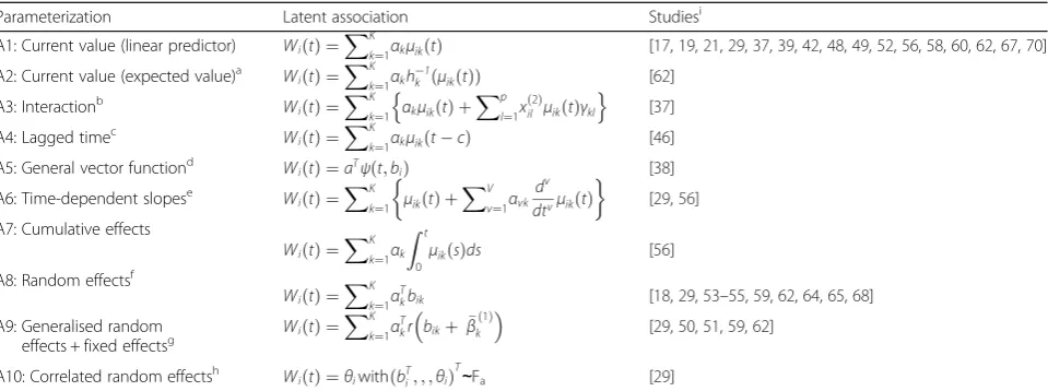
Fundamental to the joint modelling framework is the association structure between the longitudinal submo-del and the time-to-event submosubmo-del. Rationale for selecting this association structure has received rela-tively little attention. McCrink et al. [32] state that the choice of association structure should reflect the study focus, namely whether it is with respect to the time-to-event or longitudinal submodel (or both). For a discussion of different association structures for uni-variate joint models, see Rizopoulos [4]. We consider below different representations for Wi(t) applied in the MVJM
these models separately. In some cases, one might want to use different association structures for different longitu-dinal outcomes. This is a greatly overlooked modelling issue, which to the best of our knowledge, only Andrino-poulou et al. [56] and Crowther [62] have considered.
Time-dependent associations
The standard joint model assumes that risk of an event
at time t depends on the true value of the longitudinal
profile for the same time point (Table 1, A1)—the
so-called current value parameterization. The strength of the association is fully interpretable: exp(αk) is the hazard ratio
for a unit increase in μik(t), at time t. An alternative
current value parameterization is to replace the linear pre-dictor term by the expected value of the longitudinal tra-jectory function at timet,hk−1(μik(t)) (Table 1, A2), which
is of importance for correctly modelling the functional form. The current value parameterization can be extended to incorporate additional structure, including interaction terms with the covariates (Table 1, A3), which might yield more realistic inferences as it is conceivable that different associations exist for different patient subgroups. In some
cases one might posit that the risk depends not on the current value, but on a previous value, giving rise to the time-lagged values parameterization (Table 1, A4). Current value parameterizations have been used in model frame-works not compatible with (3). Chi and Ibrahim [42] adopted a novel bivariate time-to-event model whereby covariates—including a current values parameterizatio-n—are entered by a method corresponding to a canonical link in a Poisson generalized linear model. Song et al. [38] developed a model such that Wi(t) =αTψ(t, bi), for some
vector functionψ (Table 1, A5). The estimation
method-ology assumed thatψ(t,bi) could be factorised intoψ(t,bi)
=ψ(t)bi, which admits the current value parameterization
as a special case, and leads to a number of extensions in-cluding interactions with time. In cases whereψ(t,bi) does
not factorise, meaning that it is nonlinear int, the authors propose using a linear approximation method.
Derivative terms allow one to incorporate not only the current value of the true longitudinal process, but also the rate of change, which intuitively might be associated with risk of the event. For example, two patients might
have the same observed longitudinal outcome at time t,
Table 1Some association structures for joint models of time-to-event and multivariate longitudinal data
Parameterization Latent association Studiesi
A1: Current value (linear predictor) Wið Þ ¼t
XK
k¼1αkμikð Þt [17,19,21,29,37,39,42,48,49,52,56,58,60,62,67,70]
A2: Current value (expected value)a Wið Þ ¼t
XK k¼1αkh
1
k ðμikðtÞÞ [62]
A3: Interactionb Wið Þ ¼t
XK
k¼1 αkμikð Þ þt
Xp l¼1x
2
ð Þ
il μikð Þtγkl
n o
[37]
A4: Lagged timec Wið Þ ¼t
XK
k¼1αkμikðtcÞ [46]
A5: General vector functiond Wið Þ ¼t aTψðt;biÞ [38]
A6: Time-dependent slopese Wið Þ ¼t
XK
k¼1 μikð Þ þt
XV v¼1αvk
dv dtvμikð Þt
[29,56]
A7: Cumulative effects
Wið Þ ¼t
XK k¼1αk
Z t
0μikð Þsds
[56]
A8: Random effectsf
Wið Þ ¼t
XK k¼1α
T
kbik [18,29,53–55,59,62,64,65,68]
A9: Generalised random effects + fixed effectsg
Wið Þ ¼t
XK k¼1α
T
kr bikþ β̃k
1
ð Þ
[29,50,51,59,62]
A10: Correlated random effectsh WiðtÞ ¼θiwithðbTi; ; ;θiÞT∼Fa [29]
Notation:μik(t) denotes the linear predictor term of the longitudinal submodel for subjectiand outcomek;αkdenotes the association parameter for the
k-th outcome
a
hk(⋅) is the link function for thek-th outcome
b
xil(2)
denotes thel-th baseline covariates for subjecti(l= 1,…,p) with corresponding coefficient parametersγklfor each outcomek. In practice, someγkl coefficients will be set to zero
c
cis a lag time (withc= 0 returning the current value parameterization). In Albert and Shih [46], time was modelled discretely and a selection model adopted, such thatWi(tj) =∑kK= 1αkμik(tj−1)
dα
is a vector of association parameters andψ(t,bi) is a vector of time and random effects. It is assumed thatψ(t,bi) can be decomposed asψ(t,bi) =ψ(t)bi. This general parameterization admits the current value parameterization as a special case, and leads to a number of extensions including interactions with time. In cases whereψ(t,bi) does not factorise, the authors propose using an approximation method
e
αvkdenote additional association parameters for theν-th derivative (with respect to time) for thek-th longitudinal outcome mean trajectory function
fαk
denotes a vector of association parameters of same dimension as the number of random effects for each outcome. In practice, some elements ofαkmight be
forced to zero, e.g. if only random intercepts were used to link the model
g
as per the random effects parameterizationαkdenotes a vector of association parameters of same dimension as the number of random effects for each
outcome.β̃ð Þ1
k denotes the subset of coefficient parameters fromβk(1)that correspond to the random effect terms, andr(⋅) denotes a vector function. Ifr(⋅) is the identify function, then the standard random + fixed effects parameterization is returned
h
Fαdenotes a multivariate density function with parametersαto model correlation
i
but one patient’s trajectory might be rising considerably more quickly than the other patient’s. Wi(t) can
there-fore be augmented to include the current value plus the firstVderivate terms (Table 1, A6), although this model is typically only used with the first order derivatives (V
= 1), giving rise to the time-dependent slopes
parameterization. The antithesis of the time-dependent
slopes parameterization is the cumulative effects
parameterization (Table 1, A7). Here, a summary of the entire history of the longitudinal process up to timetis included in the hazard model, λi(t). This is contrary to
other association structures that relate the hazard func-tion only to features of the longitudinal model at a fixed time point.
Random effects parameterization
The above parameterizations often require numerical inte-gration, which presents a computational challenge. Simpler time-independent associations can overcome this. The ran-dom effects parameterization (Table 1, A8), which only in-cludes the time-independent random effects, is therefore frequently used in joint models. This parameterization has been used by a number of authors in various ways. In the simple case of a random-intercepts and random-slopes model for (2), the random effects represent the subject-specific deviation from the average intercept and slope fixed effect terms. Nevertheless, experts have echoed caution when attempting to use these models for inference, as com-plex longitudinal trajectory functions, such as those mod-elled by polynomials or splines, lead to non-interpretable association parameters [4, 15]. On the other hand, Jaffa et al. [50, 51] were specifically interested in the multivariate LMM slopes, so there was a clear a priori rationale for this association structure. Moreover, they noted that their model does not preclude inclusion of the random-intercepts, but demonstrated that specifying the marginal time-to-event (dropout) model is only required. Random ef-fects parameterizations are sometimes used to refer to models where the hazard is associated with random plus fixed effect terms (Table 1, A9). For example, rather than model risk as dependent onbik, one assumes it is dependent
onbikþ β
∼
k 1
ð Þ
, whereβ∼kð Þ1 is a subset ofβk(1)that correspond
to the random effects terms inbik. This model can be
gener-alised to include functions of random coefficients.
Correlated random effects and frailty
An alternative approach to specifying an association structure is not to directly include random effects com-ponents of the longitudinal submodel in the time-to-event submodel, but rather to include separate random effects in each, and specify a joint distribution for the la-tent terms (Table 1, A10). In the simplest case, one can
set Wi(t) =θi, and then jointly model (biT, θi)T.
Rizopou-los and Ghosh [29] considered such a structure, assum-ing that the joint distribution was unknown, and used a Dirichlet prior to fit the model.
Correlated random effects and error
Pantazis et al. [40], Thiébaut et al. [41], and Pantazis and Touloumi [43] assumed a log-normal distributional for the event times, i.e. log(Ti) =Xi(2)β(2)+ei, where the error
terms ei are assumed to follow a normal distribution
with mean 0 and variance σT2. The multivariate
longitu-dinal data submodel and log-normal event time submo-del were associated by assuming that (biT,ei)Tare jointly
distributed. When the random effects are multivariate normally distributed, this distribution is also multivariate normal. The covariance terms cov(bik, ei) can then
sub-sequently be used to quantify and test the strength of association.
Joint latent class models
An alternative approach to joint modelling is the use of joint latent class models (JLCMs). The assumption underlying JLCMs is that the population of subjects is heterogeneous, but consists of a number of homoge-neous latent subgroups for which the subjects share the same mean longitudinal trajectories and hazard risk. A review of JLCMs is given by Proust-Lima et al. [33]. A class-specificlatent process mixed model, which we refer to
as the latent variable model to remain consistent with
other similarly structured models, conditional on subject i
being in class m, is then specified following a standard
LMM: μiðtijkÞci¼m¼X ð1Þ
i ðtijkÞβð 1ÞþZðt
ijkÞbim. The fixed
effects coefficients can also be made class-specific [57]. The observed multivariate longitudinal data are modelled using
GLMMs or other suitablemeasurement modelsconditional
on this latent variable:hk(Yijk) =μi(tijk) +αik+εijk, for some
suitable link functions hk(⋅). If β
(1)
is forced to be class-specific, then one might introduce additional covariates with a global fixed effects coefficient vector into the meas-urement model [57]. There are two sets of random effects in this model: the subject-class effects in the latent process model, and the subject-outcome effects in the longitu-dinal data submodel. The time-to-event submodel might be modelled as a proportional hazards model,
λi(t|ci=m) = λ0m(t)exp(Xi(2)βm(2)). The class
Other
Other MVJM approaches that fall outside of the ubiqui-tous shared random effects model framework or the emerging joint latent class model framework, lead to al-ternative association structures. Fieuws et al. [63] used a pattern-mixture model approach. Here, the dependency derived from the longitudinal submodels being fitted con-ditional on the failure times. Hu et al. [48] proposed a model that incorporates some function of the history of the longitudinal data, which reduces to the current value parameterization as a special case. Bartolucci and Farcomeni [61] proposed a discrete time event-history model with a mixed latent Markov model. A flexible association structure was obtained though the introduction of two discrete latent variables: a time-varying latent variable distributed according to a finite first-order latent Markov chain, and a time-constant latent variable.
Estimation techniques
Historically, complete likelihood analysis was precluded by the inherently complex likelihood functions, necessi-tating so-called two-stage models [9, 10]. However, these models have been shown to lead to biased results [77]. A number of estimation approaches have been considered for MVJMs, building on the methodological develop-ments in the univariate joint model literature [5, 78].
Frequentist model estimation
The expectation-maximisation (EM) algorithm [79] was the original estimation approach for joint-likelihood uni-variate joint models [5, 6], and therefore continues to be employed in a number of MVJM approaches [37, 40, 43, 61, 68]. At the M-step, maximization was routinely im-plemented using both closed-form estimators and the Newton-Raphson algorithm. Some noteworthy exten-sions included the one-step-late algorithm [37] and re-stricted iterative generalized least squares [40, 43]. The E-step was typically implemented using numerical integra-tion, including Gaussian quadrature (e.g. [adaptive] Gauss-Hermite), although Monte Carlo integration [37], exten-sions of the forward-and-backwards recursion method [61], and exploitations of multivariate normal and truncated nor-mal distributions [40, 43], were also implemented. Full maximum likelihood estimation can also be implemented directly by Newtonian-like approaches. These include the Marquardt algorithm [41, 44, 45, 57], Newton-Raphson algorithm [62], and robust variance-scoring algorithm [52]. Huang et al. [66] used automatic differentiation—a numer-ical technique for simultaneously evaluating a function and its derivatives—with a Newton-Raphson algorithm, which was purportedly faster than the EM algorithm.
For estimation methods based on likelihood maximization, evaluating an approximated inverse observation matrix at the maximum likelihood estimate is a standard
approach [37, 41, 45, 52, 61, 62, 66] of calculating standard errors. Semiparametric time-to-event models have been noted to result in underestimation of param-eter standard errors [80] in the univariate joint model framework, and can be unfeasible as the information matrix increases with sample size. One approach to overcome this is the bootstrap method, which has been adopted in MVJM approaches [46, 68]. Pantazis et al. [40] and Pantazis and Touloumi [43] estimated stand-ard errors by refitting the model with multiply imputed data for censored survival times, which is quicker than conventional EM algorithm approaches.
Bayesian model estimation
Other estimation approaches
Song et al. [38] extended the semiparametric conditional score estimator for the parameters in the hazard rela-tionship, as proposed by Tsiatis and Davidian [14] in the univariate framework, which treats the random effects as nuisance parameters, and a set of estimating equa-tions are deduced based on a derived sufficient statistic. Parameter standard errors were subsequently estimated using a sandwich matrix estimator. Li et al. [68] employed a non-trivial extension of a method proposed by Tsonka et al. [82] in order to estimate the model pa-rameters and zero-mean random effects distribution using a modified vertex-exchange method algorithm in conjunc-tion with an expectaconjunc-tion-maximizaconjunc-tion algorithm. Hu et al. [48] circumvented the classical joint modelling frame-work by proposing a multiple imputation algorithm using either a fully conditional specification or MCMC proach, such that simple and transparent statistical ap-proaches can be separately applied to the complete data. Rubin’s rule [83] could then be used to account for the additional uncertainty in standard errors from imputation. Albert and Shih [46] proposed a novel two-stage regres-sion calibration approach. In the first stage, conditional on each subject’s event time, complete longitudinal data were simulated for each subject using normal approximations. Multivariate longitudinal models were then estimated using the approach of Fieuws and Verbeke [84], which fits all bivariate models and averages over the duplicate par-ameter estimates. This method is advantageous as it en-ables one to consider high-dimensional data, which would otherwise present numerical challenges or be computa-tionally infeasible. Following this, an estimator was pro-posed for the subject-specific random effects, allowing for estimates of the mean longitudinal trajectories at each discrete time point for each subject to be obtained. In the second stage, a regression-calibration approach was then used to estimate the discrete time-to-event model parame-ters. The resulting parameter estimates were averaged over repeated simulations of the model-fitting algorithm. Stand-ard errors were estimated using the bootstrap method.
Fieuws et al. [63] adopted a pattern-mixture model esti-mation approach, whereby multivariate longitudinal models
are estimated—separately for those who experience and
those who do not experience the event—again using the
proposed approach of Fieuws and Verbeke [84] described above. Bayes’rule was then used to estimate the failure time distribution conditional on the longitudinal profiles, with a non-parametric survival distribution acting as the prior distribution.
Software
The adoption of joint models has been slow [15]. Among the many reasons for this includes the historically limited availability of software specific to joint models. Recently
packages for mainstream statistical software, including R (R Foundation for Statistical Computing, Vienna, Austria) [24, 27], SAS (SAS Institute, Cary, NC) [26], Stata (Stata-Corp LP, College Station, TX) [22], and WinBUGS (MRC Biostatistics Unit, Cambridge, UK) [23], have allowed researchers to exploit joint modelling. How-ever, these have been limited to univariate data. Many articles describing developments or applications of joint models involving multivariate longitudinal data have re-ported some details about the software used to fit the joint models.
R
Brown et al. [39] compiled their flexible B-spline model for multiple longitudinal biomarkers and time-to-event outcome (with current value association parameterization) into an R package, sjmsoft, available from the author’s website: http://faculty.washington.edu/elizab/software.html [Accessed: 25 January 2016]. Battes et al. [21] used the R package JM [27], which fits univariate joint models, by re-ducing the multivariate longitudinal data to a univariate outcome through ad hoc techniques. R has also been used as an interface to execute JAGS [85] and WinBUGS/ OpenBUGS programs [47, 53, 56, 65]. Andrinopoulou et al. [59] implemented their model using two separate soft-ware packages, one of which was R, with the code available from the authors upon request. Tang et al. [60] reported their Bayesian models were fitted using R and Matlab (The MathWorks Inc., Natick, MA), with code available from the authors upon request. Albert and Shih [46] fitted the bivariate longitudinal models using code presented else-where [86]. Bartolucci and Farcomeni [61] published R code as a supplemental file for their event-history exten-sion Markov model, which depends on compiled Fortran routines.
BUGS & JAGS
Stata
It has recently been announced that the next version re-lease of the Stata package stjm [22, 87] will allow for multivariate longitudinal outcomes. The current version implements maximum likelihood estimation of univariate joint models with a number of different parametric time-to-event models. In addition, stjm can jointly model differ-ent outcome types, differdiffer-ent association structures, and different random effects covariance matrix structures, alongside extensive optimization control settings, thus giving the user immense flexibility. A number of post-estimation options are available, including residual cal-culation and prediction. Pantazis et al. [40] also report that a Stata program is available (on request from the authors) for fitting their bivariate MVJM.
Fortran
Fortran has been used in several MVJM studies [19, 44, 57, 61]. Of particular interest is the HETMIXSURV (version 2) program available from: http://www.is ped.u-bordeaux.fr/BIOSTAT [Accessed: 11 April 2006]. This Fortran 90 parallel program implements max-imum likelihood estimation of the multivariate JLCM proposed by Proust-Lima et al. [57], in addition to other related models, which permits different outcome types and submodels. The R package lcmm [28] has similar capabilities, but does not currently permit multivariate longitudinal data in the JLCM framework. Dantan et al. [44] also fitted a JLCM using Fortran 90, and note the code is available on request. Ibrahim et al. [19] also report code is available for fitting their MVJM and multivariateL-statistic from the authors’website.
Other
SAS has been implemented in the MVJM literature, with direct reference to the procedure NLMIXED [20, 50, 51, 63], but without making the code avail-able. Song et al. implemented their conditional score method using C++ [38], and Li et al. [68] fitted their bivariate ordinal model with competing risks data using C. In both cases, the code is available from the respective authors upon request. Matlab was used by Lin et al. [37] to run the one-step-ahead EM algorithm (code not pro-vided), and by Tang et al. [60] to implement an MCMC al-gorithm for a Bayesian MVJM (code available on request from the authors). Huang et al. [66] developed an S-Plus (Insightful Corporation, Seattle, WA) library model, AD09, to implement the automatic differential method that enables direct maximization of the MVJM likelihood func-tion. In addition to a Stata program, Pantazis et al. also re-ported that MLn (Centre for Multilevel Modelling, University of Bristol, UK) macros are available from the authors for fitting their bivariate MVJM.
Clinical examples
Most methodological developments in the MVJM frame-work have been motivated by real-world clinical studies. Applications have been in the disease areas of HIV/AIDS [16, 38–41, 43, 52], lung disease [65, 68], cancer [19, 37, 42, 49, 53, 60, 70], cardiovascular disease [21, 56, 59, 67], neurodegenerative disease [18, 45, 54, 55, 57], renal dis-ease [17, 29, 48, 50, 51, 63], hepatic disdis-ease [46, 61], mental health [58, 66], and cognitive studies [20, 44]. We illustrate three examples below.
Parkinson’s disease drug trial
Parkinson’s disease is a chronic progressive neurodegen-erative disorder. Luo and Wang [18] reported data from a clinical trial of 800 patients randomized in a 2x2 fac-torial design to receive double-placebo, tocopherol, dep-renyl, or tocopherol with deprenyl. The latter two groups formed the treatment group, whilst the former two defined the placebo group. To investigate the effect of tocopherol in slowing the progression of Parkinson’s dis-ease, 3 longitudinal outcomes were recorded that describe progression: 1 continuous and 2 ordinal measuring differ-ent facets of the disease. A substantial number of patidiffer-ents (376/800) failed to complete the measurement schedule (10 measurements over a 24-month follow-up period), due to deterioration and were treated with levodopa therapy. The time to initiation of levodopa therapy was the study end-point. It was shown that patients with shorter follow-up had worse progression measurements on average; therefore, a multivariate joint model was required to account for the informative dropout. For the multivariate longitudinal data, a multilevel item-response theory model was used, with centre effects included to account for the cluster-trial de-sign. A piecewise constant proportional hazards regression model was used for the time-to-event data, with a shared (centre-specific and subject-specific) random effects associ-ation structure (Table 1, A8). Based on multiple model comparison methods, a random effects parameterization without centre-level effects was optimal. This model indi-cated a non-significant effect of tocopherol on disease pro-gression rate and on the hazard of levodopa therapy initiation when compared to placebo. However, the associ-ation parameters were strongly significant, indicating that patients with worse disease severity and faster disease pro-gression had an increased hazard of levodopa therapy initi-ation. This data was also previously analysed by Luo [55] and He and Luo [54] without consideration of the centre effects, and in the former case under different parametric time-to-event models.
Heart valve replacement observational study
283 patients who survived aortic valve or root replace-ment with an allograft valve. During the routine clinical follow-up appointments, two echocardiographic measuments were recorded: valve gradient (continuous) and re-gurgitation (ordinal). Physiologically, increased gradient or regurgitation indicates deterioration of valve performance, which could lead to either death or necessitate reopera-tion—both events of interest. To investigate the effects of these parameters on the hazard of adverse events, a MVJM was proposed for the bivariate longitudinal data and a competing risks model was assumed for the event times. A LMM with B-spline functional form was used to model the non-linear gradient trajectory, and a continu-ation ratio mixed effects model for the regurgitcontinu-ation data. A simple LMM for aortic gradient was considered, but re-sulted in an inferior model fit. A cause-specific event-time model with piecewise constant baseline hazards was used to model the competing risks data, with a random effects (+ fixed effects) association structure (Table 1, A9). The association between the longitudinal measurements and events are presented in the form of graphical plots to fa-cilitate interpretation, as the B-spline parameters are not straightforwardly interpretable. Andrinopoulou et al. [56] reanalysed this data with the purpose of calculating dy-namic predictions. Furthermore, they extended the model to consider several different association structures, with subsequent predictions combined using Bayesian model averaging in order to account for model structure uncertainty.
Cancer drug trial
Lin et al. [37] reanalysed data from a placebo-controlled randomized trial to establish whether supplemental
beta-carotene reduces recurrence of the primary
tumours in patients cured from a recent early-stage head and neck cancer. The primary endpoint was all-cause mortality, with 63 subjects dying during follow-up. During the trial, blood samples were taken from 264 patients at baseline, 3-months, 1-year, and annually thereafter until 5-years total follow-up was attained. Two continuous
bio-markers—both plasma nutrient concentrations—were of
interest: lycopene and lutein + zeaxanthin. Previous uni-variate studies had demonstrated that increased biomarker concentrations were associated with reduced mortality. Interest here was specifically on whether both biomarkers were simultaneously associated with mortality. To investi-gate this, a MVJM was developed with LMMs used to model the biomarkers, and a Cox PH model to model the time to death, with association modelled using an inter-action parameterization (Table 1, A3). Additionally, a gamma-distributed subject-level frailty term was included to capture over-dispersion. It was found that the effect of lutein + zeaxanthin was diminished when both biomarkers were included, and moreover the sign was opposite to that
of the univariate joint model. By exploring the correlation between the biomarkers, the authors suggested that the ef-fect of lutein + zeaxanthin on all-cause mortality appeared to be mediated only through the association with lycopene. Lin et al. also demonstrated the necessity of joint model-ling by fitting (1) a separate event time model with base-line biomarker concentrations; (2) a time-varying covariate Cox model (equivalent to a last observation carried-forward model); and (3) a two-stage joint model, and juxtaposing each to the fitted MVJM.
Discussion
The case for use of joint models has been made in the univariate data framework [3]. Similarly in the MVJM literature, several studies have demonstrated the poten-tial bias from ignoring the correlation between the out-comes by comparing joint models to separately fitted submodels in simulation analyses [18, 40, 42, 47, 54, 55]. With an increased focus on personalised medicine, the need to implement models that account for multiple longitudinal outcomes is necessary. Despite this, joint models have predominantly focused on univariate data. A consequence of this has been researchers fitting mul-tiple separate univariate joint models [88], which is ineffi-cient and can affect inferences [37]. Here we have presented an overview of MVJM literature. The models developed in the literature showcase broad classes of lon-gitudinal and time-to-event data and countless association structures, with bespoke models often developed to meet the demands of the clinical data at hand. A small number of models have even considered simultaneously multivari-ate longitudinal data and multivarimultivari-ate time-to-event joint models [17, 42, 48, 49, 56, 59, 60, 66, 68, 70].
The extension from univariate data modelling to multivariate data modelling is, in principle, straightfor-ward [4]. The main barrier to applied researchers is the lack of readily available software that can implement multivariate joint model estimation approaches; this is despite an emergence of software relevant to univariate joint models. The main limitation to statisticians is the herent computational challenge that arises from the in-creasing dimensionality of the random effects component. Despite many multivariate models being presented in full generality, computational power, limits in numerical estimation, (effective) sample size, and clinical data availability will, unavoidably in practice, preclude analyses involving large dimensions. Of the MVJM methodologies encountered to-date, bivariate data is the most commonly encountered during application [19, 20, 37–41, 43, 48, 50, 53, 56, 57, 59, 61, 64, 68], followed by trivariate data [18, 21, 29, 44–47, 51, 58, 66]. A few articles have considered 4 longitudinal outcomes [17, 42, 49, 54, 55, 60, 63, 70]. Jaffa et al. [51] explored converge properties of their MVJM for up to 10 longitu-dinal outcomes, and reported good performance. It was also noted that the model should straightforwardly ex-tended to higher dimensions. Of all the studies involving multiple event types or competing risks, all were limited to the bivariate case/two competing risk events, with the exception of one study [17], which considered 9 separate recurrent events along with 4 longitudinal biomarkers. However, in the latter case it was reported that a sin-gle joint model could not actually be fitted due to computational limitations, with the authors opting in-stead to fit multiple pairwise models.
The flexibility of a model to be applied to a given dataset will depend on the ability to include complex functional forms and covariate adjustment options within the submodels. Complex functional forms, whilst perhaps better capturing non-linear
trajector-ies in the longitudinal submodel that may be
observed in biological data, increase computational requirements to fit as the dimensions of the random effects increases. Notwithstanding these issues, some have developed models which includes complex smoothing functions within the multivariate frame-work, including B-splines [39, 59], natural cubic splines [29, 56, 62], fractional polynomials [62], P-splines [49], thin-plate P-splines [17], I-P-splines [57], and parametric non-linear functions [43]. Albert and Shih [46] also noted that their approach could be extended to nonlinear models with an additional ap-proximation. The mechanistic model proposed by Guedj et al. [52] is able to model complex dynamics of biomarkers by virtue of the complex system of differential equations specified, which captures knowledge of actual biological processes.
Conclusions and Recommendations
Gould et al. [15] concluded that it was going to be a challenge to encourage stakeholders to adopt joint models. This challenge is further exacerbated when multivariate longitudinal data are incorporated. How-ever, as demonstrated in this review there is a solid
methodological foundation to implement these
methods. We have also observed the early phase of infiltration into the non-statistical biomedical literature [16, 20, 21], which highlights the potential of the MVJM framework. For MVJMs to be integrated into the applied biostatistician’s tool belt, further developments are re-quired, including:
Development of statistical software capable of fitting of MVJMs. Univariate joint models have seen a surge in software development, which includes wider integration with multivariate event-time data; however, lack of software for multivariate longitudinal data will preclude their use by the vast majority of applied statisticians.
Reporting of the maximum dimension limits for multiple longitudinal outcomes. Whilst many models are presented in full generality, computational limitations will preclude large numbers of random effects, and therefore large numbers of
biomarkers. Currently, little is understood about this with the exception of short commentaries by Jaffa et al. [51] and Musoro et al. [17].
Guidance on the underlying model types, distributional assumptions, and choice of association structure. Despite methodological developments, a coherent and flexible modelling framework that encapsulates the general
multivariate joint model is lacking, which precludes penetration into the biomedical arena due to a lack of understanding.
Development of model diagnostics and selection devices compatible with the MVJM framework. A number of useful ancillary statistical tools have been recently presented, however clarity and
demonstration of their suitability, as well as integration into the aforementioned software developments, are required.
Study design guidance, including but not limited to: sample size and power calculations; selection of appropriate latent association structures; applicability of models according to different intra- and inter-patient measurement protocols, and outcome types; surrogacy; and dynamic prediction.
Additional file
Additional file 1: Table S1.Goodness-of-fit tests, model diagnostics,
comparison instruments, and other model assessment tools. (DOCX 162 kb)
Acknowledgements
We thank the Medical Research Council (MRC) for funding GLH’s salary. The MRC had no influence in the design, collection, analysis, or interpretation of data; the writing of the manuscript; or the decision to submit the manuscript for publication.
Funding
This research was funded by Medical Research Council (MRC) grant MR/M013227/1.
Availability of data and materials
Not applicable. No datasets were used in this study.
Authors’contributions
RKD conceived the intellectual idea. GLH, PP, AJ and RKD designed the study. GLH wrote the manuscript. All authors reviewed drafts of the manuscript, offered interpretation and critical comment, and approved the final version.
Competing interests
The authors declare that they have no competing interests.
Consent for publication
Not applicable.
Ethics approval and consent to participate
Not applicable.
Author details
1Department of Biostatistics, University of Liverpool, Waterhouse Building, 1-5
Brownlow Street, Liverpool L69 3GL, UK.2Department of Mathematics, Physics and Electrical Engineering, Northumbria University, Ellison Place, Newcastle upon Tyne NE1 8ST, UK.
Received: 19 May 2016 Accepted: 12 August 2016
References
1. Laird NM, Ware JH. Random-effects models for longitudinal data. Biometrics. 1982;38:963–74.
2. Cox DR. Regression models and life-tables. J R Stat Soc Ser B Stat Methodol. 1972;34:187–220.
3. Ibrahim JG, Chu H, Chen LM. Basic concepts and methods for joint models of longitudinal and survival data. J Clin Oncol. 2010;28:2796–801. 4. Rizopoulos D. Joint Models for Longitudinal and Time-to-Event Data, with
Applications in R. Boca Raton: Chapman & Hall/CRC; 2012.
5. Wulfsohn MS, Tsiatis AA. A joint model for survival and longitudinal data measured with error. Biometrics. 1997;53:330–9.
6. Henderson R, Diggle PJ, Dobson A. Joint modelling of longitudinal measurements and event time data. Biostatistics. 2000;1:465–80. 7. Asar O, Ritchie J, Kalra P, Diggle PJ. Joint modelling of repeated
measurement and time-to-event data: an introductory tutorial. Int. J. Epidemiol. 2015; 1–11.
8. Dupuy J-F, Mesbah M. Joint modeling of event time and nonignorable missing longitudinal data. Lifetime Data Anal. 2002;8:99–115.
9. Self S, Pawitan Y. Modeling a marker of disease progression and onset of disease. In: Jewell NP, Dietz K, Farewell VT, editors. AIDS Epidemiol. Methodol Issues. Boston: Birkhauser; 1992.
10. Tsiatis AA, DeGruttola V, Wulfsohn MS. Modeling the relationship of survival to longitudinal data measured with error - applications to survival and CD4 counts in patients with AIDS. J Am Stat Assoc. 1995;90:27–37.
11. Hogan JW, Laird NM. Increasing efficiency from censored survival data by using random effects to model longitudinal covariates. Stat Methods Med Res. 1998;7:28–48.
12. Rizopoulos D, Hatfield LA, Carlin BP, Takkenberg JJM. Combining dynamic predictions from joint models for longitudinal and time-to-event data using Bayesian model averaging. 2013.
13. Hogan JW, Laird NM. Model-based approaches to analysing incomplete longitudinal and failure time data. Stat Med. 1997;16:259–72.
14. Tsiatis AA, Davidian M. Joint modeling of longitudinal and time-to-event data: an overview. Stat Sin. 2004;14:809–34.
15. Gould AL, Boye ME, Crowther MJ, Ibrahim JG, Quartey G, Micallef S, Bois FY. Joint modeling of survival and longitudinal non-survival data: current methods and issues. Report of the DIA Bayesian joint modeling working group. Stat Med. 2015;34:2181–95.
16. Touloumi G, Pantazis N, Babiker AG, Walker SA, Katsarou O, Karafoulidou A, Hatzakis A, Porter K. Differences in HIV RNA levels before the initiation of antiretroviral therapy among 1864 individuals with known HIV-1 seroconversion dates. AIDS. 2004;18:1697–705.
17. Musoro JZ, Geskus RB, Zwinderman AH. A joint model for repeated events of different types and multiple longitudinal outcomes with application to a follow-up study of patients after kidney transplant. Biometrical J. 2014;57:185–200. 18. Luo S, Wang J. Bayesian hierarchical model for multiple repeated measures
and survival data: an application to Parkinson’s disease. Stat Med. 2014;33:4279–91.
19. Ibrahim JG, Chen M-H, Sinha D. Bayesian methods for joint modeling of longitudinal and survival data with applications to cancer vaccine trials. Stat Sin. 2004;14:863–83.
20. Ghisletta P. Application of a joint multivariate longitudinal-survival analysis to examine the terminal decline hypothesis in the Swiss Interdisciplinary Longitudinal Study on the Oldest Old. J Gerontol B Psychol Sci Soc Sci. 2008;63:185–P192.
21. Battes LC, Caliskan K, Rizopoulos D, Constantinescu AA, Robertus JL, Akkerhuis M, Manintveld OC, Boersma E, Kardys I. Repeated measurements of NT-pro-B-type natriuretic peptide, troponin T or C-reactive protein do not predict future allograft rejection in heart transplant recipients. Transplantation. 2015;99:580–5. 22. Crowther MJ, Abrams KR, Lambert PC. Joint modeling of longitudinal and
survival data. Stata J. 2013;13:165–84.
23. Guo X, Carlin BP. Separate and joint modeling of longitudinal and event time data using standard computer packages. Am Stat. 2004;58:16–24. 24. Philipson P, Sousa I, Diggle PJ, Williamson PR, Kolamunnage-Dona R,
Henderson R. Package“joineR”[Internet]. R Foundation for Statistical Computing; 2012. Available from: https://cran.r-project.org/package=joineR. 25. Rizopoulos D. The R Package JMbayes for fitting joint models for longitudinal
and time-to-event data using MCMC.arXiv Prepr.2014; arXiv:1404. 26. Zhang D, Chen M-H, Ibrahim JG, Boye ME, Shen W. JMFit: a SAS macro for
joint models of longitudinal and survival data. J Stat Softw. 2009;30:1–3. 27. Rizopoulos D. JM: an R package for the joint modelling of longitudinal and
time-to-event data. J Stat Softw. 2010;35:1–33.
28. Proust-Lima C, Philipps V, Liquet B. Estimation of latent class linear mixed models: the new package lcmm.arXiv Prepr.[Internet] 2015; Available from: http://arxiv.org/pdf/1503.00890.pdf.
29. Rizopoulos D, Ghosh P. A Bayesian semiparametric multivariate joint model for multiple longitudinal outcomes and a time-to-event. Stat Med. 2011;30:1366–80.
30. Verbeke G, Fieuws S, Molenberghs G, Davidian M. The analysis of multivariate longitudinal data: A review. Stat Methods Med Res. 2012;23:42–59. 31. Sousa I. A review on joint modelling of longitudinal measurements and
time-to-event. Revstat Stat J. 2011;9:57–81.
32. McCrink LM, Marshall AH, Cairns KJ. Advances in joint modelling: A review of recent developments with application to the survival of end stage renal disease patients. Int Stat Rev. 2013;81:249–69.
33. Proust-Lima C, Sene M, Taylor JMG, Jacqmin-Gadda H. Joint latent class models for longitudinal and time-to-event data: a review. Stat Methods Med Res. 2012;23:74–90.
34. Scharfstein DO, Rotnitzky A, Robins JM. Adjusting for nonignorable drop-out using semiparametric nonresponse models. J Am Stat Assoc. 1999;94:1096–120. 35. Diggle PJ, Sousa I, Chetwynd AG. Joint modelling of repeated
measurements and time-to-event outcomes: the fourth Armitage lecture. Stat Med. 2008;27:2981–98.
36. Little RJA. Modeling the drop-out mechanism in repeated-measures studies. J. Am. Stat. Assoc. 1995. 1112–1121.
37. Lin H, McCulloch CE, Mayne ST. Maximum likelihood estimation in the joint analysis of time-to-event and multiple longitudinal variables. Stat Med. 2002;21:2369–82.