Comparing classification methods for diffuse reflectance spectra to improve tissue specific laser surgery

(1)

R E S E A R C H A R T I C L E

Open Access

Comparing classification methods for diffuse

reflectance spectra to improve tissue specific

laser surgery

Alexander Engelhardt

1

, Rajesh Kanawade

4

, Christian Knipfer

2

, Matthias Schmid

3

, Florian Stelzle

2

and Werner Adler

1*

Abstract

Background: In the field of oral and maxillofacial surgery, newly developed laser scalpels have multiple advantages over traditional metal scalpels. However, they lack haptic feedback. This is dangerous near e.g. nerve tissue, which has to be preserved during surgery. One solution to this problem is to train an algorithm that analyzes the reflected light spectra during surgery and can classify these spectra into different tissue types, in order to ultimately send a warning or temporarily switch off the laser when critical tissue is about to be ablated. Various machine learning algorithms are available for this task, but a detailed analysis is needed to assess the most appropriate algorithm.

Methods: In this study, a small data set is used to simulate many larger data sets according to a multivariate Gaussian distribution. Various machine learning algorithms are then trained and evaluated on these data sets. The algorithms’ performance is subsequently evaluated and compared by averaged confusion matrices and ultimately by boxplots of misclassification rates. The results are validated on the smaller, experimental data set.

Results: Most classifiers have a median misclassification rate below 0.25 in the simulated data. The most notable performance was observed for the Penalized Discriminant Analysis, with a misclassifiaction rate of 0.00 in the simulated data, and an average misclassification rate of 0.02 in a 10-fold cross validation on the original data. Conclusion: The results suggest a Penalized Discriminant Analysis is the most promising approach, most probably because it considers the functional, correlated nature of the reflectance spectra.

The results of this study improve the accuracy of real-time tissue discrimination and are an essential step towards improving the safety of oral laser surgery.

Keywords: Laser surgery, Reflectance spectroscopy, Machine learning, Penalized discriminant analysis

Background

Oral and maxillofacial surgery is a field where precise cuts with minimal operative trauma are of particular interest. Laser scalpels are able to operate much more precisely than metal scalpels. The development of laser surgery has brought forward a new method of performing surgery which reduces the risk of infection that arises when intro-ducing a metal scalpel in the patient’s body. By using a laser scalpel instead, this source of infection risk is

*Correspondence: [email protected]

1Department of Medical Informatics, Biometry and Epidemiology, Friedrich-Alexander University Erlangen-Nuremberg, Waldstrasse 6, 91054 Erlangen, Germany

Full list of author information is available at the end of the article

nearly eliminated, because no foreign body is inserted into the patient’s tissue. Postoperative healing time has been shown to decrease as well [1]. However, this technology also introduces a new problem: When using a traditional metal scalpel, surgeons can feel if they are about to cut a different type of tissue such as, a nerve—this is called hap-tic feedback—and are thus able to work around that cru-cial tissue. Preserving this tissue is of utmost importance, as irreparable nerve damage is one of the most serious side-effects of surgery. Especially in oral and maxillofacial surgery, situations arise where the complex anatomy in the head and neck region predestinates risks for certain kinds of surgeries. As an example, removing the parotid gland

(2)

can be a dangerous procedure as branches of the facial nerve run directly through the gland [2].

Laser scalpels, however, cannot provide haptic feed-back. For this reason, it is necessary to develop alternative methods to detect what type of tissue (e.g. fat, nerve, blood vessels) is being operated on during a surgery. One possible way, applied in this study, is to illuminate the region at and near the scalpel’s current position, and to measure the reflected light spectra. These spectra are given as smooth real-valued functions over a certain wave-length range, and are measured at discrete wavelenghts.

Data of this type is called functional data [3]. When

these spectra are measured in between pulses of the laser scalpel, one can then classify them and find out what tissue is about to be ablated. Finally, this can then be assembled into an algorithm that detects when the laser is about to damage critical tissue and emits a warning sig-nal to the surgeon or temporarily shuts off the laser as an automatic feedback mechanism.

Spectroscopy

For the purpose of tissue diagnostics, two popular meth-ods of spectroscopy, diffuse reflectance spectroscopy and autofluorescence spectroscopy, are available [4,5]. The

most widely used method uses autofluorescence

spec-troscopyto derive a tissue’s characteristics.

When a tissue sample is illuminated with light of spe-cific wavelengths, certain molecules called fluorophores (including amino acids, vitamins and lipids) absorb the light’s energy and subsequently emit light themselves, this time of lower energy, i.e. longer wavelengths. The concen-tration of some fluorophores changes in different tissue types, thus altering the resulting autofluorescence spectra and enabling tissue discrimination.

This study makes use ofdiffuse reflectance spectroscopy, which exploits the differences in absorption and scattering properties of various tissue types. The tissue is illuminated with white light, and a spectrometer then measures the degree of single and multiple backscattering.

The question which method is preferrable has no con-crete answer as of now. In a breast cancer detection study, Breslin et al. [5] found that autofluorescence spectroscopy is the superior method for discriminating benign from malignant breast tissue. De Veld et al. [4] however found that the analysis of diffuse reflectance spectra and aut-ofluorescence spectra performed equally well when dif-ferentiating oral lesions from healthy tissue, but diffuse reflectance spectra were better for discriminating benign from malignant lesions.

One might conclude that the two methods perform sim-ilarly in cancer detection tasks. However, Douplik et al. [6] showed that autofluorescence spectra are altered under laser ablation conditions, suggesting that another method

of spectroscopy might be more viable in a laser surgery setting.

Existing work

Previous, related studies [2,7-9] that developed a tis-sue detection algorithm compared the total misclassi-fication error, i.e. the ratio of falsely classified obser-vations to all obserobser-vations, as well as the pairwise ROC curves [10], which plot the false positive rate (_{false positives}false positives₊_{true negatives}, equal to 1 minus the specificity and ranging from 0 to 1) on thex-axis vs. the true positive rate (_{false negatives}true positives₊_{true positives}, equal to the sensitivity and ranging from 0 to 1) on they-axis. Because an ROC curve an only compare two tissue types at a time, one has to use pairwise curves, one for each tissue pair. Lastly, the pair-wise area under the ROC curve (AUC), which ranges from 0.5 for random guessing to 1.0 for a perfect classification, was compared.

Stelzle et al. [2,7] used ex-vivo pig heads to measure and classify the diffuse reflectance spectra of hard and soft tissue types, namely skin, muscle, mucosa, subcuta-neous fat, salivary gland, bone, and nerve tissue. They found that almost all tissue pairs could be differentiated with high sensitivity and specificity. Many tissue pairs could be differentiated with sensitivities and specificities of around 90%. Some sensitivities and specificities were slightly lower, but the results still show the feasibility of remote tissue differentiation. One of the problems that persist in these two studies is that measurements were taken ex-vivo, i.e. from dead tissue. The fact that blood flow to this tissue had stopped before measurements were taken implies that measurements of in-vivo tissue will dif-fer slightly, depending on the additional light absorption and scattering properties of blood occuring in live tissue.

In a follow-up study, Stelzle et al. [8] took on the above mentioned problem of ex-vivo tissue alterations. The authors classified the diffuse reflectance spectra of four soft tissue types (skin, fat, muscle, nerve) of live rats. This study achieved an AUC and a sensitivity as well as specificity of 1.00 for all tissue pairs except skin/fat. These results may suggest that, due to the additional occurence of blood in live tissue, classification perfor-mance is improved under in-vivo conditions.

(3)

All of the mentioned studies reach high sensitivities and specificities, concluding that a tissue differentiation by dif-fuse reflectance spectroscopy is feasible, even in live tissue and under laser ablation conditions.

However, all of the previously listed work used the same method of analysis: The dimension of the measured spec-tra was reduced by a Principal Component Analysis (PCA) [11], and the PC scores were subsequently classified by a Linear Discriminant Analysis (LDA) [12].

Moreover, the data in the four above-mentioned cases came from a relatively small number of specimen, where each animal has been measured many times. This resulted in a large sample size, but highly correlated spectra within animals, due to the repeated measurements.

Purpose of this study

The objective of this study is to extend the existing work in two ways: Firstly, the problem of the repeated, cor-related measurements is tackled by averaging out the repeated spectra within each animal. Because the variance of the spectra within each animal is much smaller than the variance between animals, this procedure reduces the amount of data without reducing the amount of informa-tion much, and furthermore removes a possible down-ward bias when estimating the covariance matrices for each tissue type. Afterwards, new spectra are simulated by estimating mean vectors and covariance matrices for each tissue class separately, and using these estimates to simulate new spectra according to multivariate Gaussian distributions. Secondly, the study’s main objective is to apply a series of classification algorithms to the simulated data, and find out if other classification methods have a better prediction strength than the previously applied LDA.

The insights acquired from this study can be used in further research and suggest a set of algorithms to con-centrate on for subsequent studies.

Methods

Data acquisition and preprocessing

Data acquisition

The data consist of diffuse reflectance spectra measured at a discrete set of wavelengths, taken from different tissue types of a set of ex-vivo pig heads. The initial data set used in this study is a merged data frame, combined from the data sets used in Stelzle et al. [2,7].

Measurements were taken from twelve dissected pig heads obtained from a slaughterhouse. For each pig head, eight tissue types were dissected, from each of which six spots were selected to take reflectance spectra from. Finally, 30 measurements per spot were made. The many repetitions were taken because once a tissue sample is readily lying under the spectrometer, additional measure-ments are done quickly and cheaply.

Thus, in total, the complete data consisted of 12 ani-mals· 8 tissue types · 6 spots · 30 repetitions = 17280 diffuse reflectance spectra. The spectra were measured at 1150 discrete wavelengths between 350 nm and 650 nm, in steps of around 0.26 nm. The tissues were illumi-nated with a pulsed Xenon lamp, and the reflected spectra were measured with a backscattering probe that trans-ferred the measurements to a spectrometer. Refer to Stelzle et al. [7] for further details on the experimental set up.

Preprocessing

To bring the data into a structure that is in agreement with the prerequisites for simulation, the data was thinned out by averaging over the repetitions and spots. This proce-dure was justified by looking at 30 measurements of each spot and tissue type, which showed only minimal varia-tion, and 6 measurements of each animal and tissue type at its different spots, which show almost exclusively only a constant vertical shift.

The averaging was done first and foremost to elimi-nate redundant information in the data. Secondly, it was believed that keeping the repetitions would result in a too small estimate for the covariance matrices within each tis-sue class, because the data essentially contained 30 copies of each spectrum. By making sure that each spectrum in the final data set belongs to a different animal, it can be assumed that the subsequent simulation of new spectra generates spectra of new animals instead of new spots.

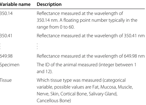
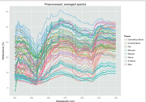
The preprocessed data set contained 96 observations (8 tissue types·12 animals) of 1154 columns, described in Table 1 and shown in Figure 1.

Simulation of new spectra

Since the previous studies were carried out with many repeated measurements of a small number of specimen, many of the measurements were highly correlated, and the

Table 1 A description of the columns in the data

Variable name Description

350.14 Reflectance measured at the wavelength of 350.14 nm. A floating point number typically in the range from 0 to 60.

350.41 Reflectance measured at the wavelength of 350.41 nm .

. .

. . .

649.98 Reflectance measured at the wavelength of 649.98 nm Specimen The ID of the animal measured (integer between 1

and 12).

(4)

0 10 20 30 40 50

350 400 450 500 550 600 650

Wavelength (nm)

Reflectance (%)

Tissue

Cancellous Bone

Cortical Bone

Fat

Mucosa

Muscle

Nerve

S.Gland

Skin

Preprocessed, averaged spectra

Figure 1All 96 spectra, 8 tissue types for each of the 12 animals, after preprocessing has taken place.This is the data set with which the simulation has been carried out. Each of the spectra is actually an average over six spots and 30 repetitions, i.e. 180 of the spectra of the original data set have been averaged into one line of this figure.

authors remarked that the sample size was actually rather small, considering the degree of redundancy in the data set.

For that reason, the data set was first shrunk by aver-aging out the repetitions, and subsequently enlarged via simulation. The simulation created spectra that can be

interpreted as measurements from new animals rather

than additional repetitions of the same animal.

After preprocessing, the remaining data set consisted of

N = 96 spectra, each belonging to one ofC = 8

tis-sue types. The number of spectra in each of theCtissue classes is denoted bync, c∈ 1,. . .,C, and is constant in this data set,nc=12∀c.

Simulation procedure

The simulation was conducted by using the following procedure:

First, split the data frame of the spectra (denoted byX) intoC=8 subsets, one for each tissue typec. Denote the resulting matrices of reflectance spectra byXc ∈ Rnc×p. Assume in each of the C tissue classes c ∈ 1,. . .,C,

each one of thencspectra follows ap-dimensional multi-variate normal distribution with meanμcand covariance matrixc,

xj∼Np(μc,c), j=1,. . .,nc.

One can then obtain simple parameter estimators μˆc andˆcfor every classcseparately:

ˆ

μc= 1

nc

⎛ ⎜ ⎝

nc

i=1xi1 .. .

nc

i=1xip

⎞ ⎟

⎠ (1)

ˆ

c= 1

nc−1

X_cXc (2)

We can subsequently use the obtained estimators to simulatemcadditional observations in each classc:

x∗_j ∼Np(μˆc,ˆc) , j=1,. . .,mc,

(5)

The estimation data sets

Using the estimated meansμˆc and covariancesˆc, new data was simulated to obtain a distribution of error rates. We generated 1000 data sets of 800 observations (mc = 100) each. These data sets were used to train classification algorithms and generate boxplots of their misclassifica-tion rates, and to compute confusion matrices to allow for more detailed insights in where misclassification occurs.

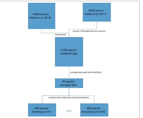
Figure 2 summarizes the data manipulation process. For the subsequent analyses, the original 96 spectra were neglected for simplicity; only simulated spectra were considered.

Dimension reduction with Principal Component Analysis (PCA)

Because the measured spectra consist of many highly correlated input variables which can lead to instable

parameter estimates, a PCA [11] was applied as a method of dimensionality reduction.

To allow a comparison between using a PCA and using the original spectra, the classification algorithms were each carried out first with the original spectra, and subse-quently with only a number of PC scores.

The computation of the principal components relies heavily on the (sample) covariance matrixof the dataX, which is the row-wise matrix composed of then observa-tionsxi. The k-th principal component is given byzk =

α

kx, whereαk is the eigenvector of corresponding to thek-th largest eigenvalueλkof.

The idea of a PCA is to use a small numberq pof

principal components that still explain a sufficient pro-portion of the total variance, thus reducing the number of input variables while losing only a minimal amount of available information.

10800 spectra Stelzle et al. (2010)

8640 spectra Stelzle et al. (2011)

17280 spectra combined data

96 spectra averaged data

800 spectra bootstrap set #1

800 spectra bootstrap set #1000 remove 2160 duplicate nerve spectra

average away spots and repetitions

simulate with multivariate normal distribution concatenate

(6)

To choose the number q of principal components for further analyses, a multitude of methods is avail-able. In this study, the average eigenvalue criterion was applied because it is an objective, computationally low-cost method which has shown good results according to Valle et al. [13]. With the average eigenvalue criterion, one selects all PCs with an associated eigenvalue greater than the average eigenvalue of all PCs.

Classification methods

The simulation and analyses were carried out with the open programming environment R, version 3.0.0 [14]. The following additional packages were used:

• For linear discriminant analysis (LDA) and quadratic discriminant analysis (QDA): TheMASSpackage [15].

• For penalized discriminant analysis (PDA): Themda package [16].

• For Random Forests: TherandomForestpackage [17].

• For classification and regression trees (CART): The rpartpackage [18].

• For Neural Networks: Thennetpackage [15].

• Fork-nearest-neighbor: Theclasspackage [15].

• For the graphics: Thereshapeandggplot2 packages [19,20].

Where possible, each classification algorithm was exe-cuted with both the original spectra as well as the PC scores. For some classifiers, one of the methods was either impossible or nonsensical:

• For LDA and QDA, highly correlated covariates (as is the case for discretized functions) lead to unstable estimates. For that reason, only PC scores were analyzed with LDA and QDA.

• PDA has its strength in the case of many correlated covariates. It thus makes little sense to analyze a set of PC scores with that algorithm, which is why only the spectra were considered for PDA.

The classification algorithms used in this study are described only briefly here. Some of the algorithms can be run out-of-the-box, whereas others depend on some tun-ing parameters orhyperparameters, which influence the course of action of the algorithm. Where necessary, these tuning parameters are described, as well. Refer to Hastie et al. [12] for an extensive description of all algorithms discussed here.

k-nearest-neighbor

Ak-nearest-neighbor classifier [21] takes a new observa-tion vector x∗, and finds itsk nearest neighbors in the training sample. The definition of closest point is sub-ject to some chosen distance metric, most commonly

the euclidean distance, which is defined as d(u,v) =

k

l=1(ul−vl)2for two vectorsuandv. The predicted class for x∗ is then the majority vote of the response variable of the nearest neighbors.

Thek-nearest-neighbor algorithm has only one hyper-parameter, namelyk.

Linear discriminant analysis (LDA)

Linear discriminant analysis [22] is based on imposing a multivariate Gaussian mixture model upon the training data i.e. it assumes:

• A class probability πcfor each classc, subject to C

c=1πc=1.

• In each classcthe input dataxifollow a multivarate Gaussian distribution:

f(x|Y =c)= 1 (2π)p/2_|_c_|1/2

exp

−1

2(x−μc)

−1

c (x−μc)

.

• Linear (as opposed to quadratic) discriminant analysis assumes the covariance matrices within all classes are equal, i.e.c=∀c.

After estimating theπc,μcandfrom the training data set T, the decision rule can be described with a set of

discriminant functions

δc(x∗)=

x∗−1μc− 1 2μ

c−1μc+log(πc).

LDA owes its name to the fact that these discriminant functions are linear in x∗. The fitting function is then

ˆ

Y(x∗)=argmax_cδc(x∗).

Quadratic discriminant analysis (QDA)

In some situations (the simulation in this study is an exam-ple), the covariance matricescare not equal throughout

all classes. In that case, a QDA [22] is an appropriate solution. The discriminant functionδc(x)has a quadratic form, and the decision boundaries between two classes

c1 andc2 are described by quadratic equations {x : δc1

(x)=δc2(x)}. In particular, the discriminant functions are defined by

δc

x∗= −1

2log|c| − 1 2(x

∗₋_μ

c)−c1

x∗−μc

+logπc,

and are thus quadratic inx∗.

Penalized discriminant analysis (PDA)

(7)

Mathematically, many correlated covariables will result in a singular, i.e. non-invertible covariance matrix , thus making the classification very instable or even infeasible. Hastie et al. [23] replace by a regularized

version, + λ, where is a roughness-penalizing

matrix andλis a smoothing parameter that adjusts the amount of smoothing. The classification then proceeds much like an LDA, but with the penalized covariance matrix.

The choice of determines the type of penalization

used. Common choices are a second-order difference structure that effectively penalizes second derivatives, or a simpler choice of = λIp that results in a penaliza-tion similar to ridge regression [24]. We chose the latter matrix,=λIp, for regularization.

Classification trees

Classification trees [12] work by partitioning the covari-ate space into rectangles and fit simple models (mostly a constant) in each rectangle. The gradual

partition-ing can be visualized through a decision tree, that

yields a path along the tree resulting in a constant, i.e. a predicted response (or an above-mentioned sim-ple model) for every new observation. Different meth-ods are available, for example the CART and C4.5 algorithms.

This analysis used CART trees, which are restricted to binary splits at each splitpoint and uses the Gini index as an impurity measure.

To control when the tree stops growing and the model is considered as finished, many hyperparameters can be used. One hyperparameter limits the depth of the tree to some maximum number. Furthermore, one can deter-mine the minimum number of observations that must exist in a node for another split to be attempted, and/or the minimum number of observations in any terminal leaf node. Alternatively, one can set a minimum factor by which the lack of fit has to be decreased in order to execute the next split.

This procedure, however, might stop a tree too early, when e.g. the next split is of little importance, but a subsequent split could lead to a large increase in classi-fication accuracy. Thus, one usually employs a strategy called pruning, where first a large tree is grown, and subsequently splits of little importance removed, keeping possible better splits further down the tree. A

hyperpa-rameter α controls how good a split has to be so that

it is kept in the final, pruned tree. In the case ofα=0 the solution is the full tree, for α=1 a degenerated

tree with zero splits results. Since α is the minimum

factor by which the lack of fit must be decreased in order for the next split to be executed, it makes sense

to only search for α in the low end of the possible

interval [ 0, 1].

Random forests

Random forests [25] are anensemble method, construct-ing a large number of simple classification trees to obtain a majority vote for the predicted response class. They work because simple trees are high-variance yet unbiased methods, and the “averaging” reduces that high variance.

In short, a random forest is constructed by drawing

B bootstrap samples from the training data and fitting a tree to each of them, randomly selecting a subset of covariates at each splitpoint. The predicted class for

new observations is then the majority vote of the B

fitted trees.

Hyperparameters for random forests include the stop-ping criteria for each tree, explained above, as well as

the total number B of trees to grow, and the number

of variables that are randomly sampled as candidates at each split. The last parameter is the most influential one regarding the final goodness of fit.

Neural networks

A neural network for classification [12] is (for the most common case of one hidden layer) a two-stage classifica-tion model, consisting of ahidden layer, which in turn is made up ofMso-called hidden units (or neurons)Zm = σ(α_X₎_{, where}_X_{is the covariate matrix. The output layer} gc(T), where T = βZ, is the second step in the two-stage model. The predicted class for an observation is then the classcwith the largest respective value ofgc(T). Neu-ral networks are inspired by the workings of neurons in a brain, where they get their name from. The sequen-tial interconnection between the covariates, the neurons and the output layer models the interconnected nature of neurons.

When considering only single layer networks, the main parameter is the numberMof hidden units in this layer. Furthermore, the activation functionσ(v)can be speci-fied, although it is mostly the sigmoid function,σ(v) =

1/(1+e−v). Finally, the output functiongc(T)can be spec-ified, but for classification purposes, it is most commonly the softmax function,gc(T)= e

Tc

C

γ=1eTγ .

Hyperparameter selection

Some classifiers depend on additional hyperparameters which have to be set before the algorithm is run. This section describes which paramters were tuned and how they were chosen.

(8)

(50% of the observations) and one test set (the other 50% of the observations) was carried out. The best hyper-parameter was then determined by comparing the total misclassification rate in the test set for a reasonable set of different values for the hyperparameters and choosing the parameter with the lowest respective misclassification rate.

The following hyperparameters were determined:

• Fork-nearest-neighbor classification, the parameter kwas determined by splitting the data into training and test data, computing a fit for allk∈ {1,. . ., 10}, and choosing for subsequent analysis the value fork which resulted in the smallest test set error.

• For random forests, the parametermtry, i.e. the number of covariates randomly selected for each tree split, was searched for using the proceduretuneRF in therandomForest-package. It compares different values ofmtrywith their respective out-of-bag errors, but does not try every possible value formtry, instead it multiplies or dividesmtry by a constant factor (2 in this study) at each iteration.

• For classification trees, the complexity parameterα was searched for by first growing a large tree with α=10−6_{. This tree contains a table of}

cross-validation errors for several values ofαlarger than10−6_{, and the optimal value of}_α_{was extracted} from this table and used as the pruning complexity parameter.

• For neural networks, the number of hidden units in the middle layer was searched for from 1 to 4 in the case of spectra, and from 1 to 10 in the case of PC scores. The range for number of units was limited in the case of spectra for computational reasons.

• For PDA, the smoothing parameterλwas searched for from10i, i= −6,. . ., 3.

Performance evaluation

All algorithms were applied on each of the 1000 estima-tion data sets. The classifiers were trained on a sample set (50% of each data set, i.e. 400 of the 800 observations), and their performance was subsequently evaluated on an independent test set (the remaining 400 observations).

Distribution estimation of the misclassification rate

The variation of the misclassification rate was of central interest in this study. The 1000 estimation data sets were generated for that reason. The classification algorithms were applied to the training data of each of these data sets and subsequently evaluated on the test data.

The misclassification rate is the percentage of observa-tions for which a wrong class was predicted. Denoting the covariates (i.e. the spectra) in the test set byxi, and their

respective tissue type by yi, the misclassification rate is defined by

1

n #{i: Yˆ(xi)=yi}

for a test set withnobservations.

To estimate a distribution of the misclassification rate, for each of the 1000 data sets the classifiers were trained and tested, yielding a sample of misclassification rates. These samples were used to create boxplots of the mis-classification rates to allow for a better performance judgment.

Averaged confusion matrices

To obtain insights into the specific type of mistakes made in the classification, an average of the confusion matrices

of the 1000 simulated data sets was computed. ItsC =

8 rows andC = 8 columns are the specific tissue types, and the percentages show what ratio of tissues of typec

get classified into groupd. These insights can be helpful to find out what type of tissues are especially difficult to discriminate.

Results

Principal component analysis

For all of the the 1000 estimation data sets, the aver-age eigenvalue criterion selected 6 principal components. Therefore, classification of PC scores was always carried out with 6 covariates.

Averaged confusion matrices

For each of the algorithms, 1000 confusion matrices were generated, one for each of the estimation data sets. Shown are the averages for each investigated algorithm. The con-fusion matrices show the actual tissue types yi in the columns, and the classified tissue typesYˆ(xi)in the rows. Therefore, (only) the row percentages sum up to 1.

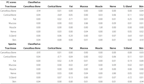
k-nearest-neighbors

Fork-nearest neighbors, the PC scores of fat and the sali-vary gland get confused most often (for 20 and 25 percent of all their respective observations).

Looking at the original spectra, cortical bone and the salivary gland get misclassified most often, both of them into similar tissue types (muscle, nerve, and fat, as well as the respective other tissue type).

Table 2 shows the confusion matrix for this algorithm.

LDA

(9)

Table 2 The average confusion matrices for the KNN algorithm

PC scores Classified as

True tissue Cancellous Bone Cortical Bone Fat Mucosa Muscle Nerve S. Gland Skin

Cancellous Bone 0.94 0.01 0.00 0.00 0.00 0.00 0.00 0.04

Cortical Bone 0.04 0.69 0.05 0.00 0.03 0.06 0.11 0.02

Fat 0.00 0.02 0.71 0.01 0.00 0.01 0.25 0.00

Mucosa 0.00 0.00 0.02 0.86 0.00 0.09 0.01 0.01

Muscle 0.00 0.00 0.00 0.00 1.00 0.00 0.00 0.00

Nerve 0.00 0.03 0.00 0.04 0.00 0.85 0.05 0.02

S.Gland 0.00 0.06 0.20 0.00 0.01 0.07 0.65 0.01

Skin 0.04 0.00 0.00 0.01 0.00 0.01 0.00 0.93

Spectra Classified as

True tissue Cancellous Bone Cortical Bone Fat Mucosa Muscle Nerve S.Gland Skin

Cancellous Bone 0.95 0.01 0.00 0.00 0.00 0.00 0.00 0.03

Cortical Bone 0.04 0.71 0.04 0.00 0.02 0.06 0.11 0.01

Fat 0.00 0.02 0.78 0.01 0.00 0.01 0.19 0.00

Mucosa 0.00 0.00 0.02 0.87 0.00 0.09 0.02 0.01

Muscle 0.00 0.00 0.00 0.00 1.00 0.00 0.00 0.00

Nerve 0.00 0.03 0.00 0.04 0.00 0.86 0.05 0.02

S.Gland 0.00 0.07 0.13 0.00 0.01 0.07 0.72 0.01

Skin 0.04 0.00 0.00 0.01 0.00 0.01 0.00 0.94

into cancellous bone and muscle tissue. The confusion matrix is shown in Table 3.

Neural networks

Analyzing the PC scores with neural networks, the com-mon mistake made by other classifiers, i.e. confusing the salivary gland and fat tissues, is also visible here. Cor-tical bone is again hard to classify, but seems to get misclassified into other tissues with equal frequencies.

When running a neural network on the original spectra, the confusion matrix appears as if it were produced mostly by random guessing. Only cancellous bone was recog-nized with an increased frequency of 0.40. See Table 4 for the confusion matrix.

PDA

A penalized discriminant analysis made almost no mis-takes and correctly classified nearly all of the samples in the test set. A small amount of misclassification occured but is not visible in the confusion matrices due to round-ing. This can have a number of reasons, including the nature of the simulation procedure or simply its intrin-sic advantage when dealing with functional data. The confusion matrix is shown in Table 5.

QDA

A quadratic discriminant analysis of the PC scores made almost no mistakes, merely misclassifying some cortical bone, fat, nerve, and salivary gland tissues. See Table 6 for the confusion matrix.

Table 3 The average confusion matrix for the LDA algorithm, analyzing PC scores

Cancellous Bone 0.93 0.03 0.00 0.00 0.00 0.00 0.00 0.04

Cortical Bone 0.10 0.74 0.03 0.00 0.06 0.03 0.03 0.01

Fat 0.00 0.01 0.83 0.00 0.00 0.02 0.15 0.00

Mucosa 0.00 0.05 0.00 0.93 0.00 0.02 0.00 0.00

Muscle 0.00 0.00 0.00 0.00 1.00 0.00 0.00 0.00

Nerve 0.00 0.06 0.01 0.00 0.00 0.85 0.07 0.01

S.Gland 0.00 0.01 0.09 0.00 0.00 0.01 0.89 0.00

(10)

Table 4 The average confusion matrix for the neural net algorithm

Cancellous Bone 0.92 0.04 0.00 0.00 0.01 0.00 0.00 0.03

Cortical Bone 0.07 0.78 0.04 0.01 0.02 0.04 0.03 0.02

Fat 0.00 0.04 0.81 0.01 0.00 0.03 0.11 0.00

Mucosa 0.00 0.01 0.01 0.94 0.00 0.03 0.00 0.01

Muscle 0.00 0.01 0.00 0.00 0.98 0.00 0.00 0.00

Nerve 0.01 0.04 0.02 0.02 0.00 0.86 0.04 0.01

S.Gland 0.00 0.02 0.11 0.00 0.00 0.03 0.82 0.01

Skin 0.04 0.01 0.00 0.02 0.00 0.01 0.01 0.91

Cancellous Bone 0.40 0.06 0.07 0.08 0.14 0.07 0.07 0.11

Cortical Bone 0.13 0.09 0.14 0.12 0.16 0.14 0.12 0.09

Fat 0.07 0.07 0.20 0.16 0.11 0.17 0.15 0.08

Mucosa 0.08 0.07 0.17 0.20 0.12 0.15 0.13 0.09

Muscle 0.15 0.07 0.11 0.11 0.26 0.11 0.10 0.09

Nerve 0.07 0.07 0.18 0.15 0.11 0.17 0.15 0.08

S.Gland 0.08 0.07 0.17 0.15 0.11 0.16 0.16 0.09

Skin 0.21 0.07 0.10 0.12 0.14 0.10 0.10 0.17

Random forests

Random forests make similar mistakes than other clas-sifiers when analyzing PC scores, most notably the con-fusion of fat and salivary gland. However, the overall error rate is smaller than for discriminant analyses and

k-nearest-neighbor classification.

For PC scores, the types of misclassification are sim-ilar, but the overall performance suffers noticeably. The resulting confusion matrix is shown in Table 7.

Trees

Trees have a relatively weak performance in this analysis. Analyzing the original spectra with trees show a partic-ularly weak performance. Comparing them with random

forests, one can see that the ensemble method does not result in a big improvement in discrimination of cancel-lous bone and muscle tissue, but improves the discrimi-nation of the six other tissue types. See Table 8 for the confusion matrix of this algorithm.

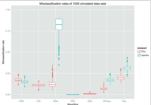
Misclassification rates

The 1000 misclassification rates per algorithm were sum-marized into quantiles. The 0% quantile is equal to the minimum, the 50% quantile is the median, and the 100% quantile is the maximum of each vector. The quantiles are shown in Table 9 and depicted as boxplots in Figure 3.

The worst performing algorithms were neural nets with original spectra and the tree algorithms, both for PC

Table 5 The average confusion matrix for the PDA algorithm, analyzing spectra

Cancellous Bone 1.00 0.00 0.00 0.00 0.00 0.00 0.00 0.00

Cortical Bone 0.00 1.00 0.00 0.00 0.00 0.00 0.00 0.00

Fat 0.00 0.00 1.00 0.00 0.00 0.00 0.00 0.00

Mucosa 0.00 0.00 0.00 1.00 0.00 0.00 0.00 0.00

Muscle 0.00 0.00 0.00 0.00 1.00 0.00 0.00 0.00

Nerve 0.00 0.00 0.00 0.00 0.00 1.00 0.00 0.00

S.Gland 0.00 0.00 0.00 0.00 0.00 0.00 1.00 0.00

(11)

Table 6 The average confusion matrix for the QDA algorithm, analyzing PC scores

Cancellous Bone 1.00 0.00 0.00 0.00 0.00 0.00 0.00 0.00

Cortical Bone 0.00 0.98 0.01 0.00 0.00 0.01 0.00 0.00

Fat 0.00 0.01 0.98 0.00 0.00 0.00 0.01 0.00

Mucosa 0.00 0.00 0.00 1.00 0.00 0.00 0.00 0.00

Muscle 0.00 0.00 0.00 0.00 1.00 0.00 0.00 0.00

Nerve 0.00 0.01 0.00 0.00 0.00 0.99 0.00 0.00

S.Gland 0.00 0.00 0.01 0.00 0.00 0.00 0.98 0.00

Skin 0.00 0.00 0.00 0.00 0.00 0.00 0.00 1.00

scores and original spectra. However, as noted above trees were not tuned because of the many available hyper-parameters, and thus might have resulted in a better performance after tuning.

The best performances were achieved by a quadratic discriminant analysis of the PC scores and a penal-ized discriminant analysis of the original spectra. Both achieve a near-perfect classification with minimal varia-tion throughout the 1000 data sets.

The remaining algorithms had a similar performance, with median error rates roughly between 10 and 20 per-cent. Random forests showed an improved performance when analyzing PC scores. Taking into consideration that there were eight tissue types, i.e. random guessing would

have resulted in a misclassification rate of 7/8, most of the algorithms perform strongly in this study.

Confirmatory cross validation on the original spectra

The simulation procedure used to generate the data was based on a multivariate normal distribution. Thus, mod-els which impose a normal distribution on the data can be overoptimistic in the classification procedure [12]. This applies to the discriminant analyses, i.e. LDA, QDA and PDA. Because these classifiers assume normal distribu-tions for each of the class densities, the discriminant analyses, and in particular QDA, which allows for dif-ferent covariance matrices c in the classes c, could show a reduction in classification performance for real,

Table 7 The average confusion matrix for the random forest algorithm

Cancellous Bone 0.97 0.02 0.00 0.00 0.00 0.01 0.00 0.00

Cortical Bone 0.02 0.87 0.02 0.00 0.02 0.02 0.02 0.02

Fat 0.00 0.01 0.89 0.00 0.00 0.02 0.08 0.00

Mucosa 0.00 0.01 0.00 0.97 0.00 0.01 0.00 0.00

Muscle 0.00 0.00 0.00 0.00 0.99 0.00 0.00 0.00

Nerve 0.01 0.03 0.02 0.00 0.00 0.90 0.03 0.00

S.Gland 0.00 0.01 0.08 0.00 0.00 0.03 0.88 0.00

Skin 0.01 0.01 0.00 0.00 0.00 0.00 0.00 0.98

Cancellous Bone 0.93 0.01 0.00 0.00 0.01 0.00 0.00 0.04

Cortical Bone 0.04 0.70 0.05 0.01 0.03 0.06 0.08 0.03

Fat 0.00 0.02 0.79 0.01 0.00 0.01 0.17 0.00

Mucosa 0.00 0.00 0.02 0.83 0.00 0.10 0.02 0.03

Muscle 0.00 0.01 0.00 0.00 0.98 0.00 0.00 0.00

Nerve 0.01 0.02 0.00 0.07 0.00 0.83 0.03 0.04

S.Gland 0.00 0.09 0.13 0.02 0.01 0.07 0.67 0.01

(12)

Table 8 The average confusion matrix for the CART (tree) algorithm

Cancellous Bone 0.89 0.05 0.01 0.01 0.02 0.01 0.00 0.01

Cortical Bone 0.05 0.68 0.08 0.05 0.03 0.05 0.03 0.04

Fat 0.00 0.06 0.73 0.01 0.00 0.05 0.14 0.01

Mucosa 0.03 0.07 0.02 0.85 0.00 0.04 0.00 0.00

Muscle 0.01 0.02 0.01 0.01 0.95 0.00 0.00 0.00

Nerve 0.04 0.07 0.06 0.03 0.00 0.74 0.05 0.00

S.Gland 0.01 0.02 0.17 0.00 0.00 0.07 0.72 0.00

Skin 0.05 0.02 0.01 0.01 0.02 0.02 0.02 0.86

Cancellous Bone 0.87 0.02 0.00 0.00 0.03 0.00 0.00 0.08

Cortical Bone 0.05 0.47 0.08 0.03 0.04 0.09 0.16 0.08

Fat 0.00 0.07 0.67 0.01 0.00 0.01 0.23 0.01

Mucosa 0.01 0.01 0.03 0.67 0.00 0.18 0.06 0.05

Muscle 0.01 0.01 0.00 0.00 0.97 0.00 0.00 0.01

Nerve 0.01 0.03 0.00 0.14 0.00 0.72 0.04 0.06

S.Gland 0.01 0.16 0.19 0.05 0.01 0.07 0.49 0.03

Skin 0.16 0.04 0.00 0.04 0.00 0.05 0.03 0.67

non-simulated data. One method of avoiding this problem might have been to carry out another simulation proce-dure, i.e. one that does not rely on a normal distribution.

To get a picture of the extent of overoptimism of the dis-criminant analyses, all of the classifiers have been applied to the original (i.e. non-simulated) 96 spectra. Since the original data cannot be arbitrarily augmented through simulation, in this case a cross validation [26] makes sense. Therefore, the data set has been split into ten groups of about equal size (six groups of ten spectra, and four groups of nine spectra). Subsequently, the training and validation procedure was applied ten times for each

algorithm, each time using nine of the ten groups as train-ing data and the remaintrain-ing group as a test data. The resulting misclassification rates for the ten groups were then averaged and are shown in Table 10 and displayed in Figure 4.

The figure shows that the linear and quadratic discrimi-nant analyses now perform similar to random forests and

k-nearest-neighbors. Untuned trees perform a bit weaker. It is interesting that a penalized discriminant analysis still performs much better than all the other algorithms, and achieves a near-perfect classification accuracy even for real data.

Table 9 Quantiles of the misclassification rates in the 1000 simulated data sets

0% 25% 50% 75% 100%

KNN PCs 0.12 0.16 0.17 0.19 0.24

KNN spectra 0.09 0.14 0.15 0.16 0.22

LDA PCs 0.05 0.10 0.11 0.12 0.16

NNet PCs 0.05 0.10 0.12 0.14 0.34

NNet spectra 0.35 0.76 0.82 0.89 0.92

PDA spectra 0.00 0.00 0.00 0.00 0.00

QDA PCs 0.00 0.01 0.01 0.01 0.03

RForest PCs 0.03 0.06 0.07 0.08 0.14

RForest spectra 0.11 0.16 0.17 0.19 0.25

Tree PCs 0.13 0.18 0.20 0.22 0.31

(13)

Figure 3Misclassification rates of the investigated algorithms for 1000 simulated data sets.For LDA and QDA, only the PC scores were analyzed, and for PDA, only the original spectra were analyzed. The results suggest that the PDA and QDA algorithms are the most appropriate classifiers for this type of problem.

Table 10 Average misclassification rates in a 10-fold cross validation

Algorithm Misclassification rate

KNN PCs 0.27

KNN spectra 0.26

LDA PCs 0.34

NNet spectra 0.98

NNet PCs 0.43

PDA spectra 0.02

QDA PCs 0.27

RForest PCs 0.27

RForest spectra 0.34

Tree PCs 0.55

Tree spectra 0.50

Discussion

When looking at the classifiers that were applied to both PC scores and original spectra, it seems that reducing the dimensionality, i.e. the amount of information, with a PCA results in a better performance for most algorithms. From the simulation study, a quadratic and a penalized discrim-inant analysis were near-perfect regarding the test-set error. Furthermore, these two classifiers showed almost no variability when repeating the analysis with 1000 data sets. However, a cross validation on the original data set showed that a QDA exhibits a large amount of overopti-mism due to the details of the simulation procedure.

Comparing the results of this study with the previous analyses of Stelzle et al. [2,7], one can see similar results for the LDA of PC scores. Small differences arise, of course, because of the different data preprocessing. A PDA seems to be a much better choice than the previously applied PCA and LDA.

(14)

0.00 0.25 0.50 0.75 1.00

KNN LDA NNet PDA QDA RForest Tree

algorithm

Misclassification r

a

te

analyzed

PCs

spectra

Average misclassification rates in the 10−fold cross validation of original 96 spectra

Figure 4A 10-fold cross validation of the original data.When analyzing non-simulated data, LDA and QDA show a weaker performance than in the simulated data sets. PDA also suffers a bit, but still achieves a very high accuracy. The random partitioning of the data into 10 folds was performed 50 times, and the resulting standard deviations over 50 repetitions are shown in the error bars.

A new sample of original data can be helpful in validating the results of this simulation study. Because the original data come from only twelve animals, the models we com-puted are probably not robust enough to be employed in a real surgery scenario. However, we believe a compar-ison study is feasible and insightful even with a smaller sample size, especially with the subsequent validation we performed. Still, it would be insightful to obtain spectra of a larger number of animals, ideally before and after laser ablation, and—barring ethical concerns—of live tissue.

The performance measure considered in this study was a simple misclassification rate, which does not consider the severity of special kinds of misclassification. Further analyses could take that fact into consideration. For exam-ple, if a laser scalpel would be disabled near nerve tissue as well as blood vessels, for the final system it would not matter much if a nerve spectrum would be classified as a blood vessel, since the laser is shut down anyway.

Similarly, a binary division of tissues into “critical” and “non-critical” might be considered for further studies.

Then, the performance measures can be extended to mea-sure precision and recall, amongst others.

It would be of interest under which circumstances mis-classification occurs. If a laser scalpel is approaching nerve tissue during a surgery, an undiscovered measurement of nerve tissue would be less problematic if the follow-ing measurement is correctly classified as nerve tissue. However, if the nerve tissue remains undiscovered even throughout repeated measurements, the tissue can be severely damaged before it is noticed. It is therefore inter-esting to find out if misclassifications occur randomly or show some repeated structure.

(15)

Extending on the previous point, a functional PCA [11], which imposes a smoothness constraint on the eigenvec-tors (thus making themeigenfunctions) can be of interest.

A similar application for these results is the case of tumor detection by spectroscopy. Tumor detection aims to classify the reflectance spectra of tissues into tumor tissue vs. normal tissue. In this case, since there is no surgery going on while the spectra have to be analyzed, time is not of concern. For that reason, other, more time-consuming methods of spectroscopy can be used. Raman spectroscopy [27] is one of these methods that could pro-vide more accurate results, but takes a greater amount of time to measure the reflectance spectra.

Conclusion

To conclude, this study confirmed the results of previous studies such as Stelzle et al. [2,7], who have found that classification of diffuse reflectance spectra of different tis-sue types is a feasible way of improving the safety of laser surgery. As an extension, in this study a QDA and a PDA turned out to be a notable improvement to the previously applied LDA. PDA has shown an equally well performance on a cross-validation on original, i.e. non-simulated data and should be considered for further studies. Additionally, functional data approaches [3] seem like another promis-ing improvement and could be investigated in further studies.

Competing interests

The authors declare that they have no competing interests.

Authors’ contributions

AE performed the statistical analyses and wrote the manuscript. WA and MS had the idea for the study and provided methodological guidance throughout the analysis. FS and CK conceived the project, performed the experiments and collected the data. RK contributed to ideas. All authors revised the manuscript and approved the final version.

Acknowledgements

We acknowledge support by Deutsche Forschungsgemeinschaft and Friedrich-Alexander-Universität Erlangen-Nürnberg (FAU) within the funding program Open Access Publishing.

Author details

1_{Department of Medical Informatics, Biometry and Epidemiology,}

Friedrich-Alexander University Erlangen-Nuremberg, Waldstrasse 6, 91054 Erlangen, Germany.2_{Department of Oral and Maxillofacial Surgery, Erlangen}

University Hospital, Glückstrasse 11, 91054 Erlangen, Germany.3Department of Medical Biometry, Informatics and Epidemiology, University of Bonn, Sigmund-Freud-Strasse 25, 53105 Bonn, Germany.4SAOT - Graduate School in Advanced Optical Technologies, Paul-Gordan-Strasse 6, 91052 Erlangen, Germany.

Received: 27 February 2014 Accepted: 9 July 2014 Published: 16 July 2014

References

1. Luomanen M:A comparative study of healing of laser and scalpel incision wounds in rat oral mucosa.Eur J Oral Sci1987,95(1):65–73. 2. Stelzle F, Zam A, Adler W, Tangermann-Gerk K, Douplik A, Nkenke E,

Schmidt M:Optical nerve detection by diffuse reflectance spectroscopy for feedback controlled oral and maxillofacial laser surgery.J Transl Med2011,9(1):20.

3. Ramsay JO:Functional Data Analysis. Hoboken: Wiley Online Library; 2006. 4. De Veld DC, Skurichina M, Witjes MJ, Duin RP, Sterenborg HJ, Roodenburg JL:Autofluorescence and diffuse reflectance spectroscopy for oral oncology.Lasers Surg Med2005,36(5):356–364.

5. Breslin TM, Xu F, Palmer GM, Zhu C, Gilchrist KW:Autofluorescence and diffuse reflectance properties of malignant and benign breast tissues.Ann Surg Oncol2004,11(1):65–70.

6. Douplik A, Zam A, Hohenstein R, Kalitzeos A, Nkenke E, Stelzle F: Limitations of cancer margin delineation by means of autofluorescence imaging under conditions of laser surgery. J Innovat Optical Health Sci2010,3(01):45–51.

7. Stelzle F, Tangermann-Gerk K, Adler W, Zam A, Schmidt M, Douplik A, Nkenke E:Diffuse reflectance spectroscopy for optical soft tissue differentiation as remote feedback control for tissue-specific laser surgery.Lasers Surg Med2010,42(4):319–325.

8. Stelzle F, Adler W, Zam A, Tangermann-Gerk K, Knipfer C, Douplik A, Schmidt M, Nkenke E:In vivo optical tissue differentiation by diffuse reflectance spectroscopy: preliminary results for tissue-specific laser surgery.Surg Innov2012. [http://sri.sagepub.com/content/early/ 2012/02/14/1553350611429692.full.pdf+html]

9. Stelzle F, Terwey I, Knipfer C, Adler W, Tangermann-Gerk K, Nkenke E, Schmidt M:The impact of laser ablation on optical soft tissue differentiation for tissue specific laser surgery-an experimental ex vivo study.J Transl Med2012,10(1):123.

10. Fawcett T:An introduction to roc analysis.Pattern Recogn Lett2006, 27(8):861–874.

11. Jolliffe I:Principal Component Analysis. Hoboken: Wiley Online Library; 2005.

12. Hastie T, Tibshirani R, Friedman J, Franklin J:The Elements of Statistical Learning: Data Mining, Inference and Prediction,vol. 27. New York: Springer; 2005: 83–85.

13. Valle S, Li W, Qin SJ:Selection of the number of principal components: the variance of the reconstruction error criterion with a comparison to other methods.Ind Eng Chem Res1999,38(11):4389–4401. 14. R Core Team:R: A Language and Environment for Statistical Computing.

Vienna: R Foundation for Statistical Computing; 2013. [http://www.R-project.org/]

15. Venables WN, Ripley BD:Modern Applied Statistics with S. 4th edn. New York: Springer; 2002. ISBN 0-387-95457-0, [http://www.stats.ox.ac.uk/pub/ MASS4]

16. Leisch F, Hornik K, Ripley BD:Mda: Mixture and flexible discriminant analysis.2013, R package version 0.4-4, [http://CRAN.R-project.org/ package=mda]

17. Liaw A, Wiener M:Classification and regression by randomforest. R News2002,2(3):18–22.

18. Therneau T, Atkinson B, Ripley B:Rpart: recursive partitioning.2013, R package version 4.1-1. [http://CRAN.R-project.org/package=rpart] 19. Wickham H:Reshaping data with the reshape package.J Stat Software

2007,21(12):1–20.

20. Wickham H:Ggplot2: Elegant Graphics for Data Analysis. New York: Springer; 2009. [http://had.co.nz/ggplot2/book]

21. Friedman JH, Baskett F, Shustek LJ:An algorithm for finding nearest neighbors.IEEE Trans Comput1975,24(10):1000–1006.

22. Friedman JH:Regularized discriminant analysis.J Am Stat Assoc1989, 84(405):165–175.

23. Hastie T, Buja A, Tibshirani R:Penalized discriminant analysis.Ann Stat 1995,23(1):73–102.

24. Yu B, Ostland M, Gong P, Pu R:Penalized discriminant analysis of in situ hyperspectral data for conifer species recognition.IEEE Trans Geosci Rem Sens1999,37(5):2569–2577.

25. Breiman L:Random forests.Mach Learn2001,45(1):5–32.

26. Efron B:Estimating the error rate of a prediction rule: improvement on cross-validation.Stat1983,78(382):316–331.

27. Kneipp K, Kneipp H, Itzkan I, Dasari RR, Feld MS:Ultrasensitive chemical analysis by raman spectroscopy.Chem Rev1999,99(10):2957–2976.

doi:10.1186/1471-2288-14-91