Mathematical simulation of thermal behavior of moving bed reactors

*

Corresponding author: [email protected] 48

Mathematical Simulation of Thermal Behavior of Moving Bed

Reactors

L. Mahmoodi 1, B. Vaferi 2*, M. Kayani 1

1

Department of Chemical Engineering, Yasouj University, Yasouj, Iran

2

Young Researchers and Elite Club, Shiraz Branch, Islamic Azad University, Shiraz, Iran

ARTICLE INFO ABSTRACT

Article history:

Received: 2016-11-01

Accepted: 2016-12-20

Temperature distribution is a key function for analyzing and optimizing the thermal behavior of various process equipment. Moving bed reactor (MBR) is one of the high-tech process equipment which tries to improve the process performance and its energy consumption by fluidizing solid particles in a base fluid. In the present study, thermal behavior of MBR has been analyzed through mathematical simulation. Good agreement between the obtained results and both experimental data and analytical solution by self-adjoint method is observed. Mathematical results confirm that the average particle temperature linearly increases across the reactor length. Fluid temperature changes in a parabolic manner, and then it changes linearly. Increasing the Biot number (Bi_Rad.) results in increasing the temperature gradient inside the particle to a maximum value, and thereafter a decreasing pattern is observed. The numerical results confirmed that the finite-difference method can be used for thermal analysis of the moving bed reactor.

Keywords:

Moving Bed Reactor Mathematical Simulation Thermal Analysis

Temperature Profiles

1.Introduction

In recent years, an increasing interest in employing the moving bed technology in chemical separation processes is observed [1-2]. It is reported that the improvement of process performance, decrease in investment and maintenance cost, and energy consumption can be achieved by moving bed configuration [1]. It is possible to transfer heat by passing the bulk material through a cooling or heating process [2].

Temperature profile, which is necessary for understanding the thermal behavior of processing equipment, can be obtained by

Iranian Journal of Chemical Engineering, Vol. 14, No. 4 (Autumn 2017) 49 method, its consistency, stability,

convergence, conservation, bounded-ness, reliability and most importantly its accuracy should be checked carefully [3-4]. Moreover, the systematic errors due to modeling, discretization, and iteration must be minimized.

For considering the heat and/or mass transfer between solid particles and fluid phases of moving bed systems, a great variety of technological applications are presented [5-6]. Bertoli analyzed heat transfer process in a moving bed using two different methodologies, namely lumped parameter model and distributed parameter one [5-6], and validated the obtained results by some experimental data [7]. In these studies, the author employed the Laplace transform method with inversion by the residue theorem to find analytical solutions to the governing equations of the considered system, and observed good agreement between the experimental data and predicted ones. By using the self-adjoint operator method, Meier et al. (2009) presented an analytical solution for thermal behavior of moving beds system with time-dependent parameters [8]. Some researchers have focused on the fluid catalytic cracking (FCC) process in a circulating fluidized bed reactor [9, 10]. In these models, the spatial variations of the process variables are considered in both distributed parameter model and lumped parameter model. Further, Valipour and Saboohi presented a mathematical model to simulate the multiple heterogeneous reactions in a moving bed of porous pellets on a reactor [11]. In another work, Valipour and Saboohi presented a model to predict flow in a cylindrical reactor in which pellets of iron ore went through a gas mixture [12]. Moreover, Belighit studied the gasifying coal using concentrated solar

radiation in a moving bed reactor from numerical point of view, and compared the obtained results with experimental data [13]. In this study, a great deal of efforts should be devoted to demonstrating the application of the finite-difference method for the solution of system of PDEs obtained from shell energy balance over the MBR. The direct solution to the differential equations of both particle and bulk fluids is one of the

advantages of the present approach.

Moreover, it can be easily used as an interpolation scheme to solve numerical advection/diffusion problems.

2. Model development

A special characteristic of the moving bed systems is the creation of enforced motion in pourable bulk solids [2, 8]. In a moving bed configuration, heat is transferred by movement of the bulk material through a cooling or heating section [5, 14]. Amount of heat transfer in moving bed systems is mainly determined by time of direct contact of the particles with the heat-transfer surface.

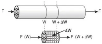
As mentioned earlier, shell energy balance methodology is employed to derive the differential equations which govern the heat transfer through MBR. The energy balance is written over a volume element of a considered system. Fig. 1 illustrates a differential volume element of the MBR in which the energy conservation law will be written over it.

50 Iranian Journal of Chemical Engineering, Vol. 14, No. 4 (Autumn 2017)

Some simplifying assumptions are considered for modeling thermal behavior of the MBR, some of the most important of which are as follows:

1. Velocities and physical properties of the fluid and the particles are constant and uniform.

2. Temperature of the reactor wall is constant.

3. Dragging gas can be considered as transparent to radiation.

4. All of the solid particles are

characterized as uniform spheres. 5. Heat diffusion in both radial and axial

directions is neglected.

6. Shape factor of radiation heat transfer (F) equals one.

7. Heat of chemical reaction is

negligible.

Amount of radiation heat flux from the reactor wall to the solid particles is calculated by the linearized Stefan-Boltzmann equation as expressed by Eq. (1).

) (

.

. Rad w p

Rad h T T

Q = − (1)

where h_Rad.=σε_pS_f(T_w2 +T_p2)(T_w +T_p).

Unsteady state energy balance of the spherical solid particle includes the Fourier equation of the heat diffusion resulting in Eq. (2) [8]:

( )

( )

( )

r t r T

r r

t r T

t t r T

D

p p

p

p ∂

∂ + ∂

∂ = ∂

∂ , , ₂ ,

1

2 2

(2)

For the fluid with convective heat transfer, accumulative, and interface heat transfer terms, the energy equation can mathematically expressed as follows [8]:

( )

( )

_[

_{( )}

_]

_[

_{( )}

_]

ps f

p p f

w w w f

f f f f

f

f a h T T w t n A h T wt T

w t w T C t

t w T

C + − − −

∂ ∂ −

= ∂ ∂

, ,

, ,

n

ρ n

ρ (3)

Required boundary and initial conditions for the above differential equations are presented

by Eqs. (4) and (7).

(

)

0 , 0

= ∂

= ∂

r t r Tp

(4)

(

)

_[

_{( )}

_]

₍

₎

w ps Rad f

ps p p

p

p h T T w t h T T

r t R r T

k = − + −

∂ = ∂

− , , _. (5)

(

)

p r t T

T , =0 = (6)

(

)

f w t T

T =0, =0 = (7)

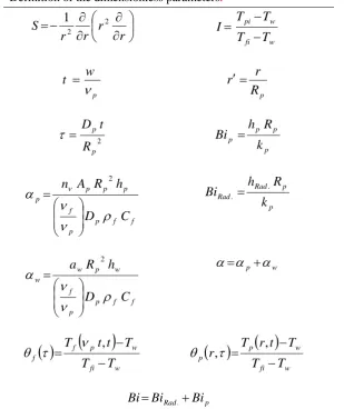
It is convenient to present the above-governing equations, initial and boundary conditions in terms of dimensionless parameters. Table 1 presents the definition of dimensionless parameters employed in this study. In this table, α_p quantifies effects of

the particles on the fluid, while α_w presents

effect of wall on the fluid, respectively. α is

the combination of both effects, B_p

represents the convective heat transfer between the particle surface and the fluid, and

r

Iranian Journal of Chemical Engineering, Vol. 14, No. 4 (Autumn 2017) 51

Table 1

Definition of the dimensionless parameters.

      ∂ ∂ ∂ ∂ − = r r r r

S 1₂ 2

w fi w pi T T T T I − − = p w t n = p R r r′=

2 p p R t D = t p p p p k R h Bi = f f p p f p p p p C D h R A n ρ n n α n         = 2 p p Rad Rad k R h Bi . = .

f f p p f w p w w C D h R a ρ n n α         = 2 w p α α α= +

( )

(

)

= n ,

t θ

( )

( )

The dimensionless forms of the governing equations, boundary and initial conditions can be mathematically expressed by Eqs. (8) and (13). p p Sθ t θ = ∂ ∂ − (8) ps p f

f _{αθ α θ}

t θ − = ∂ ∂ − (9)

(

)

(

)

∂ 1,

(11)

(

)

p ′,t =0 =

θ (12)

(

)

θf (13)

3. Numerical solution

In this study, a straightforward approach is employed to discretize the spatial domain and approximate the PDE by the ordinary differential equation (ODE) in the grid points. Thereafter, a finite-difference model (FDM) can simply be utilized to solve a set of ODEs. By employing Euler method for the time integration, it is possible to obtain Eq. (14).

(

)

T

T n

n n

n − = ∆

+ + + 1 1 1 , (14)

52 Iranian Journal of Chemical Engineering, Vol. 14, No. 4 (Autumn 2017)

4. Derivation of the discretized model

By discretizing differential equations of both fluid and particle using the finite-difference method, it is possible to convert PDE into a set of ODEs. It should be mentioned that the time and spatial derivatives are discretized

with forward and central differences, respectively.

4.1. Heat transfer equation of the particle

The discretized form of the inner nodes of heat transfer equation of particles can mathematically be expressed by Eq. (15).

(

) (

[

)

(

)

]

[

(

)

(

)

]

( )

[

(

)

(

)

]

r dt k j i k j i k j i k j i p p p p p p , , 1 , , 1 , , 1 , , 1 2 , , 1 , 1 , − − + × ′ ′ + − + + × + × − = + θ θ θ θ λ θ λ θ (15)

Herein, i represents location counter, j is time counter, and k indicates counter of experimental parameters (α_p, α_w, Bi_p,

. Rad

Bi ). dr′ and dt are location and time increments, respectively.

4.2. Heat transfer equation of the fluid

The discretized form of the dimensionless equation of fluid temperature is presented by Eq. (16).

(

)

( )

[

]

(

) (

)

f θ α θ α

θ +1, = , ×1− + ′, , × (16)

θp

(

)

temperature at the inner nodes of the spherical

particle. Interior temperature of particle equation is:

(

)

(

) (

)

[

(

)

(

)

]

( )

[

(

)

(

)

]

r d i r dt k j i k j i k j i k j i p p p p p p , , 1 , , 1 , , 1 , , 1 2 1 , , , 1 , − − + × ′ ′ + − + + + − × = + θ θ θ θ λ λ θ θ (17)

Moreover, the fluid temperature equation can be written as below:

(

)

( ) ( )

( ) (

)

p +1, =1−θ , ×α +α θ ′, ,

θ (18)

4.2.1. Stability and convergence

To obtain consistent and stable results, λ

should be as below:

4 4 1 2 2 r d dt r d dt ′ = → ≤ ′ = λ λ (19)

Location step equals 0.1, and time step will

be obtained from the above equation.

4.2.2. Boundary conditions

The first boundary condition is obtained through the forward difference method in time and space.

0 = ′

r

(

)

(

)

(

)

3 , 1 , 3 , 1 , 2 4 , 1 ,

1 j k p j k p j k

p + − + = + θ θ θ (20)

For the second boundary condition, use time and spatial derivatives with forward and

Iranian Journal of Chemical Engineering, Vol. 14, No. 4 (Autumn 2017) 53 1 = ′ r

(

)

(

)

(

)

( ) (

)

3

)

(

2

,

1

2

3

)

(

2

,

1

,

2

,

1

,

1

4

,

1

,

+

′

+

′

+

+

′

+

−

′

−

+

−

′

=

+

′

k

Bi

r

d

k

j

k

Bi

r

d

k

Bi

r

d

k

j

r

n

k

j

r

n

k

j

r

n

θ

θ

θ

θ

The experimental parameters (α , Bi_r , Bi_p,

f

T , T_p) are obtained from Lisbôa [7]. The first distant step and time step are defined for the model, and then initial condition is allocated to the nodes of the particles and fluid.

5. Results and discussion

In this section, a great deal of effort shall be devoted to validating the mathematical results with those which are obtained through

experimental measurements. Results of the finite-element method are compared with both self-adjoint method and experimental data reported by Lisbôa [7]. It is completely obvious that the model is valid and accurate enough according to the following results.

5.1. Validation of the model results

Table 5 describes the experimental values of the moving bed reactor reported by Lisbôa [7]. These experimental values are utilized to validate the numerical results of the FDM.

Table 2

Experimental conditions used in the simulation [7, 15].

( )

T_p  T_w

( )

( )

( )

( )

     C m W h_{p }

2

80.3 400.0 106.0 31.0 31.0 289.0

      C m W

h_{w 2 } F_p

(

)

f p

F F

(

)

u_p / u_f

(

)

18.99 44.0 5.6 2.67 5.178 0.9943

Table 3

Physical properties of oil shale fines [7].

) (mm dp p ε ) /

(Kj KgK

Cp ) / ( 3 m Kg p ρ ) /

(W mK

kp 348.8 0.86 961.4 2.3 1.4

In Table 4, the results of our model, those of self-adjoint method [5], and experimental data [7] are presented. It can be seen that the excellent agreement exists between our model and experimental ones.

In this section, the errors observed between models and experimental data are calculated

numerically. The absolute relative deviation (ARD %) which is defined by the following equation is employed for numerical verification of the modeling results.

54 Iranian Journal of Chemical Engineering, Vol. 14, No. 4 (Autumn 2017)

Herein, PV indicates parameter value.

Table 5 presents a comparison between accuracy of FDM and self-adjoint method in the prediction of the experimental data reported by Lisbôa for a mixture of oil shale fines and air. It is observed that the proposed model shows good predictions of the experimental data and self-adjoint method. It

can be concluded that the finite-difference method can correctly predict both experimental data and self-adjoint modeling results (analytical solution). These results confirm that the proposed FDM in this study can be used for thermal analysis of moving bed reactors.

Table 4

Comparison between the calculated and experimental temperatures of fluid and particle.

Experimental results [7] Self-adjoint method [5]

Our results

( )

T_p 

( )

T_f 

( )

T_p 

( )

T_f 

( )

T_p 

( )

T_f 

80.3 106.0

79.7 109.0

80 110

Table 5

Value of error index between the calculated and experimental results.

ARD % between self-adjoint method and experimental data

ARD % between our model and experimental data

( )

T_p 

( )

T_f 

( )

T_p 

( )

T_f 

0.75 2.83

0.37 3.77

5.2. Calculation of temperature profile

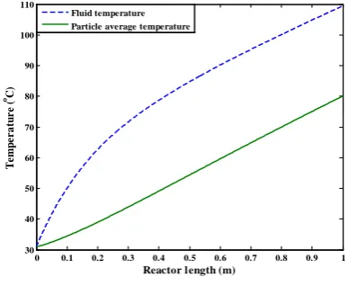
Fig. 2 illustrates the axial distribution of the fluid temperature and average particle temperature. It can be seen that the average particle temperature changes approximately linearly over the reactor length. It can be explained by the fact that the total rate of heat transfer to the particles was approximately constant along the reactor length.

Figure 2. Axial distribution of the fluid temperature and average particle temperature.

At the entry of the MBR, due to the quick heating of the fluid in relation to the particles, heat convection in the particles surface is high; however, with increasing the reactor length, the radiation heat rate in particles surface increases and heat convection decreases. Therefore, due to the greater heat capacity of the solids in comparison with the

fluid, the ratio of

T Rad

Q Q _.

(Radiant heat rate

to total heat transferred to the particles) increases with reactor length.

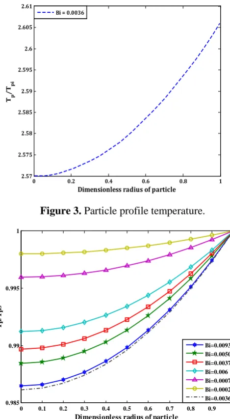
Fig. 3 presents the particle temperature profile at the entry of the moving bed reactor. It can be concluded that by increasing the

particle radius, the ratio of

pi p

T T

increases.

Fig. 4 shows temperature profile of the solid

particle under various hydrodynamic

conditions. Rearranged in the form of

0 0.1 0.2 0.3 0.4 0.5 0.6 0.7 0.8 0.9 1

30 40 50 60 70 80 90 100 110

Reactor length (m)

T

em

p

era

tu

re (

oC)

Iranian Journal of Chemical Engineering, Vol. 14, No. 4 (Autumn 2017) 55

p p Rad Rad

k R h

Bi _. = . , Biot number for radiation

heat transfer may physically be interpreted as the ratio of the internal conduction resistance to the external radiation resistance. It is illustrated that the inside temperature of the particle increases when Br is increasing,

following until reaching a maximum value

and then decreases.

This behavior may be explained by the fact that the solid particles of the MBR can become hotter than the fluid with a dragging fluid transparent to thermal radiation under certain conditions.

Figure 3. Particle profile temperature.

Figure 4. Radial profile of the particle temperature for various radiation Biot numbers at the reactor outlet.

In Fig. 5, unsteady state variation of particle temperature as a function of reactor length is illustrated. This type of information can be used for obtaining the numeric value of temperature of particle in any desired spatial

and temporal point of interest. It can be simply understood that the particle temperature gradually increases with reactor length over time.

0 0.2 0.4 0.6 0.8 1

2.57 2.575 2.58 2.585 2.59 2.595 2.6 2.605 2.61

Dimensionless radius of particle

Tp /Tpi

Bi = 0.0036

0 0.1 0.2 0.3 0.4 0.5 0.6 0.7 0.8 0.9 1

0.985 0.99 0.995 1

Dimensionless radius of particle

T

p/

T

ps

56 Iranian Journal of Chemical Engineering, Vol. 14, No. 4 (Autumn 2017) Figure 5. 3D presentation of variation of particle temperature as function of time and reactor length.

Unsteady state profile of variation of fluid temperature as as function of reactor length is depicted in Fig. 6. This figure shows that the

rate of increase of fluid temperature with reactor length is higher than its variation over time.

Figure 6. 3D presentation of variation of fluid temperature as a function of time and particle Biot number.

6. Conclusions

In this study, it was possible to employ finite-difference method to numerical analysis of the radiation and convection heat transfer to a

pneumatically conveyed mixture of solid particles, including radial dependence on fluid temperature. By comparing the numerical results of the FDM with the experimental data

0

2

4

6

8 0

0.2 0.4

0.6 0.8

1 30

40 50 60 70 80 90

Time (s) Reactor length (m)

P

a

r

ti

cl

e T

em

p

era

tu

r

e (

o C)

0 0.01

0.02 0.03

0.04

0 2 4 6 8 20

40 60 80 100 120

Time (s)

Bi

p

F

lu

id

t

em

p

era

tu

re (

Iranian Journal of Chemical Engineering, Vol. 14, No. 4 (Autumn 2017) 57 and self-adjoint method, it was concluded that

this method can be used for thermal analysis of the moving bed reactor.

The numerical results of the MBR can be summarized as follows:

(1) The average particle temperature variation is approximately linear with the reactor length, explained by the fact that the total rate of heat transferred to the particles was approximately constant along the reactor length.

(2) It can be concluded that with an increase

in particle radial, ratio

pi p

T T

increases.

(3) Temperature gradient inside the particle increases when Bi_Rad.is increasing, although other parameters are constants, and it follows until reaching a maximum value and then decreases.

Nomenclature

A surface area of single particle. Bi Biot number.

C specific heat capacity. D thermal diffusion coefficient.

f

S shape factor.

h heat transfer coefficient.

k thermal conductivity. Q heat flux.

r′ radial distance. R particle radius. T temperature.

t time.

w axial coordinate. F mass flow rate.

Subscription/Superscription

calc calculated. exp experimental.

f fluid.

i inlet.

p _particle.

w wall.

.

Rad radiative.

Greek letters

α heat diffusion coefficient.

σ Stefan–Boltzmann constant.

n kinematic viscosity.

ε emissivity.

ρ density.

∆ difference.

Abbreviations

ARD absolute relative deviation. FCC fluid catalytic reactor. FDM finite difference model. MBR moving bed reactor.

ODE ordinary differential equation. PDE partial differential equation. PV parameter value.

References

[1] Pivem, A. C. and de Lemos, M. J. S., “Laminar heat transfer in moving porous bed reactor simulated with a macroscopic two energy equation model”, Int. J. Heat. Mass. Tran., 55 (7-8), 1922 (2012).** [2] Niegsch, J., Koneke, D. and Weinspach,

P. M., “Heat transfer and flow of bulk solids in a moving bed”, Chem. Eng. Process., 33 (2), 73 (1994).

[3] Oliver, Y. P. Z., “Comparison of finite difference and finite volume methods & the development of an education tool for the fixed- bed gas adsorption problem”, M.Sc. thesis of chemical and bio-molecular engineering of national university of Singapore, Singapore, p. 37 (2010).

[4] Yip, S., Handbook of materials

modeling, 1st ed., Springer, Berlin, p. 31 (2005).

58 Iranian Journal of Chemical Engineering, Vol. 14, No. 4 (Autumn 2017)

[6] Bertoli, S. L., “Radiant and convective heat transfer on pneumatic transport of particles: An analytical study”, Int. J. Heat. Mass. Tran., 43 (13), 2345 (2000). [7] Lisbôa, A. C. L., “Transferência de calor

em leito de arrasto de xisto”, M.Sc. thesis of federal university of Rio de Janeiro, Rio de Janeiro, p. 99 (1987).

[8] Meier, H. F., Noriler, D. and Bertoli, S. L., “A solution for a heat transfer model in a moving bed through the self-adjoint operator method”, Lat. Am. Appl. Res.,

39 (4), 327 (2009).

[9] Becerril, E. L., Yescas, R. M. and Sotelo, D. S., “Effect of modeling pressure gradient in the simulation of industrial FCC risers”, Chem. Eng. J., 100 (1-3), 181 (2004).

[10]Michapolous, J., Papadokonstadakis, S.,

Arampatzis, G. and Lygeros, A.,

“Modeling of an industrial fluid catalytic cracking unit using neural networks”,

Chem. Eng. Res. Des., 79 (2), 137 (2001).

[11]Valipour, M. S. and Saboohi, Y.,

“Modeling of multiple non-catalytic gas-solid reactions in a moving bed of porous pellets based on finite volume method”,

Heat. Mass. Transfer., 43 (9), 881 (2007).

[12]Valipour, M. S. and Saboohi, Y., “Numerical investigation of non-isothermal reduction hematite using syngas: the shaft scale study”, Model. Simul. Mater. Sc., 15 (5), 487 (2007). [13]Belghit, A., Daguenet, M. and Reddy, A.,

“Heat and mass transfer in a high temperature packed moving bed subject to an external radiative source”, Chem. Eng. Sci., 55 (18), 3967 (2000).

[14]Leao, C. P. and Rodrigues, A. E., “Transient and steady-state models for

simulated moving bed processes:

Numerical solutions”, Comput. Chem. Eng.,28 (9), 1725 (2004).