Computational method based on triangular operational matrices for solving nonlinear stochastic differential equations

ISSN: 2008-6822 (electronic)

http://dx.doi.org/10.22075/ijnaa.2017.1023.1198

Computational method based on triangular

operational matrices for solving nonlinear stochastic

differential equations

Mahnaz Asgaria,b,∗, Morteza Khodabinb

a_{Department of Engineering, Abhar Branch, Islamic Azad University, Abhar, Iran} b_{Department of Mathematics, Karaj Branch, Islamic Azad University, Karaj, Iran}

(Communicated by M. Eshaghi)

Abstract

In this article, a new numerical method based on triangular functions for solving nonlinear stochastic differential equations is presented. For this, the stochastic operational matrix of triangular functions for Itˆo integral are determined. Computation of presented method is very simple and attractive. In addition, convergence analysis and numerical examples that illustrate accuracy and efficiency of the method are presented.

Keywords: Brownian motion; Itˆo integral; Nonlinear stochastic differential equation; Stochastic operational matrix; Triangular function.

2010 MSC: Primary 65C30, 60H35, 65C20; Secondary 60H20, 68U20.

1. Introduction

Mathematical formulation of real problems causes differential equations, integro-differential or partial differential equations involving stochastic excitations of a Gaussian white noise. Such problems are mathematically modeled by stochastic differential equations (SDE), or in more complicated cases, by nonlinear stochastic differential equations of the Itˆo type. Most of these equations do not have analytical solution, so it is important to find their approximate solution. In recent years, some different numerical methods for solving stochastic differential or stochastic integral equations have been presented ([12]-[9]). The topic of our study is integral form of SDE as follows

x(t) = x0+

Z t

0

k1(t, s)b(s, x(s))ds+

Z t

0

k2(t, s)σ(s, x(s))dB(s), t ∈[0 1), (1.1)

∗_{Corresponding author}

Email addresses: [email protected] (Mahnaz Asgari),[email protected](Morteza Khodabin)

where, x0 is a random variable independent of B(t), B = (B(t), t ≥ 0) is a Brownian motion and

stochastic process x is a strong solution of Eq. (1.1), it is adapted to {_zt, t ≥ 0}, furthermore, all Lebesgue,_{s and Itˆo’s integrals in Eq. (1.1) are well defined [11].}

Deb et al. in [6], proposed orthogonal triangular function (TF) sets which derived from the block pulse function (BPF) set. They presented the operational matrix for integration in TF and they established that the TF technique is more accurate than the BPF technique. The benefit of TF is that the TF representation does not need any integration to evaluate the coefficients, so it reduces a lot of computational cost. TF approximation has been used for the analysis of dynamic systems [7], integral equations ([13],[4]) and integro-differential equations [3].

In this paper, we derive stochastic operational matrices of TFs, useing them in reducing the nonlinear stochastic differential equation to a set of algebraic equations.

In Section 2, a brief review of TFs is presented. In Section 3, stochastic operational matrices of TFs are derived. Section 4 is devoted to the formulation of nonlinear SDE. In Section 5 convergence analysis of the method is discussed. In Section 6 some numerical examples are provided. Finally, Section 7 gives a brief conclusion.

2. TFs and their properties

Twom-set TFs presented by Deb et al. [6] are defined over the interval [0 T) as follows

T1i(t) =

1−t−ih

h ih≤t <(i+ 1)h, 0 elsewhere,

T2i(t) =

_t−ih

h ih≤t <(i+ 1)h, 0 elsewhere,

where, i = 0, . . . , m−1, and h = _mT. Without loss of generality, it is supposed that the interval of integration is [0 1], since any finite interval [a b] can be transformed to interval [0 1] by linear maps.

TFs, are disjoint, orthogonal, and complete [3]. We considerm-set TF vectors as

T1(t) = [T10(t), . . . , T1m−1(t)]T, T2(t) = [T20(t), . . . , T2m−1(t)]T,

and

T(t) = [T1(t), T2(t)]T.

A square integrable functionf(t) can be expanded into an m-set TF series as

f(t)'fˆ(t) =F1TT1(t) +F2TT2(t) =FTT(t), t∈[0T), (2.1) where, F1i = f(ih) and F2i =f((i+ 1)h) for i = 0, . . . , m−1. The vectors F1 and F2 are called the 1D-TF coefficient vectors and 2m-vectorF is defined as

F = [F1, F2]T.

The operational matrix for integration can be obtained as [6]

Z t

0

where,

P =

P1 P2

P1 P2

,

and

P1 = h 2       

0 1 1 . . . 1 0 0 1 . . . 1 0 0 0 . . . 1

..

. ... ... . .. ... 0 0 0 . . . 0

      

m×m

, P2 = h 2       

1 1 1 . . . 1 0 1 1 . . . 1 0 0 1 . . . 1

..

. ... ... . .. ... 0 0 0 . . . 1

      

m×m

.

It can be concluded that

T(t)TT(t)X = ˜XT(t), (2.2) and

TT(t)BT(t) = ˆBT(t), (2.3) in whichB is a 2m×2m matrix,X is a 2m-vector, ˜X =diag(X) andB is a 2mvector with elements equal to the diagonal entries ofB. In addition, the integral of f(t) can be approximated as follows:

Z t

0

f(s)ds' Z t

0

FTT(s)ds'FTP T(t).

A function of two variables,k(t, s), can be expanded with respect to TFs as follows

k(t, s)'kˆ(t, s) = TT(t)KT(s),

where K is a 2m1×2m2 coefficient matrix of TFs. For convenience, we put m1 = m2 =m. So, K

can be written as

K =

K1 K2

K3 K4

2m×2m

,

where K1, K2, K3 and K4 can be computed by sampling k(t, s) at points si and ti such that

si =ti =ih, fori= 0,1, . . . , m. So, the following approximations can be obtained (K1)ij =k(si, tj), i= 0,1, . . . , m−1, j = 0,1, . . . , m−1, (K2)ij =k(si, tj), i= 0,1, . . . , m−1, j = 1, . . . , m, (K3)ij =k(si, tj), i= 1, . . . , m, j = 0,1, . . . , m−1, (K4)ij =k(si, tj), i= 1, . . . , m, j = 1, . . . , m.

3. Stochastic operational matrix of TFs

In this section, we obtain stochastic operational matrix of TFs for the Itˆo integral. Let

I(T(t)) = Z t

0

T(s)dB(s) = Z t

0

T1(s)

T2(s)

dB(s) = Rt

0 T1(s)dB(s)

Rt

0 T2(s)dB(s)

, (3.1)

therefore, we compute R₀tT1i(s)dB(s) and Rt

0 T2i(s)dB(s). By using definition of the unit step

function we can rewrite T1i(t) and T2i(t) as follows

T1i(t) =

u(t−ih)− t−ih

h u(t−ih) +

t−(i+ 1)h

and

T2i(t) =

t−ih

h u(t−ih)−

t−(i+ 1)h

h u(t−(i+ 1)h)−u(t−(i+ 1)h) ,

so Z t

0

T1i(s)dB(s) = Z t

0

{u(s−ih)− s−ih

h u(s−ih) +

s−(i+ 1)h

h u(s−(i+ 1)h) dB(s), (3.2)

and Z t

0

T2i(s)dB(s) = Z t

0

{s−ih

h u(s−ih)−

s−(i+ 1)h

h u(s−(i+ 1)h)−u(s−(i+ 1)h) dB(s), (3.3) u(t) is the unit step function. These integrations can be divided into three cases. For the case of

t∈[0 ih), we have

Z t

0

T1i(s)dB(s) = 0, (3.4) and

Z t

0

T2i(s)dB(s) = 0. (3.5) For the case of t∈[ih (i+ 1)h),we have

Z t

0

T1i(s)dB(s) = (i+ 1) Z t

ih

dB(s)− 1

h

Z t

ih

sdB(s)

= (i+ 1)[B(t)−B(ih)]− 1

h

Z t

ih

sdB(s), (3.6) and

Z t

0

T2i(s)dB(s) = 1

h

Z t

ih

sdB(s)−i

Z t

ih

dB(s)

= 1

h

Z t

ih

sdB(s)−i[B(t)−B(ih)]. (3.7) Finally, for the case oft∈[(i+ 1)h T),we get

Z t

0

T1i(s)dB(s) = Z ih

0

T1i(s)dB(s) +

Z (i+1)h

ih

T1i(s)dB(s) + Z t

(i+1)h

T1i(s)dB(s)

=

Z (i+1)h

ih

T1i(s)dB(s) = (i+ 1)

Z (i+1)h

ih

dB(s)− 1

h

Z (i+1)h

ih

sdB(s)

= (i+ 1)[B((i+ 1)h)−B(ih)]− 1

h

sB(s)(_ihi+1)h− 1

h

Z (i+1)h

ih

B(s)ds

= 1

h

Z (i+1)h

ih

B(s)ds−B(ih), (3.8) and

Z t

0

T2i(s)dB(s) = 1

h

Z (i+1)h

ih

sdB(s)−i

Z (i+1)h

ih

dB(s)

= 1

h

Z (i+1)h

ih

sdB(s)−i[B((i+ 1)h)−B(ih)]

=B((i+ 1)h)− 1

h

Z (i+1)h

ih

The result of these three cases can be expanded in to TF series

I(T1i(t)) = Z t

0

T1i(s)dB(s)'[ξi0, . . . , ξim−1]T1(t) + [ζi0, . . . , ζim−1]T2(t), (3.10)

and

I(T2i(t)) = Z t

0

T2i(s)dB(s)'[αi0, . . . , αim−1]T1(t) + [βi0, . . . , βim−1]T2(t), (3.11)

where ξij = I(T1i(jh)), αij = I(T2i(jh)) and ζij = I(T1i((j + 1)h)), βj = I(T2i((j + 1)h)) for

j = 0,1, . . . , m−1. From Eqs. ((3.4)-(3.9)) we get

ξij =αij = 0, j ≤i,

ξij = 1

h

Z (i+1)h

ih

B(s)ds−B(ih), i < j,

αij =B((i+ 1)h)− 1

h

Z (i+1)h

ih

B(s)ds, i < j,

and for i= 0, . . . , m−1, j= 0, . . . , m−1, ζij =ξi(j+1), βij =αi(j+1). Finally we can write

Z t

0

T1i(s)dB(s)'P1sT1(t) +P2sT2(t), (3.12)

where, P1s and P2s are m×m stochastic operational matrices in TF domain. These matrices can be computed as follow

P1s= 

     

0 ξ01 ξ02 . . . ξ0(m−1)

0 0 ξ12 . . . ξ1(m−1)

0 0 0 . . . ξ2(m−1)

..

. ... ... . .. ... 0 0 0 . . . 0



     

m×m

,

and

P2s = 

     

ξ01 ξ02 ξ03 . . . ξ0m 0 ξ12 ξ13 . . . ξ1m 0 0 ξ23 . . . ξ2m

..

. ... ... . .. ... 0 0 0 . . . ξ(m−1)m



     

m×m

.

In a similar manner, the Itˆo integration of T2(t) is

I(T2(t))'P3sT1(t) +P4sT2(t), (3.13) where,

P3s = 

     

0 α01 α02 . . . α0(m−1)

0 0 α12 . . . α1(m−1)

0 0 0 . . . α2(m−1)

..

. ... ... . .. ... 0 0 0 . . . 0



     

m×m

,

P4s = 

     

α01 α02 α03 . . . α0m 0 α12 α13 . . . α1m 0 0 α23 . . . α2m

..

. ... ... . .. ... 0 0 0 . . . α(m−1)m



     

m×m

.

From Eqs. (3.1),(3.12) and (3.13) conclude that

I(T(t))'

P1sT1(t) +P2sT2(t)

P3sT1(t) +P4sT2(t)

=

P1s P2s

P3s P4s

T1(t)

T2(t)

,

so,

I(T(t))'PsT(t), where Ps, stochastic operational matrix of T(t) is

P1s P2s

P3s P4s

.

The Itˆo integration of f(t) can be approximated as Z t

0

f(s)dB(s)'FTPsT(t). (3.14)

4. Implementation in Stochastic integral equation

In this section we solve Eq. (1.1) by operational matrices of TFs. First, we consider z1(t) and z2(t)

as

z1(t) = b t, x(t)

, z2(t) = σ t, x(t)

, (4.1)

then we find the collocation approximation for them. From Eqs. (1.1) and (4.1) we get

x(t) = x0 +

Z t

0

k1(t, s)z1(s)ds+

Z t

0

k2(t, s)z2(s)dB(s), (4.2)

and

 



z1(t) =b t, x0+

Rt

0 k1(t, s)z1(s)ds+

Rt

0 k2(t, s)z2(s)dB(s)

, z2(t) =σ t, x0+

Rt

0 k1(t, s)z1(s)ds+

Rt

0 k2(t, s)z2(s)dB(s)

.

(4.3)

We approximate z1(t), z2(t), and ki(t, s), i= 1,2, by TF series as follows

z1(t)'zˆ1(t) =Z1TT(t) = T

T_(t)Z

1, (4.4)

z2(t)'zˆ2(t) =Z2TT(t) = TT(t)Z2, (4.5)

such that 2m-vectors Z1, Z2, and 2m×2m matrix Ki are TFs coefficients of z1(t) and z2(t) and

ki(t, s), respectively. By substituting Eqs. (4.4) and (4.5) in (4.2) we get Z t

0

k1(t, s)z1(s)ds'

Z t

0

TT(t)K1T(s)TT(s)Z1ds

=TT(t)K1

Z t

0

T(s)TT(s)Z1ds

'TT(t)K1

Z t

0

˜

Z1T(s)ds

'TT(t)K1Z˜1P T(t), (4.7)

also, the Itˆo part of Eq. (4.2) can be written as Z t

0

k2(t, s)z2(s)dB(s)'

Z t

0

TT(t)K2T(s)TT(s)Z2dB(s)

=TT(t)K2

Z t

0

T(s)TT(s)Z2dB(s)

'TT(t)K2

Z t

0

˜

Z2T(s)dB(s)

'TT(t)K2Z˜2PsT(t), (4.8) where ˜Z1 = diag(Z1),Z˜2 = diag(Z2) . By substituting Eqs. (4.7) and (4.8) into Eq. (4.3) and

replacing ' with =, we obtain

 



Z₁TT(t) = b t, x0+TT(t)K1Z˜1P T(t) +TT(t)K2Z˜2PsT(t)

, ZT

2T(t) = t, x0+TT(t)K1Z˜1P T(t) +TT(t)K2Z˜2PsT(t)

.

(4.9)

Now, we collocate Eq. (4.9) in 2m nodes tj = _2mj₊₁, j = 1, . . . ,2m, as 





Z₁TT(tj) = b tj, x0+TT(tj)K1Z˜1P T(tj) +TT(tj)K2Z˜2PsT(tj)

, ZT

2T(tj) = tj, x0+TT(tj)K1Z˜1P T(tj) +TT(tj)K2Z˜2PsT(tj)

.

(4.10)

After solving nonlinear system Eq. (4.10) we obtain Z1 and Z2. Then we can approximate the

solution of Eq. (4.2) as follows

x(t)'xm(t) =x0+TT(t)K1Z˜1P T(t) +TT(t)K2Z˜2PsT(t). (4.11)

5. Error analysis

Assume (C[0 1],k · k) be the Banach space of all continous functions with the norm

kf(t)k=max0≤t≤1|f(t)|.

Concerning the error of TF series, the following estimate holds for allf ∈L2_{([0 1]), in similar fashion}

with Deb [7]

where ˆf(t) is defined in Eq. (2.1). In addition nonlinear terms satisfy in Lipschitz and linear growth condition such that

|b(t, x1(t))−b(t, x2(t))|+|σ(t, x1(t))−σ(t, x2(t))| ≤L1|x1−x2|, (5.2)

and

|b(t, x(t))|+|σ(t, x(t))| ≤L2(1 +|x|). (5.3)

Theorem 5.1. Let x(t) and xm(t) be the exact solution and approximate solution of Eq. (1.1) respectively, furthermore, let conditions (5.2), (5.3)and

i) E|x(t)| ≤M, t∈I = [0 1),

ii) |ki(t, s)| ≤Mi, (t, s)∈I ×I, i=1,2, hold then,

Ekx(t)−xm(t)k →0.

Proof . Let ei(t) = zi(t)−zˆi(t) be the error function of approximate solution zm(t) to the exact solution z(t), where zi(t) is defined in Eq. (4.1) also ˆzi(t), i = 1,2 is approximated form of zi(t) by TFs, i.e.,

ˆ

z1(s) = ˆb s, xm(s)) and

z₁m(s) =b s, xm(s)) and similarly for ˆz2(s) and z2m(s). We get

Ekzi(t)−zˆi(t)k ≤Ekzi(t)−zim(t)k+Ekzˆi(t)−zim(t)k

≤LEkx(t)−xm(t)k+cih, (5.4) where i= 1,2. For em(t) =x(t)−xm(t) we can write

kem(t)k ≤ kI1k+kI2k, (5.5)

where

I1 =

Z t

0

[k1(t, s)z1(s)−kˆ1(t, s)ˆz1(s)]ds,

I2 =

Z t

0

[k2(t, s)z2(s)−kˆ2(t, s)ˆz2(s)]dB(s). (5.6)

ForI1 we get

EkI1k ≤

Z t

0

E(k[k1(t, s)kkz1(s)−zˆ1(s)k)ds+

Z t

0

E(kzˆ1(s)kkk1(t, s)−kˆ1(t, s)k)ds,

≤M1(L

Z t

0

Ekem(s)kds+c1h)

+c3h

Z t

0

Ekz1(s)−zˆ1(s)kds+

Z t

0

Ekz1(s)kds

≤M1L(1 +c3h)

Z t

0

Ekem(s)kds+O(h),

similarly forI2,

EkI2k ≤Ek

Z t

0

[k2(t, s)z2(s)−ˆk2(t, s)ˆz2(s)]dB(s)k

≤ Z t

0

Ekk2(t, s)z2(s)−kˆ2(t, s)ˆz2(s)kds

≤ Z t

0

E(kk2(t, s)kkz2(s)−zˆ2(s)k)ds+

Z t

0

E(kzˆ2(s)kkk2(t, s)−kˆ2(t, s)k)ds,

≤M2(L

Z t

0

Ekem(s)kds+c2h) +c4h

Z t

0

Ekz2(s)−zˆ2(s)kds+

Z t

0

Ekz2(s)kds

≤M2L(1 +c4h)

Z t

0

Ekem(s)kds+O(h). (5.8)

From Eqs. (5.7), (5.8) and (5.5) we conclude

Ekem(t)k ≤α Z t

0

Ekem(s)kds+O(h), (5.9)

where α=M1L(1 +c3h) +M2L(1 +c4h) . Hence from Eq. (5.9) and Gronwall inequality we get

Ekem(t)k ≤O(h)(1 +α Z t

0

eα(t−s)ds), t∈[0 1),

for h= _m1, by increasing m, it implies kem(t)k →0 as m→ ∞.

6. Numerical examples

To illustrate efficiency and accuracy of presented method we solve below examples. Let Xi denote the TF coefficient of exact solution and Yi be the TF coefficient of computed solutions by presented method. The error is defined as

kEk∞=max1≤i≤m|Xi−Yi|.

Example 6.1. Consider the nonlinear stochastic integral equation as follows (population growth problem [12])

x(t) =x0+

Z t

0

x(s)(λ−x(s))ds+σ

Z t

0

x(s)dB(s), t ∈[0 1), (6.1) with the exact solution

x(t) = x0e

(λ−1 2σ

2_)t+σB(t)

1 +x0

Rt

0 e (λ−1

2σ2)s+σB(s)ds

.

The numerical results are shown in Table 1. xE is the errors mean andsE is the standard deviation of errors in k iteration. In addition, we consider x0 = 0.5, λ= 1, σ= 0.25. The accuracy is good in

Table 1: Mean, standard deviation and Confidence Interval for error mean,m= 32, k= 500.

ti xE sE 0.95 Confidence Interval

Lowerbound U pperbound

0 2.04×10−4 2.10×10−5 1.99×10−4 1.39×10−3 0.1 4.13×10−3 3.50×10−4 4.06×10−3 4.20×10−3 0.2 6.35×10−3 4.67×10−4 6.26×10−3 6.44×10−3 0.3 1.07×10−2 7.10×10−4 1.06×10−2 1.08×10−2 0.4 4.30×10−2 1.61×10−3 4.26×10−2 4.33×10−2 0.5 4.65×10−2 1.10×10−3 4.62×10−2 4.67×10−2 0.6 8.07×10−2 1.81×10−3 1.40×10−1 1.42×10−1 0.7 1.22×10−2 4.66×10−3 1.21×10−1 1.23×10−1 0.8 1.77×10−1 7.33×10−3 1.75×10−1 1.78×10−1 0.9 2.01×10−1 1.00×10−2 1.99×10−1 2.03×10−1

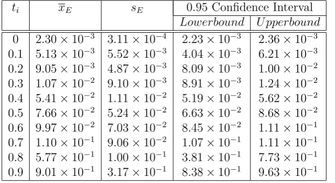
Example 6.2. The following nonlinear Stochastic differential equation is considered [12]

dx(t) = 1 2a

2_n[x(t)]2n−1_dt+a[x(t)]n_{dB(t), t ∈[0 1), (6.2)}

with the exact solution x(t) = x1−₀ n−a(n−1)B(t) 1 1−n_.

The numerical results are shown in Table 2 for n = a = 2. xE is the errors mean and sE is the standard deviation of errors in k iteration.

Table 2: Mean, standard deviation and Confidence Interval for error mean,m= 32, k= 500.

ti xE sE 0.95 Confidence Interval

Lowerbound U pperbound

0 2.30×10−3 3.11×10−4 2.23×10−3 2.36×10−3 0.1 5.13×10−3 5.52×10−3 4.04×10−3 6.21×10−3 0.2 9.05×10−3 4.87×10−3 8.09×10−3 1.00×10−2 0.3 1.07×10−2 9.10×10−3 8.91×10−3 1.24×10−2 0.4 5.41×10−2 1.11×10−2 5.19×10−2 5.62×10−2 0.5 7.66×10−2 5.24×10−2 6.63×10−2 8.68×10−2 0.6 9.97×10−2 7.03×10−2 8.45×10−2 1.11×10−1 0.7 1.10×10−1 9.06×10−2 1.07×10−1 1.11×10−1 0.8 5.77×10−1 1.00×10−1 3.81×10−1 7.73×10−1 0.9 9.01×10−1 3.17×10−1 8.38×10−1 9.63×10−1

7. Conclusion

Acknowledgements

The authors are extending their heartfelt thanks to the reviewers for their valuable suggestions for the improvement of the article.

References

[1] M. Asgari and F. Hosseini Shekarabi, Numerical solution of nonlinear stochastic differential equations using the block pulse operational matrices, Math. Sci. 7 (2013): 47.

[2] M. Asgari, M. Khodabin, K. Maleknejad and E. Hashemizadeh, Numerical solution of nonlinear stochastic Volterra integral equation by stochastic operational matrix based on Bernstein polynomials, Bull. Math. Soc. Sci. Math. Roumanie. 57 (2014) 3–12.

[3] E. Babolian, Z. Masouri and S. Hatamzah-Varmazyar,Numerical solution of nonlinear Volterra-Fredholm integro-differential equations via direct method using triangular functions, Comput. Math. Appl. 58 (2009) 239–247. [4] E. Babolian, H.R. Marzban and M. Salmani,Using triangular orthogonal functions for solving Fredholm integral

equations of the second kind, Applied Mathematics and Computation. 201 (2008) 452–464.

[5] J.C. Cortes, L. Jodar and L. Villafuerte,Mean square numerical solution of random differential equations: Facts and possibilities, Comput. Math. Appl. 53 (2007) 1098–1106.

[6] A. Deb, A. Dasgupta and G. Sarkar, A new set of orthogonal functions and its application to the analysis of dynamic systems, J. Franklin Institute 343 (2006) 1–26.

[7] A. Deb, G. Sarkar and A. Dasgupta, Triangular Orthogonal Functions for the Analysis of Continuous Time Systems, Elsevier, India, 2007.

[8] S. Jankovic and D. Ilic,One linear analytic approximation for stochastic integro-differential eauations, Acta Math. Scientia 30 (2010) 1073–1085.

[9] K. Maleknejad, M. Khodabin and M. Rostami, A numerical method for solving m-dimensional stochastic It-Volterra integral equations by stochastic operational matrix, Comput. Math. Appl. 63 (2012) 133–143.

[10] M. Khodabin, K. Maleknejad, M. Rostami and M. Nouri,Numerical solution of stochastic differential equations by second order Runge-Kutta methods, Math. Comput. Model. 53 (2011) 1910–1920.

[11] F. Klebaner,Introduction to stochastic calculus with applications, Second Edition, Imperial college Press, 2005. [12] P.E. Kloeden, Numerical solution of stochastic differential equations, Applications of Mathematics,

Springer-Verlag, Berlin, 1999.

[13] K. Maleknejad, H. Almasieh and M. Roodaki,Triangular functions method for the solution of nonlinear volterra Fredholm integral equations, Commun Nonlinear Sci Numer Simulat. 15 (2010) 3293–3298.

[14] K. Maleknejad, M. Khodabin and M. Rostami, Numerical solution of stochastic volterra integral equations by stochastic operational matrix based on block puls functions, Math. Comput. Model. 55 (2012) 791–800.

[15] B. Oksendal,Stochastic Differential Equations, An Introduction with Application, Fifth Edition, Springer-Verlag, New York, 1998.