ISSN: 2374-2348 (Print), 2374-2356 (Online) Copyright © The Author(s).All Rights Reserved. Published by American Research Institute for Policy Development DOI: 10.15640/arms.v5n1a2 URL: https://doi.org/10.15640/arms.v5n1a2
Piecewise Linear Economic-Mathematical Models with Regard to Unaccounted
Factors Influence in 3-Dimensional Vector Space
Azad Gabil oglu Aliyev
1Abstract
For the last 15 years in periodic literature there has appeared a series of scientific publications that has laid the foundation of a new scientific direction on creation of piecewise-linear economic-mathematical models at uncertainty conditions in finite dimensional vector space. Representation of economic processes in finite-dimensional vector space, in particular in Euclidean space, at uncertainty conditions in the form of mathematical models in connected with complexity of complete account of such important issues as: spatial in homogeneity of occurring economic processes, incomplete macro, micro and social-political information; time changeability of multifactor economic indices, their duration and their change rate. The above-listed one in mathematical plan reduces the solution of the given problem to creation of very complicated economic-mathematical models of nonlinear type. In this connection, it was established in these works that all possible economic processes considered with regard to uncertainty factor in finite-dimensional vector space should be explicitly determined in spatial-time aspect. Owing only to the stated principle of spatial-time certainty of economic process at uncertainty conditions in finite dimensional vector space it is possible to reveal systematically the dynamics and structure of the occurring process. In addition, imposing a series of softened additional conditions on the occurring economic process, it is possible to classify it in finite-dimensional vector space and also to suggest a new science-based method of multivariate prediction of economic process and its control in finite-dimensional vector space at uncertainty conditions, in particular, with regard to unaccounted factors influence.
Keywords: Finite-dimensional vector space; Unaccounted factors; Unaccounted parameters influence function; Principle of certainty of economic process in fine-dimensional space; Multi alternative forecasting; Principle of spatial-time certainty of economic process at uncertainty conditions in fine-dimensional space; Piecewise-linear economic-mathematical models in view of the factor of uncertainty in finite-dimensional vector space; Piecewise-linear vector-function; 3-Dimensional Vector Space; 2-Component Piecewise-Linear Economic-Mathematical Model in 3-Dimensional Vector Space; Hyperbolic surface.
I. Introduction. Formulation of the problem
In publications [1-5,12] theory of construction of piecewise-linear economic mathematical models with regard to unaccounted factors influence in finite-dimensional vector space was developed. A method for predicting economic process and controlling it at uncertainty conditions, and a way for defining the economic process control function in m-dimensional vector space, were suggested.
In addition to this we should note that no availability of precise definition of the notion “uncertainty” in economic processes, incomplete classification of display of this phenomenon, and also no availability of its precise and clear mathematical representation places the finding of the solution of problems of prediction of economic process and this control to the higher level by its complexity. Many-dimensionality and spatial in homogeneity of the occurring economic process, time changeability of multifactor economic indices and also their change velocity give additional complexity and uncertainty. Another complexity of the problem is connected with reliable construction of such a predicting vector equation in the consequent small volume
V
n1(
x
1,
x
2,...
x
m)
of finite-dimensional vector-space that could sufficiently reflect the state of economic process in the subsequent step. In other words, now by means of the given statistical points (vectors) describing certain economic process in the preceding volume)
,...
,
(
∑
1 2 1 N N m Nx
x
x
V
V
of finite-dimensional vector spaceR
m one can construct a predicting vector equation)
,...
,
(
1 21 m
n
x
x
x
Z
in the subsequent small volume V
n1(
x
1,
x
2,...
x
m)
of finite-dimensional vector space. The goal of our investigation is to formulate the notion of uncertainty for one class of economical processes and also to find mathematical representation of the predicting functionZ
n1(
x
1,
x
2,...
x
m)
for the given class of processes depending on so-called unaccounted factors functions. In connection with what has been said, below we suggest a method for constructing a predicting vector equationZ
n1(
x
1,
x
2,...
x
m)
in the subsequent small volume V
n1(
x
1,
x
2,...
x
m)
of finite-dimensional vector space [1-7, 14].II. Materials and methods:
In these publications, the postulate spatial-time certainty of economic process at uncertainty conditions in finite-dimensional vector space” was suggested, the notion of piecewise-linear homogeneity of the occurring economic process at uncertainty conditions was introduced, and also a so called. The unaccounted parameters influence function
n(
nkn,
n-1,n)
influencing on the preceding volume∑
1 N N n
V
V
of economic process was suggested.
∑
1 22
1 1
1
1
1
(
)
(
)
n-i= i , i-k i i n , n-n n
n
=
z
+A
+
ω
λ
,
α
+
ω
λ
,
α
z
i
(1) Here
ik i ii i k i i
сos
i i , 1 -, 1 -)
,
(
i i k k k i i k i-i k i i k k iсos
a
z
a
a
a
z
z
z
z
z
z
a
z
z
i i-i i , 1 -1 1 1 2 1 1 1 1 -1 -1 1 1 1 -1 -11
-
-)
-(
)
-(
--
1 1 1 -1 1-1
(2)2 1 -1 1 -1 2 -i 1 1
)
(
)
)(
(
)
µ
-µ
(
µ
1 -1 -i 2 -i 1 i i-k i i k i i k i k i-iz
-a
z
-a
z
-a
=
, for
i-1≥
ik-i1-1(3)
n n n n
n n
n(
,
-1, )
сos
-1,
n n k k k n n k n-n k n n k nсos
a
z
a
a
a
z
z
z
z
z
z
a
z
z
n n-n , 1 -1 1 1 2 1 1 1 1 -1 -1 1 1 1 -1 -11
-
-)
-(
)
-(
--
1 1 1 -1 1-1
(3.1))
-(
-)
-(
1 1 1 1 1 1 2 1 1 1 1 1a
z
z
a
z
a
a
A
k k k
2 1 -1 1 -1 2 -n 1 1
)
(
)
)(
(
)
µ
-µ
(
µ
1 -1 -n 2 -n 1 n n-k n n k n n k n k n-nz
-a
z
-a
z
-a
=
, n-1 1 -n ≥ 1 -n k
(5)On this basis, it was suggested the dependence of the n-th piecewise-linear function
z
n on the first piecewise-linear function
z
1 and all spatial type unaccounted parameters influence function
n(
knn,
n-1,n)
influencing on the preceding interval of economic process, in the form Eqs. (1)–(5):
∑
1 22
1 1
1
1
1
(
)
(
)
n-i= i , i-k i i n , n-n n
n
=
z
+A
+
ω
λ
,
α
+
ω
λ
,
α
z
i
(6) Where
ik i ii i k i i
сos
i i , 1 -, 1 -)
,
(
i i k k k i i k i-i k i i k k iсos
a
z
a
a
a
z
z
z
z
z
z
a
z
z
i i-i i , 1 -1 1 1 2 1 1 1 1 -1 -1 1 1 1 -1 -11
-
-)
-(
)
-(
--
1 1 1 -1 1-1
(7)are unaccounted parameters influence functions influencing on the preceding
V
1, V
2,..V
i small volumes of economic process; 2 1 1 1 1 2 1 -1-)
z
-(
)
z
-)(
z
-(
)
-(
1 1 2 1 - i-i k i-i k i-i k i-i k i i ia
a
a
, for 11
1 µ
µ k
i-≥
i- (8)
are arbitrary parameters referred to the i-th piecewise-linear straight line. And the parameters
i are connected with the parameter
i-1 referred to the (i-1)-th piecewise-linear straight line, in the form Eq. (8);)
-(
-)
-(
1 1 1 1 1 1 2 1 1 1 1 1a
z
z
a
z
a
a
A
k k k
(9)is a constant quantity;
n n n
n n n
n(
,
-1, )
сos
-1,
n n k k k n n k n-n k n n k nсos
a
z
a
a
a
z
z
z
z
z
z
a
z
z
n n-n , 1 -1 1 1 2 1 1 1 1 -1 -1 1 1 1 -1 -11
-
-)
-(
)
-(
--
1 1 1 -1 1-1
(10)is the expression of the unaccounted parameters influence function that influences on subsequent small volume
V
Nof finite-dimensional vector space. And the parameter
n referred to the n- piecewise-linear straight line is of theform: 2 1 -1 1 -1 2 -n 1 1
)
(
)
)(
(
)
µ
-µ
(
µ
1 -1 -n 2 -n 1 n n-k n n k n n k n k n-nz
-a
z
-a
z
-a
=
, n-1
1 -n ≥ 1 -n k
(11)After that, in publications [6-11,13-15] a solution was found of solve a problem on prediction of economic process and its control at uncertainty conditions in finite-dimensional vector space. It became clear, that the unaccounted parameters influence functions
n(
n,
n-1,n)
are integral characteristics of influencing external factors occurring in environment that are not a priori situated in functional chain of sequence of the structured model but render very strong functional influence both on the function and on the results of prediction quantities Eq. (6). It is impossible to fix such a cause by statistical means. This means that the investigated this or other economic process in finite dimensional vector space directly or obliquely is connected with many dimensionality and spatial inhomogenlity of the occurring economic process, with time changeability of multifactor economic indices, vector and their change velocity. This in its turn is connected with the fact that the used statistical data of economic process in finite-dimensional vector space are of inhomogeneous in coordinates and time unstationary events character.We assume the given unaccounted factors functions
n(
n,
n-1,n)
hold on all the preceding interval of finite-dimensional vector space, the uncertainty character of this class of economic process. In such a statement, the problem on prediction of economic event on the subsequent small volume V
N1 of finite-dimensional vector space will be directly connected in the first turn with the enumerated invisible external facts fixed on the earlier stages and their combinations, i.e., the functions
n(
n,
n-1,n)
that earlier hold in the preceding small volumesN
V
V
V
1
,
2,
...
of finite-dimensional vector space. Therefore, by studying the problem on prediction of economic process on subsequent small volume V
N1 it is necessary to be ready to possible influence of such factors. In connection with such a statement of the problem, let’s investigate behavior of economic process in subsequent small volume V
N1 finite-dimensional vector space under the action of the desired unaccounted parameters function)
,
(
n n-1,nn
that was earlier fixed by us in preceding small volumes V
n of finite-dimensional vector space, i.e.,)
,
(
2 1,22
,
3(
3,
2,3)
, ….,
N(
N,
N-1,N)
. In connection with what has been said, the problem on prediction of economic process and its control in finite-dimensional vector space may be solved by means of the introduced unaccounted parameters influence function
n(
n,
n-1,n) in the following way. Construct the (N+1)-thevector equation of piecewise-linear straight line 1
µ
N 1(
2 N)
N N
N
k N k
N
=
z
+
a
z
z
depending on the vector equation of
the first piecewise-linear straight line
z
1 and the desired unaccounted parameter influence function
(
,
-1,)
That we have seen in one of the preceding small volumes V
1,
V
2,
...
V
N of finite-dimensional vector space. For that in Eqs. (6)–(11) we change the index n by (N1) and get:
1
1
(
)
1(
1 1)
2
1 1
1
∑
N N N,NN
i=
i , i-k i i
N
=
z
+A
+
ω
λ
,
α
ω
λ
,
α
z
i
(12)
Here
ik i ii i k i
i
сos
i i
, 1 -,
1 -
)
,
(
i i k
k
k i i
k i-i k i i k
k
сos
a
z
a
a
a
z
z
z
z
z
z
a
z
z
i i-i
i i
, 1 -1
1 1 2
1 1 1
1 -1 -1
1 1 1 -1
-1
1
-
-)
-(
)
-(
--
11 1
-1 1
-1
(13)2 1 -1
1 -1 2 1
1
)
(
)
)(
(
)
µ
-µ
(
µ
1
-1 -i 2
1
i
i-k i i
k i i k i-i k i-i
z
-a
z
-a
z
-a
=
, 1
1 1
i-k i-≥ i-
(14))
-(
-)
-(
1 1 1
1 1 1 2 1
1 1
1 1
a
z
z
a
z
a
a
A
kk k
(15)
1
(
N 1,
N,N 1)
N 1 N,N 1N
сos
1 , N 1
1 1 2
1 1 1
N 1
2 N
1
1
-
-)
-(
)
-(
-1 1 N
1 1
N k
k
k N
k N N k N
k
сos
a
z
a
a
a
z
z
z
z
z
z
a
z
z
N NN
(16)
2 2
2 1 1 1
)
(
)
)(
(
)
µ
-µ
(
µ
1
N N
N-N
k N N
k N N k N-N k N N N
z
-a
z
-a
z
-a
=
,
N k N N≥
(17)For the behavior of economic process on the subsequent small volume
V
N1 of finite-dimensional vectorspace to be as in one of the desired preceding ones in small volume ΔVβ it is necessary that the vector equations of
piecewise-linear straight lines zN1 and
z
β to be situated in one of the planes of these vectors and to be parallel to one another, i.e.β
1
N
С
z
z
(18)
In connection with what has been said, to
V
N1 finite-dimensional space there should be chosen such a vector-point 2 N
a
that the piecewise-linear straight lines 1 ( 2 kN)N N
N a z
z
and z (a z )
1
β
k 1
β
1
β β
could be situated in the same plane of these vectors and at the same time be parallel to each other (Fig. 1).
Fig. 1. The scheme of construction of prediction function of economic process
Z
N1(
)
at uncertainty conditions in finite-dimensional vector spaceR
m. Prediction functionZ
N1(
)
will lie in the same plane with one of the desired preceding
-the piecewise-linear straight line and will be parallel to it.In other words, they should satisfy the following parallelism condition:
)
( 2 kN
N N z
a = С(a zkβ1)
1
β
1
β
(19)
Here
m M
m
m N
N a i
a
1 , 2
2 ,
M
1 m
m m 1,
β
1
β a i
a ,
M
m
m k
m N k
N z i
z N N
1 ,
,
M
1 m
m k
m 1,
β
k 1
β z i
z β1 β1
1 β k 1,1 β 1,1 β 1 , 1 , 2 z a
kN N N z a = 1 β k 1,2 β 1,2 β 2 , 2 , 2 z a
kN N N z a =.….= 1 β N k M 1, β M 1, β k M N, M 2, N z a z a (20) It is easy to define from system Eq. (20) the coefficients of the vector
a
N2:)
(
z
a
z
a
z
a
k 2,1 ,11,1 β 1,1 β k 1,2 β 1,2 β k N,2 2,2
N β1
1
β
N kN
N N
z
a
) z (a z a z a z a N 1 β N k N,1 2,1 N 1,1 β 1,1 β k 1,3 β 1,3 β k N,3 2,3 N )
z
(a
z
a
z
a
z
a
N 1 β 1 β N k 1 M N, 1 M 2, N k 1 M 1, β 1 M 1, β k M 1, β M 1, β k M N, M 2,N
(21)In this case, the vector
a
N2
will have the following final form:
2
N
a
=a
N2,1i
1
a
N2,2i
2
a
N2,3i
3
...
a
N2,Mi
M (22)As the coordinates of the point (of the vector)
a
N2
now are determined by means of the piecewise-linear
vector kβ1
1
β
1
β
β a z
z taken from one of the preceding stage of economic process, it is appropriate to denote them in the form
a
N2(
)
[8-13]. This will show that the coordinates of the point
a
N2
(3) were determined by means of piecewise-linear straight line zβ
. In this case it is appropriate to represent Eq. (22) in the following compact form:
M m m m NN a i
a
1 , 2
2( ) ( )
(23)Now, in the system of Eqs. (12)–(17), instead of the vector
a
N1
we substitute the value of the vector
a
N2(
)
, and also instead of
N1(
N1,
N,N1)
introduce the denotation of the so-called predicting influence function with regard to unaccounted parameters
N1(
N1,
N,N1)
. In this case the prediction function of the economic process)
(
1
N
Z
with regard to influence of prediction function of unaccounted parameters N1(λN1,αN,N1) will takethe following form:
(
)
1
1
(
)
1(
1 1)
2
1 1
1
∑
N N N,NN i= i , i-k i i
N
=
z
+A
+
ω
λ
,
α
λ
,
α
Z
i (24)Here
ki i ii i k i i
сos
i i , 1 -, 1 -)
,
(
i i k k k i i k i-i k i i k kсos
a
z
a
a
a
z
z
z
z
z
z
a
z
z
i i-i i i , 1 -1 1 1 2 1 1 1 1 -1 -1 1 1 1 -1 -11
-
-)
-(
)
-(
--
1 1 1 -1 1-1
(25)2 1 -1 1 -1 2 1 1
)
(
)
)(
(
)
µ
-µ
(
µ
1 -1 -i 2 1 i i-k i i k i i k i-i k i-iz
-a
z
-a
z
-a
=
, 1
1 1 i-k i-≥ i-
(26))
-(
-)
-(
1 1 1 1 1 1 2 1 1 1 1 1a
z
z
a
z
a
a
A
k k k
(27)1 , 1 1
, 1
1
(
,
)
N
N
N N
Nсos
N N (28)1
N
1 1 1 2
1 1 1
N 1
2 N
1
1
-
-)
-(
)
-(
-)
(
-1 1 N
1 1
a
z
a
a
a
z
z
z
z
z
z
a
z
z
k k
k N
k N N
k N k
N N
N
(29)
2 2
2 1 1 1
)
)
(
(
)
)
(
)(
(
)
µ
-µ
(
µ
1
N N
N-N
k N N
k N N
k N-N k N N N
z
-a
z
-a
z
-a
=
, N
k N N≥
(30)Here the vector
a
N2(
)
is determined by Eq. (23).
Note the following points. It is seen from Eq. (11) that for kN N N
the value of the parameter
N1
0
. By this fact from Eq. (28) it will follow that the value of the predicting function of influence of unaccounted parameters) ,
( 1 , 1
1
N
N
N N will equal:) ,
( 1 , 1
1
N
N
N N =0 for
N1
0
N1(
N1,
N,N1) 0 for
N1
0
(31)This will mean that the initial point from which the (N+1)-th vector equation of the prediction function of economic process ZN1(
)
will enanimate, will coincide with the final point of the n-th vector equation of piecewise-linear straight line
z
N
and equal:
∑
2
1 1
1
1
1
(
)
N
i=
i , i-k i i N
=
z
+A
ω
λ
,
α
Z
i , for0
1
N
(32)For any other values of the parameter
N1
0
the points of the (N 1)-th vector equation will be determined by Eq. (24). It is seen from Eq. (28) that
N1 0 and N1(
N10;
N,N1)0 will follow сos
N,N1 0 and0
1
N
. This will correspond to the case when the influence of external unaccounted factors on subsequent small volume V
N1 are as in the preceding small volume V
N of finite-dimensional vector space. In this case it suffices to continue the preceding vector equationz
N to the desired point kNN N
N
1 *1 of subsequent small volume of finite-dimensional vector space.The value of the vector function ( ) ( ; , 1, )
* 1 *
1
1 N N N N N N
N z
Z
at the point
N1
*N1 will be one of the desired prediction values of economic process in subsequent small volume V
N1. In this case, the value of thecontrolled parameter of unaccounted factors will be equal to zero, i.e.,
0
)
0
;
0
сos
;
0
;
0
(
1 1 N,N 1 , 11
N
N
N
N NFor any other value of the parameter
N1, taken on the interval 0
N1
N*1 and сos
N,N10, the corresponding prediction function of unaccounted parameters will differ from zero, i.e., N1(
N1,
N,N1)0.Thus, choosing by desire the numerical values of unaccounted parameters function ωβ(µN1;λβ,αβ1,β)
)
α
,
(
λ
Ω
N1 *N1 N,N1 corresponding to preceding small volumes V
1,
V
2,
...
V
N and influencing by them beginning with the point
N1
0
to the desired point
*N1, we get numerical values of predicting economic event)
,
;
(
* 1 * 1 , 11
N N N N
N
Fig. 2. The graph of prediction of process and its control at uncertainty conditions in finite-dimensional vector space. It is represented in the form of hypersonic surface whose points, of directrix will form the line of economic process prediction. Taking into account the fact that by desire we can choose the predicting influence function of unaccounted parameters
*N1(
N*1;
N1,
N,N1)
, then this function will represent a predicting control function of unaccounted factors, and its appropriate function(
;
1,
, 1)
* 1 , *
1
N N N N N N
Z
will be a control aim function of economic event in finite-dimensional vector space. Speaking about unaccounted parameters prediction function) ,
;
( 1 1 , 1
1
N
N
N
N Nwe should understand their preliminarily calculated values in previous small volumes
V
1,
V
2,
...
V
N offinite-dimensional vector space. Therefore, in Eq. (24) we used calculated ready values of the function
) ,
;
( 1 1 , 1
1
N
N
N
N N .Thus, influencing by the unaccounted parameters influence functions of the form) ,
;
( 1 1 , 1
1
N
N
N
N N or by their combinations from the end of the vector equation of piecewise-linear straight line ( ; , N-1,N)k N k N k N
N N N
z
situated on the boundary of the small volume
Z
N1(
)
ZN1(N1;N1,N,N1)
there will originate the vectors
V
N and V
N1, lying on the subsequent small volume V
N1.These vectors willrepresent the generators of hyperbolic surface of finite-dimensional vector space. The values of this series vector-functions for small values of the parameter
N1
*N1, i.e., ( * ; 1, , 1)1
1
N N N N
N
Z will represent the points directrix of hyperconic surface of finite-dimensional vector space (Fig. 2). The series of the values of the points of directrix hyperconic surface will create a domain of change of predictable values of the function of
)
,
;
(
* 1 1 , 1*
1
N N N N
N
Z
in the further step in the small volume V
N1.This predictable function will haveminimum and maximum of its values
[
Z
*N1(
N*1;
N1,
N,N1)]
min and[
Z
N*1(
N*1;
N1,
N,N1)]
maх. Thus, the found domain of change of predictable function of economic process in the form ( ; 1, , 1)* 1
1
N N N N
N
Z , or in
other words, the points of directrix of hyperbolic surface will represent the domain of economic process control in finite-dimensional vector-space.
In this article we give a number of practically important piecewise-linear economic-mathematical models with regard to unaccounted parameters influence factor in their-dimensional vector space. And by means of two- and three-component piecewise-linear models suggest an appropriate method of multivariant prediction of economic process in subsequent stages and its control then at uncertainty conditions in 3-dimensional vector space [6-11,13-15].
Given a statistical table describing some economic process in the form of the points (vector) set
{
a
n}
of 3-dimensional vector spaceR
3. Here the numbersa
ni are the coordinates of the vectora
n
(an1,an2,an3, ……ani). With
the help of the points (vectors)
a
n represent the set of statistical points in the vector form in the form of 2-component piecewise-linear function [1–6]:
)
-(
2 11 1
1
a
a
a
z
(33))
-(
3 22 2
2
a
a
a
z
(34)Here
z
1
z
1(
z
11,
z
12,
z
13)
andz
2
z
2(
z
21,
z
22,
z
23)
are the equations of the first and second piecewise-linear straight lines on 3-dimensional vector space; the vectorsa
1(
a
11,
a
12,
a
13)
,a
2
a
2(
a
21,
a
22,
a
23)
and)
,
,
(
31 32 333
3
a
a
a
a
a
are the given points (vectors) in 3-dimensional space;
1≥
0
and
2≥
0
are arbitrary parameters of the first and second piecewise-linear straight lines. And it holds the equality
1
1
1
and1
2 2
;
1,2 is the angle between the piecewise-linear straight lines;k
1 is the intersection point between the first and second straight lines (Fig. 3). Note that in the general case, the intersection point of these straight lines may also not coincide with the pointa
2. Therefore, according to the conjugation condition 1 12 1
k k
z
z
, we denote the intersection point between the first and second piecewise-linear straight lines in 3-dimensional vector space by1 1
k
z
(Fig. 3). Allowing for this fact, we write the equation of the second piecewise-linear straight line in the form Eq.
(35): 1 ( - 1)
1 3 2 1 2
k k
z a z
z
(35) where the valuez
1k1 is the value of the point (vector) of the first piecewise-linear straight line at thek
1-the intersection point and equals:Fig. 3. Construction of 2-component piecewise-linear economic-mathematical model
In 3-dimensional vector space
R
3.)
-(
2 11 1 1
1
1
a
a
a
z
k k
In particular case, 1 2 1
a
z
k
for 11
1
k
. In this case, the intersection point 1 1k
z
coincides with the pointa
2. Now, according to Eqs. (1)–(11) of, the vector equation for the points of the second piecewise-linear straight line depending on the vector function of the first piecewise-linear straight linez
1 and introduced unaccounted parameters influence spatial function
2(
2,
1,2) in 3-dimensional vector space is written in the form (Fig. 3) [7–9]:)]}
(
1
[
1
{
2 2 1,21
2
=
z
+A
+
ω
λ
,
α
z
(37) Here ) -( -) -( 1 1 1 1 1 1 2 1 1 1 1 1 a z z a z a a A k k k
(38)
1 1 1 2 1 1 1 1 1 1 1 3 1 1 1 1 2 2
-)
-(
)
-(
--
1 1 1 1 1 1a
z
a
a
a
z
z
z
z
z
z
a
z
z
k k k k kk
(39)2 , 1 2 2 , 1 2
2(
,
)
сos (40)2 1 3 1 2 1 3 1 1 2
)
(
)
)(
(
)
µ
-µ
(
µ
1 1 1 k k kz
-a
a
-a
z
-a
=
, for 1
1
≥
1
k
(41)Eq. (41) is the mathematical relation between arbitrary parameters
2 and
1. For the second piecewise-linear straight line, representing a straight line restricted with one end, condition Eq. (41) will hold for all 11 ≥ 1 k
.Furthermore, for the second intersection point
k
2, i.e., for 2 2 2k
, the appropriate value of the parameter
1 will be determined as follows:2 1 1 1 2 2 1 2 1 3 2 1 3 1 1
)
)(
(
)
(
k k k k ka
a
z
a
z
a
(42)The value of сos
1,2 between the first and second piecewise-linear straight lines is determined by means of the scalarproduct of 2 vectors of the form (Fig. 3):
1 1 1 1 1 2 1 1 1 2 1 1 2 , 1
)
)(
(
k k k kz
z
z
z
z
z
z
z
C
A
B
A
C
A
B
A
сos
(43)By calculating the values of сos
1,2 we can use any values of arbitrary parameters
1 and
2. Thus, in 3-dimensional vector space, determining the points (vectors):∑
3 1 1 1
m m mi
a
a
,∑
3 1 2 2
m m mi
a
a
,∑
3 1 3 3
m m mi
a
a
m
m m m
k m
m m
k m
k
z
i
a
a
a
i
z
31 1 1 2 1
3
11
11
∑
1[
1(
-
)]
(44)Eq. (37) will represent an equation for the second vector straight line
z
2=
z
2(µ
1,
ω
2)
depending on the unaccounted parameter influence function
2(
2,
1,2) and arbitrary parameter 11
1
≥
k
. Represent the vector equation for the second piecewise-linear straight line Eq. (37) in the coordinate form. For that take into account that in 3-dimensional space the vectors of the first and second piecewise-linear straight lines in the coordinate form are represented in the form:∑
3 1 1 1
m m mi
z
z
and
∑
In this case, the coordinates of the vector
z
2 Eq. (37), i.e., z2m will be expressed by the coordinates of the first piecewise-linear vector z1m, spatial vector
2 and the unaccounted parameter influence function
2(
2,
1,2), inthe form:
1m 2 , 1 2 2
2
=
{
1
+A
[
1
ω
(
λ
,
α
)]}z
z
m
, for m1,2,3 (46)Here the coordinate notation of the coefficients A,
2 and
2(
2,
1,2), by Eqs. (38)–(41), will be of the form:∑
∑
3
1
1 2 1 1 1 2
3
1
2 1 2
1 1
)] -( )[
-(
) -( )
-( 1
i
i i i
i i
i
i i k
a a a
a a
a a A
(47)∑
∑
3
1
2 1 2
2 3
1
1 2 1 1 3
1 1
2 2
)
-(
}
)]
-(
[
-{
-1
i
i i i
i i k i i
k
a
a
a
a
a
a
(48)2 , 1 2 2 , 1 2
2(
,
)
сos (49)∑
∑
3
1
2 1 2 1 1 3
1 2 1 1 3 3
1
1 2 k
1 1 2
)] -( -[
)] -( -[ ) -( ) µ -(µ
1 1 1
i
i i k i i
i i k i i i
i i
a a a
a
a a a
a a a
, for 11 1
k
(50)) -( )] -( -[
)] -( -[ ) -(
1 2 1
1 2
1 1 3
1
2 1 2 1 1 3
1 2 1 1 3 3
1
1 2
2
∑
∑
k k
i
i i k i i
i i k i i i
i i k
a a a
a
a a a
a a a
(51)
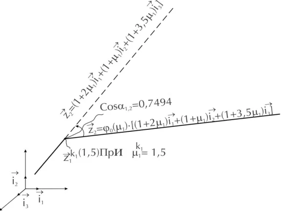
Now, for the case economic process represented in the form of 2-component piecewise-linear economic-mathematical model, investigate the prediction and control of such a process on the subsequent
V
3(
х
1,
х
2,
х
3)
small volume of 3-dimensional vector space with regard to unaccounted parameter influence function
2(
2,
1,2).And the value of the unaccounted parameter
2(
2,
1,2) function is assumed to be known [6-11,13-15]. A methodfor constructing a predicting vector function of economic process
Z
N1(
)
with regard to the introduced unaccounted parameters influence predicting function N1(
N1,
N,N1) in m-dimensional vector space, represented by Eqs. (24)–(30) was developed above. Apply this method to the case of the given 2-component piecewise-linear economic model 3-dimensional vector space. It will be of the form:)]}
,
(
)
,
(
1
[
1
{
)
1
(
1 2 2 1,2 3 3 2,33
2
z
A
kZ
(52)Where
2 1,22 , 1 2 2
2 2