,PSURYLQJ3UHGLFWLRQV8VLQJ/LQHDU&RPELQDWLRQ
RI0XOWLSOH([WUHPH/HDUQLQJ0DFKLQHV
3HGUR-*DUFtD/DHQFLQD
Centro Universitario de la Defensa de San Javier, (University Centre of Defence at the Spanish Air Force Academy)
Ministerio de Defensa-Universidad Politécnica de Cartagena
http://dx.doi.org/10.5755/j01.itc.42.1.1667
$EVWUDFW. This work presents several effective approaches for linear combination of multiple artificial neural networks based on the extreme learning machine (ELM) algorithm. Given a learning task, a large set of neural networks are firstly trained by ELM. Then, these trained machines are efficiently ranked and the useless models are effectively discarded in order to provide an ensemble system with better generalization performance. The ensemble system is constructed using an automatic and fast forward model selection by minimizing the leave-one-out error, without user intervention. Experiments on an artificial regression dataset and three real-world engineering problems are discussed. According to the obtained results, the weighted linear combination of ELMs improves predictions by exploiting model diversity in the ensemble system with fast learning speed.
.H\ZRUGV: Artificial neural network (ANN); Extreme learning machine (ELM); Linear combination; Ensembles; Regression.
,QWURGXFWLRQ
Artificial neural networks (ANN) have been successfully applied to many engineering and science fields [1]. Thus, they have been used to solve problems in industrial applications as control processes, fault detection and quality evaluation; in security applications based on biometric recognition; in medical applications as diagnosis, detection and evaluation of medical phenomena; in financial applications as stock market prediction, credit worthiness, credit rating, bankrupt prediction, and prices forecasts; and finally, in many others fields of the science as biological systems analysis, botanical recognition, recipes and chemical formulation optimization, and ecosystem evaluation.
ANN modelling often entails the construction of multiple networks with different architectures, learning procedures and training parameters in order to obtain an accurate model. Typically, one of the trained ANNs is usually chosen as the ‘best’ model and the remaining networks are discarded. Instead of using an individual network, it is widely known that combining the estimates of multiple models can improve the performance of the best network in the ensemble [2]–[5].
In general, a neural network ensemble is constructed in two main steps: training a number of
appropiate techniques for robust and fast design of ELM networks [10].
With respect to the second stage of the ensemble construction, the output of the ensemble system is computed by combining the outputs of each model, being simple averaging or weighted averaging the most prevailing approaches for regression tasks. At this point, it is important to remark that, in practice, most ensemble approaches use all of those trained networks to design the ensemble system and assign weight values according to its contribution to the ensemble. Some recent works have proposed adaptive ensembling approaches for neural networks [4], but their major drawbacks are that they are sensitive to random subsampling of validation sets and, also, they require to tune a threshold parameter for performing model selection. In this work, the most useful/accurate models for the ensemble are fast automatically chosen and it is done without user intervention. Particularly, after the different networks have been trained, their outputs are ranked according to the multiresponse sparse regression (MRSR) method, which determines the contribution of each individual model in the ensemble to the global prediction of the target variable. Once the candidate networks are ranked, the better models are chosen following an incremental forward selection methodolody by fast minimization of the leave-one-out (LOO) error, which is exactly measured with the predicted residual sums of squares (PRESS) statistic. As it is described in next sections, the model selection is not sensitive to random subsampling of validations sets (all samples are used for training and validation) and there is not any tuneable parameter for perform model selection.
Finally, it is widely known that the success of an ensemble system relies upon the diversity among the individual models, i.e. hypotheses disagree with each other in many of the individual model predictions. Diversity is a key aspect since it may determine whether the ensemble will perform better than its individual components. In this work, model diversity is exploited by varying the input layer of the individual models. Three different scenarios are evaluated: the original feature input space, the resulting reduced feature subset by forward selection and random input subspaces.
The rest of this paper is organized as follows: Section 2 gives an overview of the ELM algorithm for training SLFNs and some of its extensions for automatic design of the neural architecture. The ensemble approaches for ELM networks are described in Section 3 and Section 4 gives experimental results on four well-known regression problems. Finally, the main conclusions and future works are reported in Section 5.
(/0DOJRULWKPIRUWUDLQLQJ6/)1V
Consider a dataset defined by ܰsamples (ݔ,ݐ), where ݔ=ൣݔଵ,ݔଶ, … ,ݔ൧
்
א Թ is the j-th input
vector and ݐ א Թis its corresponding target value. This dataset is learned using a SLFN with M hidden neurons and activation function ݂(·), which is mathematically modeled as
= ݒ݂൫ܟ்ܠ+ܾ൯ ெ
ୀଵ
= ݒ݄
ெ
ୀଵ
,݆= 1, … ,ܰ; (1)
where ݓ= [ݓଵ,ݓଶ, … ,ݓ]் is the weight vector
connecting the i-th hidden neuron and the input units,
ݒis the weight connecting the i-th hidden neuron and
the output unit, and ܾis the threshold of the i-th hidden neuron. Besides, ݄is the i-th hidden output for ݔ. Note that the network output unit is linear.
Figure 1 shows a scheme of a SLFN architecture with single hidden layer of neurons. One of the most popular activaction function is the sigmoid and, in this case, the SLFN is widely known as multi-layer perceptron (MLP). The learning objective is that
ൎ ݐ with a good generalization capability.
)LJXUHStandard neural architecture of a SLFN with
single hidden layer of ܯneurons. The input layer is composed of ݊and the output layer has one unit
The standard ELM method is based on the concept that if input weights wand biases ܾare randomly assigned, then a SLFN can be considered as a linear system and the output weight vector, v, can be analytically determined through simple generalized inverse operation of the hidden layer output matrices [6]–[8]. For fixed wand b, thetraining of a SLFN is simply equivalent to find a leastsquares solution, vො, for the linear system ۶ܞ=ܜ, where
۶=
݂(ܟଵ்ܠଵ+ܾଵ) … ݂(ܟெ்ܠଵ+ܾெ)
ڭ … ڭ
݂(ܟଵ்ܠே+ܾଵ) ڮ ݂(ܟெ்ܠே+ܾெ)
ே×ெ
(2)
From [7], [8], the solution is analytically given by
ܞො=થறܜ, where થறis the Moore-Penrose generalized
calculate થற for faster computations and numerical
stability. ELM is a batch learning approach much simpler and faster than traditional learning algorithms for SLFN. Without iteratively tuning parameters as in standard training procedures, the learning speed of ELM can be thousands of times faster than the gradient based learning algorithms. Given enough hidden neurons, the performance of this simple learning algorithm is comparable to traditional gradient based algorithms in terms of predictive accuracy results.
A. Automatic design of neural networks based on ELM
As it have been already mentioned, the ELM algorithm provides an analytical training procedure for a SLFN with a fixed architecture (i.e., a predefined hidden layer size, ܯ) and randomly assigned hidden parameters. However, the optimal network size is usually unknown and tedious experimentation becomes necessary to find a good network. It means that an exhaustive search of ܯis done by means of a cross-validation procedure [1], which may imply an excesive computational cost in large datasets. Although the advantages of the ELM algorithm have been proved in many scientific areas, it has been found that the obtained networks tend to require more hidden nodes than traditional training methods because the random assignment of parameters may introduce inappropriate values for them. Several growing [12]–[14] and pruning [10], [15], [16] improvements for the ELM algorithm have been proposed in order to obtain a more compact network and to avoid an extensive search of the optimal hidden layer size. It has been shown that, in general, the growing techniques are more sentitive to the random weight initialization than prunning procedures and, then, they can be trapped in a sub-optimal solution. From the different pruning approaches, the optimally pruned ELM (OP-ELM) methodology stands out as a robust and fast technique for automatic design of ELM networks [10].
The OP-ELM method [10] improves the standard ELM algorithm by pruning inappropiate hidden nodes using an exact and efficient ranking criterion, which is based on the multiresponse sparse regression (MRSR) algorithm and the prediction sum of squares (PRESS) statistic. As it is shown in [10], OP-ELM provides extremely fast accurate models and achieves roughly the same level of accuracy as that of other well known machine learning methods, such as support vector machines (SVM) or gaussian processes (GP). In what follows, the three main stages of the OPELM method are outlined.
1. Random initialization of a large SLFN. This first step is performed using the standard ELM algorithm for a large enough number of neurons, ܯ. From a practical point of view, it is advised to set ܯclearly above the number of input features: ܯ ب ݊ . For sigmoid functions, the weights are drawn randomly
from an uniform distribution in an interval that covers the input data range (previously normalized to zero mean and unit variance) [10].
2. Ranking of hidden units. In a second stage, the MRSR algorithm is applied in order to rank the hidden neurons according to their accuracy. This method is based on a regularization approach inspired by the LASSO methodology [17], which minimizes the residual sum of squares while bounding the L1-norm of the weight vector by a specified value. MRSR is in essence an extension of the wellknown least angle regression (LARS) algorithm and, hence, it is a variable ranking technique [18], rather than a selection one. It must be outlined that the obtained ranking by MRSR is exact for linear problems [17]. Since the output of an ELM network is linear with respect to the randomly initialized hidden units, the obtained ranking of neurons by MRSR is exact [10]. More details of the MRSR method can be found in [17].
3. Selection of hidden units. Once the ranking of the hidden neurons has been obtained and
۶ is consequently ordered, the best ܯכ
hidden units for the ELM model are chosen using the LOO error, which can be exactly calculated for linear models by using the PRESS statistic [19]. Consider that ܞො()is the
least-squares error solution when the j-th sample (j-th row of۶) is omitted, i.e.,
ܞො()=۶(ற)ܜ(), (3)
where ۶() and ܜ(ܒ) are, respectively, ۶
without its j-th row and t without its j-th component vector.
Then, the LOO error is given by
אோாௌௌ= 1
ܰฮܐܞො()െ ܜ()ฮ
ଶ ே
ୀଵ
, (4)
where h is the j-th row of ۶. To select a
model by using the LOO error as criterion, the אோாௌௌfor each model is computed and
the model with a minimal אோாௌௌis chosen.
Directly using the previous formula the computation of _PRESS would be extremely inefficient and computationally prohibitive since the model has been computed as many times as the number of samples. However, it is well-known that there is a non-iterative and exact formula giving the PRESS statistic as:
אோாௌௌ= 1
ܰԡȞ(ધ െ ય)
ିଵ(ય െ ધ)ԡ ࣠ ଶ , (5)
with ۾ = ۶۶ற,۷is the identity matrix and
denotes the matrix Frobenius norm of ۯ. A proof of formula (5) is given in [20].
For OP-ELM networks, the PRESS statistic is iteratively computed by adding a hidden node (which are previously ranked in ۶) to the model. The model with ܯכ hidden
neurons obtains the lowest PRESS statistic and this model is considered optimal, i.e.,
אܴܲܧܵܵெ כ
< אܴܲܧܵܵ ,݇ א(1, 2, … ,ܯ). (6)
On the contrary to the standard ELM algorithm, OPELM does not need to divide learning set into training and validation subsets because it directly determines the optimal hidden layer size by computing the LOO error with the PRESS statistic. Therefore, OP-ELM is faster than the standard ELMalgorithm and it uses more trainingsamples. Note that OP-ELM provides a SLFN with different hidden layer size for each input weight initialization.
/LQHDUFRPELQDWLRQRI(/0V
It is widely known that the performance of a SLFN can be improved by combining several solutions to the same task, i.e., by combining the outputs of different individual ELMs. Rather than generating a population of ܮ modelsand using a single ’best’ model in isolation, a combinationof these ܮ networks would exploit, rather than ignore, the information contained in the redundant models. Such combination of models is sometimes called committees or ensembles. Two main issues arise when considering the ensemble approach: first, the creation of ܮ models to be
combined in an ensemble; and second, the method by which the outputs of the members are combined [2]. In the first step, note that when the trained networks which all generalised identically are combined in a ensemble system, there will be no improvement in performance between the outputs from the individual models and the ensemble of them. In order to the models generalize differently, they must each have their initial conditions varied prior to creation (for example, by varying initialweights or topology) or different training data set (forexample, by varying training sets or input features). Withrespect to the second issue, the simplest way to constructa commitee is to average the predictions of a set ofܮindividual ELM models (with the same number of hidden neurons and different weight initializations) [21], but other combination schemes are also possible.
Liu and Wang presented an ensemble ELM method which uses a cross-validation scheme in order to increase the diversity between the individual models [22]. This procedure trains ܭ ELM networks on different R pairsof data sets which are generated by cross-validation. Whereas, [22] uses the same hidden layer size for all ܴ × ܭ ELMs and it does not perform a selection of appropiate candidate networks for the ensemble. In order to discard inaccurate individual models, Chen et al. [23] measure the
diversity between individual models (with a predefined hidden layer size) and the ensemble output using the Pearson correlation coefficient and then computes its product with the mean square error (MSE) of each model. In particular, it discards a network from the ensemble if its corresponding product is greater than the mean value of all product results [23], which means that discarded models have large MSE and small diversity. Heeswijk et al. [24] introduce an adaptive ensemble of random ELM networks for time series prediction where its ensemble weights (with positivity constraints) are iteratively updated according to a predefined learning rate. This procedure can be very expensive in computational terms. For solving this inconvenient, Heeswijk et al. [25] implement the ELM algorithm using GP (Graphics Processing) computing (instead of standard CPU implementation) in order to reduce the training time. Nevertheless, this technique is quite sensitive on the correct choice of the validation set and its results vary if the analysis is repeated with different random splits.
This section presents robust and fast approaches for ensembling ELMs by exploiting model diversity. In particular, consider a linear combination scheme of
ܮELM networks,
ݕ= ݄
ୀଵ
, (7)
where ݕis the ensemble output and ߣis ݈-th ensemble
weight. Thus, given the ܰinput vectors, the following problem must be solved:
ݕ= ߣߧ
ୀଵ
ൎ ݐ ,݆= 1, … ,ܰ; (8)
where ojl is the prediction of the ݈-th model given ݔ݆
and ߣis the ensemble weight vector connecting the ݈ -th model and -the output units. The ensemble weights can be obtained by the least-squares solution of (8):
ߣ=ભறલ , where ભற denotes the Moore-Penrose
generalized inverse of the network output matrix ભ,
whose ݈-th column is the l-th network’s ouput vector for the ܰ input vectors. Here, this ensembling procedure is known as least-squares combination of ELMs (LSC-ELM).
Instead of using all the ܮmodels, the ܮכnetworks
(with ܮכ ܮ) whose linear combination provides
better generalization capability are chosen. From the basis of the OP-ELM methodology, a direct and exact linear combination of the ܮכ chosen networks is
different random subsets of features. Each candidate network for the ensemble system is trained using the OP-ELM algorithm, as in [24]. On the contrary to other ensembling methods, this procedure has more diversity and independence in the individual ELM networks because they are trained with different hidden layer sizes and subsets of input features. As far as it is concerned, there is not any previous work that analyzes the influence of the input feature space on combining extreme learning machines. The selection of ELMs in the ensemble is fast and exact thanks to the advantages of the MRSR algorithm and the PRESS statistic, without influence to the random subsampling for obtaining a validation set.
A. Initial construction of ELM networks
The first stage is to construct L different SLFNs using the OP-ELM algorithm and three different alternatives are analyzed in order to exploit diversity:
1. The first approach is to consider that all SLFNs are trained using the ݊features that define the input dataset. In this case, the diversity is given by the different SLFNs (with different hidden layer sizes) obtained with OP-ELM for each random input weight initialization. It is known as OC-ELM (Optimal Combination of ELMs) and it is a direct enhancement of LSC-ELMs and OP-ELM.
2. Feature selection is a useful approach where the irrelevant inputs, which can be harmful for modeling the target data, are discarded. Following this, a second alternative is to obtain a subset of input variables through forward feature selection (without a previous ranking), in which features are sequentially added to an empty candidate set until the addition of further features does not decrease the LOO error in each individual model. Note that several repetitions (ܮ) of the OP-ELM algorithm have to be done for averaging the LOO error in each possible feature subset. Once the convergence is reached, ܮdifferent SLFNs are obtained (with different hidden
layer sizes), which have been trained using OP-ELM in the best subset of inputs. It is known as OC-ELM-FFS (Optimal Combination of ELMs based on Forward Feature Selection). This procedure gives the best subset of inputs but it entails a significant computational cost due to the incremental forward search.
3. In order to an ensemble achieves better accuracy than individual networks, it is critical that there should be enough independence or disimilarity (i.e., diversity) among the ܮ models. Thirdly, in order to increase the diversity, a good alternative is to consider different random subsets of features during the OP-ELM training of each network. Thus, it gives ܮdifferent SLFNs which are composed of different number of hidden units and input features. It is known as OC-ELM-RFS (Optimal Combination of ELMs based on Random Feature Subsets). In this case, it may be required an enough large set of network candidates with random input subsets because inaccurate models can be obtained from certain feature subsets. Due to this, high-dimensional datasets require a larger number of random networks. It should be outlined that these inappropiate models (i.e., inappropiate random feature subsets) will be automatically omitted in the next prunning stage.
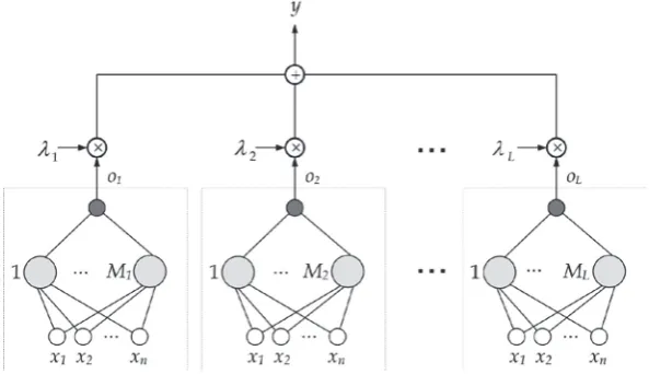
Figure 2 shows the linear combination scheme of ܮ
neural networks trained by OP-ELM. Note that the ܮ
networks have different hidden layer sizes and, in this approach, the feature input space is the same for all networks. The most appropiate models (with the same input feature space) are effectively chosen using OC-ELM. Whereas, when the OC-ELM-FFS approach is used, the input feature space is composed of the best ݀
attributes, with ݀ < ݊. Finally, in the case of the OC-ELM-RFS approach, the ܮ models have different random input subsets.
B. Ensemble design
Once the ܮdifferent ELMs have been trained, their network ouputs (ߧ) are previously ranked using the MRSR method [17] and the network output matrix ભ
is consequently ordered. Then, the better ܮכmodels are
chosen by minimizing the LOO error, which can be exactly measured with the PRESS statistic [20]. The inappropriate and useless models are discarded from the ensemble. This ensemble pruning reduces the storage needs, speeds up the operation stage and has the potential of improving the performance of the single neural architecture. It should be noted that the obtained ensemble system is fast and exact. Note that this stage is the same for the above three alternatives.
Finally, it should be noted that the model selection is exact and automatic. It is insensitive to random subsampling of validations sets (all samples are used for training and validation) and there is not any tuneable parameter.
([SHULPHQWV
A. Datasets
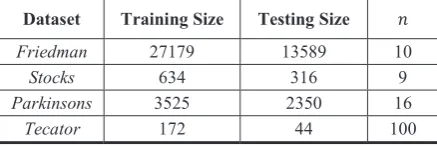
In order to evaluate the performance of the ELM methods discussed in this work, four well-known regression problems are studied. Table 1 summarizes these datasets.
7DEOHRegression datasets used in the experiments
'DWDVHW 7UDLQLQJ6L]H 7HVWLQJ6L]H ݊
Friedman 27179 13589 10
Stocks 634 316 9
Parkinsons 3525 2350 16
Tecator 172 44 100
The first two datasets (Friedman and Stocks) are from L. Torgo’s website [26], the Parkinsons dataset is obtained from UCI Machine Learning Repository [27] and the Tecator dataset is from the StatLib archive [28]. Except for Tecator (which is originally divided), each dataset is randomly splitted up into training () and test sets (). These regression problems have been selected trying to cover different complexities, such as large datasets or high dimensional data. The first dataset, Friedman, is an artificial problem and the three remaining benchmark prediction problems belong to different realworld scientific areas (economics, biomedical engineering and chemometrics).
xFriedman is a synthetic benchmark dataset. The input vectors are composed of ten attributes which have been independently generated following uniform distribution between 0and1. The target variable is computed by
10ݏ݅݊(ݔଵݔଶ) + 20ቀݔଷ െ1
2ቁ
ଶ
+ 10ݔସ+ 5ݔହ+ߪ ,
where ߪis a Gaussian white random noise with zero mean and unit variance. Then, the last five attributes are not relevant for predictions.
xStocks data contain daily stock prices from January 1988 through October 1991 for ten aerospace companies. The task is to predict the price of the 10thcompany given the prices of the rest.
xParkinsons dataset is composed of a range of biomedical voice measurements from 42 people with early-stage Parkinson’s disease recruited to a sixmonth trial of a telemonitoring device for remote symptom progression monitoring. There are 5785 voice recordings and each input vector has sixteen biomedical voice measures. From these variables, the main aim is to predict the UPDRS score, which is a rating scale used to follow the longitudinal course of Parkinson’s disease.
xTecator database consists of 215 near-infrared absorbance spectra of meat samples. Each observation consists of a 100-channel absorbance spectrum in the wave length range 850-1050 nm. The task is to predict the fat content of a meat sample on the basis of its near infrared absorbance spectrum.
B. Experimental results
Initially, the standard ELM algorithm and the OP-ELM method have been used for training individual SLFNs by considering that the hidden layer size (ܯ) is between 1and 150. The learning and testing phases are repeated ܮtimes (ܮdifferent weight initializations) in which the sigmoid function is selected as the activation function. In particular, ܮ= 50different repetitions have been done in all problems, except for Tecator because this highdimensional dataset requires more trials (ܮ= 100) in order to OC-ELM-FFS obtains different random networks with enough input feature diversity, as it has been already mentioned in the previous section. After that, the ensemble based approaches are validated. In particular, the ܮtrained OP-ELM networks are firstly combined by the least-squares solution of (8), i.e., the LSE-ELM method. Next, the three ensemble procedures (ELMs, OC-ELM-FFS and OC-ELM-RFS) are evaluated. Note that the OC-ELM method makes use of the same previously ܮ trained models with OP-ELM. In the experiments, all approaches use the LOO cross-validation technique, except for the standard ELM algorithm that uses 10-fold CV for selecting the hidden layer size. All simulations have been carried out in MATLAB 7.11(R2010b) environment running in the same machine with 4 GB of memory and 2.67 GHz processor.
that the RMSE of the ELM and OP-ELM methods are the best results of ܮtrials and, meanwhile, the results of the remaining approaches are given by the different ensemble schemes of the ܮ networks. In the last column of Table 2, the hidden layer sizes for the ELM and OP-ELM methods are shown and, meanwhile, the number of chosen networks is shown for the remaining ensemble-based approaches.
7DEOHExperimental results on four regression datasets
'DWDVHW /HDUQLQJ 0HWKRG 506( UHVXOWV 7UDLQLQJ 7LPHV 0RGHO VL]H Friedman ELM OP-ELM 2.67 2.64 7.87e+4 2.18e+3 139 99 LSE-ELM OC-ELM OC-ELM-FFS OC-ELM-RFS 2.38 2.38 1.44 1.28 2.26e+3 2.20e+3 5.47e+4 2.02e+3 50 30 16 33 Stocks ELM OP-ELM 1.11 1.11 2.46e+3 1.18e+2 141 101 LSE-ELM OC-ELM OC-ELM-FFS OC-ELM-RFS 0.81 0.78 0.74 0.72 1.19e+2 1.19e+2 2.30e+3 1.03e+2 50 24 16 18 Parkinsons ELM OP-ELM 9.02 9.59 1.07e+4 1.22e+3 139 85 LSE-ELM OC-ELM OC-ELM-FFS OC-ELM-RFS 8.97 8.95 9.02 8.87 1.23e+3 1.23e+3 6.40e+4 1.16e+3 50 20 9 39 Tecator ELM OP-ELM 4.88 3.57 8.25e+3 5.34e+2 76 67 LSE-ELM OC-ELM OC-ELM-FFS OC-ELM-RFS 2.45 2.28 1.28 2.04 5.40e+2 5.42e+2 1.07e+4 5.28e+2 100 43 15 29
With respect to relation between the dataset size and the required training time, two datasets can be compared: Tecator is a high dimensional dataset with a reduced number of samples and, in contrast, Friedman is defined by a large sample set with fewer input features. As it can be seen from Table 2, the required training time with Friedman (a large sample dataset) is longer than with Tecator (a small sample dataset). Therefore, according to these results, it can be said that the number of training samples is more determined on training time than the number of input features.
As it can be observed from Table 2, OP-ELM outperforms the ELM method by using more compact networks and less training time, except for Parkinsons dataset. With respect to the ensemble-based approaches, all of them provide better generalization capabilities than ELM and OP-ELM in all problems.
It is worthy of remark that these advantages are obtained with a negligible increment of the total training time with OP-ELM, except for the OC-ELM-FFS procedure which is based on incremental forward feature selection and, thus, it needs more
computational efforts. In all simulations, the OC-ELM-FFS and OC-ELM-RFS provide better results than the ensemble procedures based on the original input feature space. From these results, the use of random feature subsets is benefitial to the ensemble construction. This approach may be better than performing a previous forward feature selection, except for Tecator dataset. For example, in Tecator, the input data space is successfully reduced from one hundred to only five features with OC-ELM-FFS. Whereas, in Friedman dataset, although OC-ELM-FFS chooses the relevant features (which are previously known by the definition of this artificial dataset), this method achieves worse performance results than OC-ELM-RFS, which uses random feature subsets (including different combinations of relevant and irrelevant features). For the Parkinsons data, OC-ELM-FFS entails a high computational increment but the RMSE results are not improved. In this case, OC-ELM-RFS provides the best solution in terms of prediction accuracy. Note that OC-ELM-RFS requires, as expected, more networks to construct the ensemble than OC-ELM-FFS in all problems.
Therefore, according to these experimental results, it is recommended to exploit diversity in the ELM ensemble system by varying the input data space with random subsets and, also, a feature selection is clearly useful for high-dimensional datasets, prior to ensemble construction.
5
&RQFOXVLRQV
5HIHUHQFHV
[1] 6+D\NLQ Neural Networks: A Comprehensive Foundation (2ndEdition).Prentice Hall, July 1998.
[2] /.+DQVHQ 36DODPRQ Neural network ensem-bles. In: IEEE Transactions on Pattern Analysis and Machine Intelligence, 1990, Vol. 12, No. 10, pp. 993-1001.
[3] 0)0ROOHU “Diversity in neural network ensem-bles,” Ph.D. dissertation, University of Birmingham, 2003.
[4] $/LSQLFNDV Adaptive committes of neural classifiers. In: Information Technology and Control, 2008, Vol. 37, No. 3, pp. 205–210.
[5] 61DEDYL.HUL]L 0$EDGL (.DELUA PSO-based weighting method for linear combination of neural networks. In: Computers & Electrical Engineering, 2010, Vol. 36, No. 5, pp. 886–894.
[6] *+XDQJ 4=KX &6LHZ Extreme learning machine: a new learning scheme of feedforward neural networks. In:IEEE International Joint Conference on Neural Networks, 2004, Vol. 2, pp. 985–990.
[7] *+XDQJ4=KX&6LHZExtreme learning machi-ne: Theory and applications. In: Neurocomputing, 2006, Vol. 70, No. 1-3, pp. 489–501.
[8] *%+XDQJ '+:DQJ </DQExtreme learning machines: A survey. In: International Journal of Machine Leaning and Cybernetics, 2011, Vol. 2, No. 2, pp. 107–122.
[9] 3- *DUFtD/DHQFLQD $ %XHQR&UHVSR -/6DQFKR*yPH] Neurocomputing: Learning, Architectures and Modelings. Nova Science, 2012, ch. 6. Design and Training of Neural Architectures using Extreme Learning Machines, pp. 119–145.
[10]<0LFKH $6RUMDPDD 3%DV 26LPXOD &-XWWHQ $/HQGDVVHOP-ELM: Optimally Pruned Extreme Learning Machine. In: IEEE Transactions on Neural Networks, 2010, Vol. 21, No. 1, pp. 158–162. [11]&55DR 6.0LWUD Generalized Inverse of
Matrices and its Applications. New York: Wiley, 1971. [12]*%+XDQJ /&KHQ &.6LHZUniversal appro-ximation using incremental constructive feedforward networks with random hidden nodes. In: IEEE Transactions on Neural Networks, 2006, Vol. 17, No. 4, pp. 879–892.
[13]*%+XDQJ 0%/L /&KHQ &.6LHZ Incremental extreme learning machine with fully complex hidden nodes. In: Neurocomputing, 2008, Vol. 71, pp. 576–583.
[14]*%+XDQJ/&KHQEnhanced random search based incremental extreme learning machine. In:
Neurocomputing, 2008, Vol. 71, pp. 3460–3468. [15]+-5RQJ <62QJ $+7DQ ==KX A fast
prunedextreme learning machine for classification problem. In: Neurocomputing, 2008, Vol. 72, No. 1-3, pp. 359–366.
[16]<0LFKH3%DV&-XWWHQ26LPXOD$/HQGDVVH. A methodology for building regression models using extreme learning machine: OP-ELM. In Proceedings of the European Symposium on Artificial Neural Networks (ESANN), 2008, pp. 247–252.
[17]76LPLOl -7LNND Multiresponse sparse regression with application to multidimensional scaling. In
Proceedings of the 15th International Conference on Artificial Neural Networks: Formal Models and Their Applications - ICANN 2005, ser. LNCS 3697, 2005, pp. 97–102.
[18]%(IURQ 7+DVWLH /-RKQVWRQH 57LEVKLUDQL Least angle regression. In:Annals of Statistics, 2004, Vol. 32, pp. 407–499.
[19]$%DUWROL On computing the prediction sum of squares statistic in linear least squares problems with multiple parameter or measurement sets. In:
International Journal on Computer Vision, November 2009, Vol. 85, pp. 133–142.
[20]50\HUV Classical and Modern Regression with Applications, 2nd ed. Duxbury Press, 1990.
[21]</DQ <6RK *%+XDQJ Ensemble of online sequential extreme learning machine. In:
Neurocomputing, 2009, Vol. 72, No. 13-15, pp. 3391-3395.
[22]1/LX +:DQJ Ensemble based extreme learning machine. In: IEEE Signal Processing Letters, 2010, Vol. 17, No. 8, pp. 754 –757.
[23]+&KHQ +&KHQ ;1LDQ 3/LX Ensembling extreme learning machines. In: 4th International Symposium on Neural Networks, ISNN, 2007, pp. 1069–1076.
[24]09DQ +HHVZLMN <0LFKH 7/LQGK.QXXWLOD 3+LOEHUV 7+RQNHOD (2MD $/HQGDVVH Adaptive ensemble models of extreme learning machines for time series prediction. In: International Conference on Artificial Neural Networks, ser. LNCS, Vol. 5769, No. July, 2009, pp. 305–314.
[25]0YDQ +HHVZLMN <0LFKH (2MD $/HQGDVVH Solving large regression problems using an ensemble of GPU-accelerated ELMs. In: ESANN2010: 18th European Symposium on Artificial Neural Networks, Computational Intelligence and Machine Learning, 2010, pp. 309–314.
[26]/7RUJRRegression datasets. [Online]. Available at: http://www.liaad.up.pt/ltorgo/Regression/DataSets.html. [27]$$VXQFLRQ '1HZPDQ UCI machine learning
repository. [Online]. Available at: http://www.ics.uci.edu/~mlearn/MLRepository.html.
[28]39ODFKRV Statlib archive. [Online]. Available at: http://lib.stat.cmu.edu.
[29]==KDR <=KDQJ +/LDR Design of ensemble neural network using the akaike information criterion. In: Engineering Applications of Artificial Intelligence, Vol. 21, No. 8, 2008, pp. 1182–1188.