Copyright © 2015 IJECCE, All right reserved
Delay and Non-Delay Differential Models of Diabetes
Type 1
Dr. Maysoon M.Aziz
Department of mathematics
College of Computer Science and Mathematics Mosul University, Mosul-Iraq Email: [email protected]
Zahraa A. Al-Nuaimi
Department of Operation Research Intelligent Technology College of Computer Science and Mathematics
Mosul University, Mosul-Iraq Email: Zahraa [email protected]
Abstract – Mathematical models (ratio-dependent) for two systems, One without time delay and the second with time delay.It was found that the two models are stable.
Keywords – Diabetes, Lyapunov, Stability, New Method, Fixed Points, Delay Differential Equations Hopf- Bifurcation.
I.
I
NTRODUCTIONThe complete name of the disease is Diabetes mellitus. Diabetes is derived from the Greek word for “passing through”, and mellitus from the Latin word “honey”, referring to the excessive sugar in the urine of the patients [9].
Diabetes combines a group of different metabolic disorders, which have different origins, but all resulting in hyperglycemia or high blood glucose levels. Insulin is needed by the cells as a mediator for glucose uptake. High blood glucose levels are mainly caused by a deficiency or a resistance to available [3].
Diabetes mellitus is a group of Metabolic diseases characterized by elevated blood glucose levels (hyperglycemia) resulting from defects in insulin secretion, insulin action or both [17].
Insulin is a hormone manufactured by the -cell of the Pancreas which is required to utilize glucose from digested food as an energy source [17].
Chronic hyperglycemia is associated with microvaular and microvascular complications that can leads to visual impairment blindness, kidney disease, nerve damage,amputations, heart disease, and stroke.
The type of diabetes is based on the presumed etiology. Type 1 diabetes is characterized by a significant, often sudden deficiency of insulin.
It is caused by an auto-immune disorder destroying the insulin producing -cells in the pancreas and has a strong genetic pre-disposition. This type of diabetes is commonly known as juvenile-onset diabetes, but can also strike adults and is not linked to obesity About 10% of people with diabetes have type 1[3].
In type 1 diabetes, the body does not produce insulin and daily insulin injection are required.
Type 1 diabetes is usually diagnosed during childhood or early adolescence.
Type 2 diabetes is the result of failure to produce sufficient insulin and insulin resistance.
Most people who develop type 1 diabetes do not have a family history of the disease. The odds of inheriting the disease are only 10% if a first-degree relative has diabetes and, even in identical twins, one twin has only a 33%
chance of having type 1 diabetes if the other twin has it. Children are more likely to inherit the disease from a father with type 1 diabetes than from a mother with the disorder.
Genetic factors cannot fully explain the development of diabetes. For the past several decades, the number of new cases of type 1 diabetes has been increasing each year worldwide [18].
Delay differential equations (DDEs) have been used as mathematical models in many areas of Biology and Medicine. Such areas include Epidemiology, Population Biology, Immunology, Physiology, Cell mobility.
Delayed effects often exist in the glucose-insulin regulatory system, for example, the insulin secretion stimulated by elevated glucose concentration level, hepatic glucose production.
Therefore the delays need to be taken into account when modeling the systems [5].
The new method is useful way because it used with linear and non-linear system and this way merge two ways [19].
II.
T
HEM
ATHEMATICALM
ODELS(R
ATIO–
D
EPENDENT)
[15]
The First Model (ratio-dependent) is with second type of functional response [6].
1 1
-dy
dx x cxy
ex
dt k my x
dy sxy dt my x
Where x(t) is represents a measure of sugar in the blood (mg/dl) , y(t) is the insulin dose given (Um) , b is the birth rate , d is the death rate , e is the growth rate ,(not strict growth rate because instrict growth rate calculated when the predator is absent)[15]. s is the conversation rate. The
capturing rate (functional response) is given by
x
m
cx
where m is the half saturation constant (m=0.5*c), c is the maximal growth rate.
We use this formula of functional response because the population growth is logistic [15].The equations of (b, d, e,b1) are given by [7], such that
number of births
*1000 population mid year
b
number of total deaths *1000 population mid year
Copyright © 2015 IJECCE, All right reserved
*1000 population mid year
b d
e
From our set of data in appendix (1) we get b=35.5157, d=4.1869, e=31.3128
n
x
b
a
s
x
b
y
a
x
n
x
y
x
n
xy
b
n
i
1 1 1
2 2 1
[10]
From our set of data in appendix (3) we get, a=16.558, b1=0.922, s=29.4331
The matrix representation of the system (1) is given by
1869
.
4
1648
.
1
571
.
1
4355
.
0
A
The characteristic equation of the system is λ2
+ 3.7514λ+ 0.00650585 = 0 (2) The eigenvalues of the matrix A are
7497
.
3
0017
.
0
21
Since the two eigenvalues are negative, so the system is stable
II.
A
NALYSIS OFS
TABILITYT
ESTM
ETHODS2-1- Routh –Array criteria, [1], [8] for first model.
The Routh stability test states that the system is asymptotically stable ((all poles in OLPH ((open left half plane)) iff all the elements in the first column of the Routh array are strictly positive (>0).In addition the number of poles not in the OLPH is equal to the number of sign changes in the first column.𝑎0= 0.00650585, 𝑎1= 3.7514, 𝑎2= 1
Table 1: Routh Array for System (1)
2
11
3.7514 00
0.00650585 0Since a0,a1>0 and a2>0 there is no change in the sign in
the first column ,so the poles are in the OLHP (open left half plane).
Therefore, the system (1) is stable.
2-2 Hwritz-Criteria [2].
This criteria is to test if the system is stable or not.If the principal minors of the square matrixAof the system are all positive then the system is stable, otherwise it's unstable. If n=2(where n denote the degree of the square matrix)
3 2
1 2 1
1
,
a
a
na
na
na
nFrom equation (2) we find
𝛥1= 3.7514 > 0, 𝛥2= 𝑎1𝑎0= 0.0244 > 0
The system (1) is stable.
2-3 Lyapunov Stability: [10].
The system is stable if the following are satisfies
n
-I
Q
,
A
P
PA
Q
X
T0
T
Q Q (3)
Where Inis the identity matrix, and A is the matrix of the system (3)
P is positive definite (P is the lyapunov matrix of the matrix A) (i.e. the values of eigenvalues must greater than zero).
By using a designed program(1) in Matlabwe get
5809
.
54
1462
.
145
1462
.
145
0639
.
387
P
Where P is the Lyapunov matrix of the original matrix A, the eigenvalues of P
0
5114
.
441
,
0
133
.
0
2P1
PWhich makes the matrix P positive definite matrix (i.e. all eigenvalues must greater than zero).
We find
1
0
0
1
2
I
PA
P
A
X
TAlthough the equation (3) satisfies, therefore the system is stable.
Program (1)
A=input ('A=')
Q= [1 0; 0 1]; P=lyap (A', Q) Lamda= eig (P) X=A'*P+P*A
Note1: the system is asymptotically stable if the eigenvalues of the system have negative real parts. The eigenvalues of the matrix A are
7497
.
3
0017
.
0
21
Since we have two eigenvalues less than zero, therefore the system is asymptotically stable
Theorem 1: [13]
The time invariant system is asymptotically stable iff the pair (A, C) is observable and the equation (3) having a unique positive definite solution. By using a designed program (2) in MATLAB we get
𝑃1= 27.7956 − 10.3923 −10.3923 4.0188 The pair (A, C) is observable
And the eigenvalues of the matrix P𝟏 are 𝜆1𝑝1 = 0.1169 > 0, 𝜆2𝑝1= 31.6975 > 0
Program (2)
A=input ('A=')
b=rank(A) C= [0 1]; Q1=C'*C
y=lyap (A', Q1) g=rank(Y)
If ('g=b')
Disp ('the pair (A, c) is observable')
End
Copyright © 2015 IJECCE, All right reserved Since the matrix P1 is positive definite, therefore the
systems is stable.
2-4- Lyapunov Function [13].
We use quadratic function for our model. We assume that
2 2,
y
x
y
x
V
,
8
dt
dy
y
v
dt
dx
x
v
y
x
V
𝐼𝑓𝑉 𝑥, 𝑦 < 0 Thenthesystemisstable 12 2
( , ) 2 (31.3128 35.5157
11.045 29.4331
) 2 ( 4.1869 )
21.672 21.6742
V x y x x x
xy xy
y y
y x y x
(4)
)
3738
.
8
0314
.
71
6256
.
62
(
))
6742
.
21
09
.
29
8662
.
58
(
(
,
2 3 2
y
x
x
x
y
y
x
xy
y
x
V
By using equation (4) and the set of our real data in appendix (2) we get
x
,
y
0
V
, so the system (1) is stable.2-5 Continued Fraction Stability Criteria [2].
The criterion is applied to the characteristic equation (1) of a continuous system by forming a continued fraction from the odd and even portions of the equation.
6224 . 4 0069008 . 0 2 2 1 Q QFrom the fractionQ1/Q2, and then divide the denominator into the numerator and invert the remainder, to form a continued fraction as follows:
6224
.
4
0069008
.
0
6624
.
4
1
0 21
Q
Q
2 11
h
h
If all values of (
h
1,
h
2) positive, then the roots of0
)
(
Q
have negative real parts. (The system is stable) Since,0
00149
.
0
h
,
0
6624
.
4
1
21
h
The system is stable.
2-6 New Method for Constructing Lyapuov
Function [15].
Step1: apply continued fracture criteria to create the factors of the characteristic polynomial
n nn n n
a
a
a
a
a
p
1
2 2 1 1
0
..
Step 2: construct Lyapunov function as
n j j jx
h
x
V
0 24
1
From the paragraph (2-5) we have,
0133
.
0
h
,
0319
.
0
21
h
We assume the lyapunov function as
2 2 1 2 1 2 1 , 4 1, 2 2
4
V x y h x h y V x y h xx h yy
13.527 15.347 0.01247
(5)) 6742 . 21 77144 . 4 0877 . 0 ( ( 2 1 3 2 y x x x y y x xy
By using equation (5) and the set of our real data in appendix (2) we get
x
,
y
0
V
, so the system (1) is stable.2-7 Test the Stability by Using the Fixed Points:
(This way is used for nonlinear system).Given a system of ODEs,(ordinary differtional equations) steady state values can be found by setting all time derivatives equal to zero and solving
2
dx cxy
ex bx
dt my x
dy sxy
dy
dt my x
Now, for steady state
0
,
0
dt
dy
dt
dx
By solving above equations we get two fixed points (0, 0), (0.8694, 0.2419)
The Jacobian matrix of the system at (0,0) is given as
1869
.
4
0
0
5147
.
35
J
The eigenvalues of J are
1869
.
4
5147
.
35
JJ
The Jacobian matrix at, (0.8694, 0.2419)is given by
5914
.
3
9991
.
0
2235
.
0
8168
.
30
J
The eigenvalues as follows
5996
.
3
8086
.
30
2 1
J J
Then the system is stable in (0.00454, 1.2066) The fixed points of above system are
(0, 0), (0.8694, 0.2419),(0.8779,0)
The Jacobian matrix of above system at (0.8779, 0) is given by
2462
.
25
0
045
.
11
21
.
241
1
J
The eigenvalues as follows
25.2462 241.2100 -2 , 1 1 , 1 J J
Since the trace of J1=-215.96
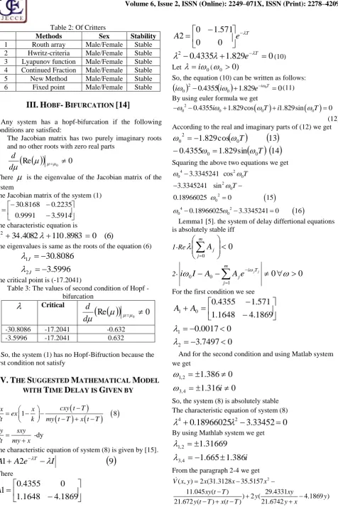
Copyright © 2015 IJECCE, All right reserved Table 2: Of Critters
Methods Sex Stability
1 Routh array Male/Female Stable 2 Hwritz-criteria Male/Female Stable 3 Lyapunov function Male/Female Stable 4 Continued Fraction Male/Female Stable 5 New Method Male/Female Stable 6 Fixed point Male/Female Stable
III.
H
OBF-
B
IFURCATION[14]
Any system has a hopf-bifurcation if the following conditions are satisfied:
1. The Jacobian matrix has two purely imaginary roots and no other roots with zero real parts
2.
Re
0
0
d
d
Where
is the eigenvalue of the Jacobian matrix of the systemThe Jacobian matrix of the system (1)
5914 . 3 9991 . 0
2235 . 0 8168 . 30
J
The characteristic equation is
(6)
0
8983
.
110
4082
.
34
2
The eigenvalues is same as the roots of the equation (6)
5996
.
3
8086
.
30
2 1
J J
The critical point is (-17.2041)
Table 3: The values of second condition of Hopf -bifurcation
Critical
Re
0
0
d
d
-30.8086 -17.2041 -0.632
-3.5996 -17.2041 0.632
So, the system (1) has no Hopf-Bifruction because the first condition not satisfy
IV.
T
HES
UGGESTEDM
ATHEMATICALM
ODEL WITHT
IMED
ELAY ISG
IVEN BY
1 8
-dy cxy t T
dx x
ex
dt k my t T x t T
dy sxy dt my x
The characteristic equation of system (8) is given by [15].
9
2
1
A
e
I
A
T
Where
1869
.
4
1648
.
1
0
4355
.
0
1
A
T
e
A
0
0
571
.
1
0
2
0
829
.
1
4335
.
0
2
T
e
(10)Let
i
0(
0
0
)
So, the equation (10) can be written as follows:
0.4355
1.829 0 00 2
0
i T
e i
i
(11)By using euler formula we get
2
0 0.4355i 0 1.829 cos 0T i1.829sin 0T 0
(12) According to the real and imaginary parts of (12) we get
14
sin
829
.
1
4355
.
0
13
cos
829
.
1
0 0
0 2
0
T
T
Squaring the above two equations we get
4 2
0 0
2 0 2 0
3.3345241 cos 3.3345241 sin
0.18966025 0 15
T T
4 2
0 0.18966025 0 3.3345241 0 16
Lemma1 [5]. the system of delay differtional equations is absolutely stable iff
1-Re
0
0
mj j
A
2-
0
0
1 0
0
m j
T i j
j j
e
A
A
I
i
For the first condition we see
1869
.
4
1648
.
1
571
.
1
4355
.
0
0
1
A
A
0
7497
.
3
0
0017
.
0
2 1
And for the second condition and using Matlab system we get
0
316
.
1
0
386
.
1
4 , 3
2 , 1
i
So, the system (8) is absolutely stable The characteristic equation of system (8)
0
33452
.
3
18966025
.
0
24
By using Mathlab system we get
i
386
.
1
665
.
1
31669
.
1
4 , 3
2 , 1
From the paragraph 2-4 we get 2 ( , ) 2 (31.3128 35.5157
11.045 ( ) 29.4331
) 2 ( 4.1869 )
21.672 ( ) ( ) 21.6742
V x y x x x
xy t T xy
y y
y t T x t T y x
Copyright © 2015 IJECCE, All right reserved
2 3
2
58.8662 29.09
( ( ))
21.6742
(62.6256 71.0314
, 19
8.3738 )
22.09
21.6742
x y
xy
y x
x x
V x y
y
xy t T
y t T x t T
By using equation (19) and the set of our real data in appendix (2) we get
x
,
y
0
V
,so the system (8) is stable Test the Stability by Using the Fixed Points: (This way is used for nonlinear system).Given a system of ODEs,(ordinary differtional equations) steady state values can be found by setting all time derivatives equal to zero and solving
)
(
)
(
)
(
2
x
my
sxy
dy
dt
dy
T
t
x
T
t
my
T
t
cxy
bx
ex
dt
dx
For steady state
0
,
0
dt
dy
dt
dx
By solving above equations we get two fixed points (0, 0), (0.8694,0.2419) (the equilibrium points of time delay are same as without time delay)
The jacobain matrix
5914 . 3 9991 . 0
2235 . 0 8168 . 30
J +
e
T
0
0
223
.
0
0622
.
0
The characteristic equation of the Jacobian matrix is given by
0
829
.
1
4335
.
0
2
T
e
(20)The final equation as follows
0
868
.
1409130
45
.
1163
24
207
.
27
63
.
43
4 , 3
2 , 1
i
By using the lemma1
The system is absolualty stable
V.
H
OBF-
B
IFURCATION[14]
From the above paragraph we see the first condition of Hobf-bifruction is not satisfied
The critical points are (0,
581
.
725
i
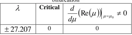
)Table 4: The values of second condition of Hopf -bifurcation
Critical
Re
0
0
d
d
207
.
27
0 0The second condition is not satisfied So, the system has no hobf-bifruction.
VI.
C
ONCLUSIONIn this paper, we found that: 1. The two models are stable.
2. The two models have no hopf-bifurcation
R
EFERENCES[1] Kaman, E., Introduction to signal and Systems.macmillan Publishing company (1987)
[2] Joseph J, Allen, Ivan Feedback and Control Systems. McGraw-Hill (1990)
[3] Thomas Lotz" Model-Based Assessment ofInsulin Sensitivity" thesis, University of Canterbury, Christchurch, New Zealand (2007)
[4] Howard Modeling Basics .Fall (2009)
[5] S.ruan "On non-linear Dynamics of Predatot-Prey Models with Discrete Delay ''Math. Model. Nat. Phenom. Vol. 4, No. 2, 2009, pp. 140-188
[6] K Visweswara Rao.Biostatistics in Brief Made Easy Jaypee Brothers Medical PublishersLtd., NewDelhi (2010)
[7] Boccara,N."Modeling Complex Systems" Springer (2010) [8] Singh, N , Beniwal, R Automatic control systems with matlab
programming Merha Offset Press ,Delhi (2010)
[9] Diagnosis and classification of Diabetes Mellitus, U.S National library of Medicin, National Institutes of Health, Jan (2010) [10] A.A.Martynyuk, Stability by Liapunov’s Matarcel Functions
Methods with Application.New York Marcel Dekker, (2011) [11] Douglas C.Montgomery, George C.Runger Applied Statistics
and Engineering John Wiley (2011)
[12] Wan-Yang wang.Li-JunPei: Stability and Hopfbifurcation of a delay ratio –dependent predator-prey system .Acta Mech.Sin (2011)
[13] Chutiphon Pukdeboon''A review of Fundamental of Lyapunov Theory'"the Journal of Applied Science vol.10 No.2 (2011) [14] Rebort,M." Introduction to Bifurcation and the Hopf Bifurcation
Theorem for Planar Systems"Department of Mathematics, Colorado University (2011)
[15] Wan-Yong Wang.Li-Jun Pei"stability and Hopf bifruction of a delayed ration dependent predator –prey system'" acta Mech.Sin (2011)
[16] Li Hongweiademy of science, Engineering and "Hopf bifruction of a predator-prey model with time delay and habitat complexity', World Academy of science, Engineering and technology ,vol:60 2011-12-22
[17] Stang J, Story M (eds) Guidelines for Adolescent Nutrition Services (2013)
[18] www. Diabetes - type 1 |University of Maryland Medical Center (2013)
[19] Aziz, zahraa "Stability and Hopf-Bifurcation For Diabetes Model" International Journal of Electronics Communication and Computer Engineering (IJECCE) vol.4, Issue 3, May (2013)
A
UTHOR’
SP
ROFILEDr. Maysoon A. Aziz
Ph.D., Department of Mathematics,College of computer science and mathematics, Mosul University Iraq.
Mathematical Methods and Time Series, Mosul University. M.Sc. MathematicalStatistics, Sussex University, England,. Email: [email protected]
Zahraa A. Al-Nuaimi
Copyright © 2015 IJECCE, All right reserved
A
PPENDIXAppendix (1)
Population mid year growth rate
Deaths Births
Years
865500.00 17.65
2884.00 15277.00
1973.00 1.
883000.00 18.69
2975.00 16503.00
1974.00 2.
900500.00 18.82
2157.00 16945.00
1975.00 3.
917828.00 26.88
4084.46 24672.82
1976.00 4.
935488.00 28.80
4264.16 26941.14
1977.00 5.
953377.00 33.59
4581.00 32026.00
1978.00 6.
971664.50 34.21
4911.00 33238.00
1979.00 7.
990302.50 33.89
5185.00 33563.00
1980.00 8.
1009298.00 35.23
5500.00 35555.00
1981.00 9.
1028657.50 34.19
5162.70 35172.00
1982.00 10.
1048388.50 35.62
5691.00 37344.00
1983.00 11.
1068498.50 36.34
6222.00 38833.00
1984.00 12.
1218365.50 35.90
5743.00 43741.00
1985.00 13.
1375431.00 33.54
6149.00 46132.00
1986.00 14.
1436105.00 33.84
5778.00 48600.00
1987.00 15.
1473478.00 34.11
6114.00 50255.00
1988.00 16.
1524017.00 39.10
6592.00 59585.00
1989.00 17.
1572354.00 44.37
7089.00 69762.00
1990.00 18.
1591450.00 38.46
6986.00 61205.00
1991.00 19.
1645750.00 44.66
7839.00 73499.00
1992.00 20.
1700200.00 48.19
8241.00 81941.00
1993.00 21.
1754700.00 43.63
8144.00 76561.00
1994.00 22.
1809050.00 38.41
7773.00 69492.00
1995.00 23.
1864383.50 38.32
7393.00 71444.00
1996.00 24.
1927433.50 37.55
7811.00 72371.00
1997.00 25.
1985687.00 32.26
7794.00 64067.00
1998.00 26.
2048937.00 31.91
7671.00 65386.00
1999.00 27.
2120550.00 35.45
7648.00 75163.00
2000.00 28.
2183583.50 36.26
7886.00 79181.00
2001.00 29.
2247896.50 37.35
8763.00 83969.00
2002.00 30.
2314734.50 30.13
7925.00 69740.00
2003.00 31.
2451456.50 34.15
8704.00 83717.00
2004.00 32.
2595798.50 34.25
10180.00 88916.00
2005.00 33.
2680128.50 36.99
11478.00 99137.00
2006.00 34.
2767010.50 34.52
12431.00 95526.00
2007.00 35.
2918606.00 40.11
11087.00 117067.00
2008.00 36.
3036957.50 42.80
10486.00 130244.00
2009.00 37.
3169202.50 41.80
3970.00 137765.00
2010.00 38.
3280516.50 41.00
10374.20 104064.07
2011.00 39.
3302811.00 40.00
10553.90 106332.39
2012.00 40.
Appendix (2)
Raw data of 581 patients including (sex, age, bloodsugar, in insulin dose)
Sex Age Blood
Sugar
Insulin Dose 1. Female 24.00 17.70 54.00 2. Male 36.00 11.40 90.00 3. female 20.00 19.10 70.00 4. female 20.00 16.40 60.00 5. female 25.00 11.90 45.00 6. Male 31.00 11.00 70.00 7. Male 35.00 8.40 30.00
Sex Age Blood
Sugar
Copyright © 2015 IJECCE, All right reserved
Sex Age Blood
Sugar
Insulin Dose 19. female 20.00 13.50 60.00 20. female 25.00 5.70 25.00 21. female 10.00 7.70 36.00 22. female 25.00 6.22 13.00 23. female 21.00 8.50 12.00 24. male 6.00 31.00 6.00 25. female 16.00 20.40 28.00 26. male 38.00 12.40 55.00 27. male 35.00 21.60 30.00 28. male 9.00 17.20 30.00 29. male 23.00 27.00 75.00 30. male 11.00 6.40 32.00 31. male 10.00 10.00 30.00 32. female 40.00 5.10 10.00 33. female 17.00 15.40 35.00 34. male 10.00 5.80 20.00 35. female 35.00 7.90 38.00 36. male 8.00 24.00 35.00 37. female 19.00 18.10 90.00 38. female 28.00 12.80 25.00 39. female 14.00 15.40 65.00 40. male 21.00 17.20 20.00 41. male 39.00 9.10 48.00 42. male 9.00 16.90 40.00 43. female 4.00 6.94 6.00 44. female 31.00 15.20 60.00 45. female 29.00 5.30 55.00 46. male 36.00 6.50 8.00 47. male 36.00 3.30 27.00 48. male 31.00 6.70 46.00 49. male 40.00 14.00 45.00 50. female 14.00 16.30 50.00 51. female 26.00 18.80 25.00 52. male 10.00 16.50 67.00 53. male 31.00 27.70 50.00 54. female 30.00 16.20 45.00 55. female 29.00 8.80 73.00 56. male 14.00 8.10 48.00 57. female 18.00 14.00 25.00 58. female 23.00 15.50 50.00 59. male 21.00 13.60 50.00 60. female 28.00 16.70 75.00 61. male 12.00 17.40 55.00 62. male 33.00 7.50 71.00 63. female 20.00 14.70 80.00 64. female 19.00 14.30 15.00 65. female 30.00 5.80 15.00 66. female 12.00 3.70 46.00 67. female 31.00 7.40 51.00 68. female 15.00 7.40 30.00 69. female 19.00 6.40 40.00 70. female 20.00 12.00 58.00 71. male 24.00 15.80 60.00 72. male 36.00 6.00 50.00 73. female 24.00 17.20 30.00 74. female 19.00 11.00 40.00
Sex Age Blood
Sugar
Insulin Dose 75. male 22.00 11.00 40.00 76. male 27.00 15.70 60.00 77. female 34.00 16.90 60.00 78. female 34.00 16.34 65.00
79. male 1.00 2.20 3.00
80. male 19.00 6.70 65.00 81. female 24.00 4.90 41.00 82. female 40.00 5.50 50.00 83. female 28.00 4.00 25.00 84. female 26.00 13.40 25.00 85. female 29.00 8.80 73.00 86. male 17.00 7.60 70.00 87. female 33.00 14.40 45.00 88. female 19.00 8.80 50.00 89. male 11.00 25.90 35.00 90. male 21.00 17.10 45.00 91. female 29.00 16.70 95.00 92. male 15.00 17.40 55.00 93. female 20.00 12.00 50.00
94. male 1.00 2.20 3.00
Copyright © 2015 IJECCE, All right reserved
Sex Age Blood
Sugar
Insulin Dose 131. male 29.00 17.00 65.00 132. male 13.00 18.10 45.00 133. female 35.00 7.10 34.00 134. female 21.00 16.70 45.00 135. female 24.00 19.70 55.00 136. male 25.00 15.80 80.00 137. female 28.00 12.50 45.00 138. female 9.00 19.44 26.00 139. female 14.00 6.20 19.00 140. male 16.00 22.80 65.00 141. female 14.00 19.80 36.00 142. male 21.00 15.00 60.00 143. male 27.00 12.20 48.00 144. male 28.00 10.70 30.00 145. male 27.00 13.80 30.00 146. female 31.00 5.50 75.00 147. female 40.00 7.50 30.00 148. female 36.00 7.90 53.00 149. female 3.00 11.16 4.00 150. female 33.00 7.40 20.00 151. female 39.00 10.70 45.00 152. male 34.00 6.20 30.00 153. male 33.00 9.70 34.00 154. female 28.00 20.70 85.00 155. female 33.00 17.80 30.00 156. female 22.00 20.44 60.00 157. male 38.00 25.90 60.00 158. male 20.00 15.40 75.00 159. female 16.00 17.30 110.00 160. female 21.00 20.60 80.00 161. male 27.00 25.00 55.00 162. male 23.00 7.50 40.00 163. male 35.00 12.00 50.00 164. male 23.00 13.30 55.00 165. female 22.00 20.70 47.00 166. female 29.00 11.60 75.00 167. female 28.00 13.00 80.00 168. female 19.00 17.40 55.00 169. male 23.00 19.40 55.00 170. male 24.00 10.80 45.00 171. male 20.00 21.60 50.00 172. female 28.00 11.00 40.00 173. female 24.00 15.80 60.00 174. female 34.00 26.40 55.00 175. female 25.00 5.60 60.00 176. female 31.00 3.20 106.00 177. male 24.00 22.90 75.00 178. male 10.00 3.10 26.00 179. male 35.00 16.40 40.00 180. male 23.00 18.70 50.00 181. male 19.00 14.70 45.00 182. female 25.00 20.21 50.00 183. female 33.00 8.80 208.00 184. male 29.00 15.90 80.00 185. female 24.00 12.10 50.00 186. female 21.00 9.10 36.00
Sex Age Blood
Sugar
Copyright © 2015 IJECCE, All right reserved
Sex Age Blood
Sugar
Insulin Dose 243. female 25.00 7.10 37.00 244. male 32.00 21.10 60.00 245. male 23.00 9.60 35.00 246. female 31.00 10.80 80.00 247. male 37.00 12.00 34.00 248. male 5.00 8.33 22.00 249. female 14.00 21.30 45.00 250. female 31.00 4.70 89.00 251. male 8.00 5.50 17.00 252. male 11.00 7.20 19.00 253. female 10.00 9.50 34.00 254. male 24.00 5.10 70.00 255. female 40.00 6.10 20.00 256. male 13.00 6.67 28.00 257. male 35.00 20.50 40.00 258. female 32.00 27.39 60.00 259. female 37.00 18.16 60.00 260. female 4.00 5.00 12.00 261. male 36.00 16.30 30.00 262. male 14.00 10.00 30.00 263. female 23.00 11.30 50.00 264. female 29.00 30.50 40.00 265. male 12.00 18.40 15.00 266. female 9.00 6.20 24.00 267. male 14.00 21.30 30.00 268. male 19.00 18.30 25.00 269. Female 37.00 7.90 40.00 270. Male 27.00 11.33 45.00 271. Female 24.00 8.20 15.00 272. Female 33.00 7.22 79.00 273. Male 7.00 18.00 32.00 274. Female 11.00 26.56 27.00 275. Male 21.00 14.30 60.00 276. Female 10.00 10.80 40.00 277. male 36.00 23.60 100.00 278. male 9.00 27.80 21.00 279. male 12.00 12.80 25.00 280. female 40.00 5.40 65.00 281. male 23.00 17.00 55.00 282. male 17.00 9.27 45.00 283. male 13.00 5.10 42.00 284. female 20.00 7.90 50.00 285. female 13.00 19.20 42.00 286. male 35.00 21.22 57.00 287. male 19.00 5.40 30.00 288. female 9.00 14.80 34.00 289. male 38.00 26.70 70.00 290. male 30.00 6.39 27.00 291. male 37.00 27.70 30.00 292. female 16.00 5.70 61.00 293. male 29.00 15.00 32.00 294. male 21.00 13.89 30.00 295. female 16.00 11.00 40.00 296. male 30.00 19.10 24.00 297. female 37.00 8.10 60.00 298. female 30.00 22.80 32.00
Sex Age Blood
Sugar
Copyright © 2015 IJECCE, All right reserved
Sex Age Blood
Sugar
Insulin Dose 355. Female 37.00 26.50 70.00 356. Male 32.00 21.20 55.00 357. Female 17.00 3.70 71.00 358. Female 18.00 27.20 25.00 359. Male 4.00 5.70 67.00 360. Female 31.00 24.20 60.00 361. Female 39.00 9.20 60.00 362. Male 22.00 5.50 60.00 363. Male 23.00 11.60 50.00 364. Female 17.00 8.60 65.00 365. Female 22.00 17.90 80.00 366. Female 33.00 7.60 110.00 367. Male 30.00 16.40 17.00 368. Male 31.00 17.80 70.00 369. Male 18.00 7.60 65.00 370. Female 28.00 10.80 40.00 371. Male 35.00 24.20 40.00 372. Female 5.00 3.50 8.00 373. Male 8.00 18.00 60.00 374. Male 14.00 8.80 25.00 375. Male 30.00 27.50 30.00 376. Male 34.00 6.90 40.00 377. Male 40.00 16.50 15.00 378. Male 15.00 26.60 52.00 379. Female 2.00 11.11 3.00 380. female 37.00 10.50 57.00 381. female 31.00 17.60 30.00 382. female 37.00 19.30 55.00 383. male 28.00 13.50 80.00 384. male 21.00 11.40 30.00 385. male 20.00 18.20 50.00 386. female 24.00 4.50 30.00 387. female 31.00 5.90 88.00 388. male 21.00 10.00 47.00 389. female 39.00 6.80 25.00 390. male 20.00 11.61 45.00 391. male 40.00 7.70 70.00 392. female 13.00 9.40 58.00 393. female 27.00 26.20 61.00 394. female 36.00 8.00 50.00 395. female 28.00 11.20 40.00 396. female 9.00 20.56 20.00 397. male 23.00 28.80 75.00 398. female 18.00 7.40 30.00 399. female 26.00 5.60 40.00 400. female 18.00 8.00 70.00 401. male 16.00 12.30 15.00 402. female 35.00 8.90 35.00 403. male 31.00 18.30 100.00 404. male 38.00 3.90 52.00 405. male 24.00 3.90 52.00 406. male 28.00 13.72 35.00 407. female 19.00 9.40 30.00 408. female 27.00 5.20 53.00 409. male 20.00 23.20 85.00 410. male 36.00 11.54 35.00
Sex Age Blood
Sugar
Copyright © 2015 IJECCE, All right reserved
Sex Age Blood
Sugar
Insulin Dose 467. female 25.00 6.50 30.00 468. female 33.00 6.70 72.00 469. female 12.00 4.10 65.00 470. female 33.00 6.30 50.00 471. female 23.00 26.60 50.00 472. female 36.00 13.20 70.00 473. female 12.00 6.40 33.00 474. male 35.00 11.30 25.00 475. male 40.00 12.10 50.00 476. male 11.00 18.90 15.00 477. female 37.00 4.10 45.00 478. female 18.00 7.60 30.00 479. female 18.00 7.90 97.00 480. female 5.00 18.50 15.00 481. male 16.00 10.20 25.00 482. female 33.00 8.50 43.00 483. male 23.00 6.40 35.00 484. male 19.00 4.90 60.00 485. female 22.00 12.50 40.00 486. female 32.00 10.70 58.00 487. male 23.00 7.80 25.00 488. male 16.00 6.50 25.00 489. female 22.00 10.10 50.00 490. female 21.00 16.00 70.00 491. male 18.00 20.80 40.00 492. male 17.00 3.90 21.00 493. female 16.00 11.00 50.00 494. female 13.00 19.50 55.00 495. male 7.00 20.40 25.00 496. male 34.00 9.40 88.00 497. female 20.00 38.10 25.00 498. female 13.00 31.90 30.00 499. female 14.00 7.50 50.00 500. male 4.00 11.11 6.00 501. male 25.00 9.44 39.00 502. male 19.00 18.33 45.00 503. male 18.00 14.40 25.00 504. female 17.00 8.00 60.00 505. male 19.00 7.50 74.00 506. female 25.00 10.50 50.00 507. female 34.00 13.70 80.00 508. female 25.00 11.60 35.00 509. male 25.00 20.20 58.00 510. female 34.00 9.50 133.00 511. female 28.00 9.70 58.00 512. male 38.00 17.10 70.00 513. female 36.00 4.10 40.00 514. male 19.00 7.20 65.00 515. female 19.00 6.70 70.00 516. female 30.00 6.40 45.00 517. female 27.00 12.70 58.00 518. male 38.00 18.10 40.00 519. male 17.00 9.60 40.00 520. male 20.00 5.80 50.00 521. male 21.00 17.60 60.00 522. female 18.00 8.30 30.00
Sex Age Blood
Sugar
Copyright © 2015 IJECCE, All right reserved
Sex Age Blood
Sugar
Insulin Dose 579. male 25.00 6.40 40.00 580. male 9.00 3.30 10.00 581. male 15.00 16.10 55.00
Appendix (3)