Bulletin of Mathematical Analysis and Applications ISSN: 1821-1291, URL: http://www.bmathaa.org Volume 4 Issue 4(2012), Pages 6-17.
A NEW METHOD FOR SOLVING THE MODIFIED HELMHOLTZ EQUATION
T. HUY NGUYEN, PHAN VAN TRI, HO VU, NGO VAN HOA
(COMMUNICATED BY PROFESSOR IOANNIS STAVROULAKIS)
Abstract. In this paper, the Cauchy problem for the modified Helmholtz equation is investigated. It is known that such problem is severely ill-posed. We propose a new regularization method to solve it based on the solution given by the method of separation of variables. Error estimation and convergence analysis have been given. Finally, we present numerical results for several examples and show the effectiveness of the proposed method.
1. Introduction
Many physical and engineering problems in areas like geophysics and seismology require the solution of a Cauchy problem for the Laplace equation. For example, certain problems related to the search for mineral resources, which involve interpre-tation of the earth’s graviinterpre-tational and magnetic fields, are equivalent to the Cauchy problem for the Laplace equation. The continuation of the gravitational potential observed on the surface of the earth in a direction away from the sources of the field is again such a problem.
The Cauchy problem for the Laplace equation and for other elliptic equations is in general ill-posed in the sense that the solution, if it exists, does not depend continuously on the initial data. This is because the Cauchy problem is an initial value problem which represents a transient phenomenon in a time-like variable while elliptic equations describe steady-state processes in physical fields. A small perturbation in the Cauchy data, therefore, affects the solution largely [4, 5, 6]. Due to the severe ill-posedness of the problem, it is impossible to solve Cauchy problem of elliptic equation by using classical numerical methods and it requires special techniques, e.g., regularization strategies. Theoretical concepts and computational implementation related to Cauchy problem of elliptic equation have been discussed by many authors, and a lot of methods have been provided. For computational aspects, the readers can consult D.N.Hao [9], H.J.Reinhardt etc [24], J.Cheng [3], Y.C.Hong [10].
2000Mathematics Subject Classification. 35K05, 35K99, 47J06, 47H10.
Key words and phrases. Elliptic equation, Ill-posed problem, Cauchy problem, Contraction principle.
c
2012 Universiteti i Prishtin¨es, Prishtin¨e, Kosov¨e. Submitted June 1, 2011 Published October 12, 2012.
The modified Helmholtz equation, as paper [2] pointed out, appears in many applications, such as in implicit marching schemes for the heat equation, in De-byeuckel theory, in the linearization of the Poissonoltzmann equation [13, 17, 26] and so on. In recent years, the Cauchy problems associated with the modified Helmholtz equation have been studied by using different numerical methods, such as the Landweber method with boundary element method (BEM) [20], the conju-gate gradient method [19], the method of fundamental solutions (MFS) [18, 29] and so on.
Although there exists a vast literature on the Cauchy problem for the Helmholtz equation, to the authorsknowledge, there are much fewer papers devoted to the error estimates. Although in [21], the authors gave a quasi-reversibility method for solving a Cauchy problem of modified Helmhotlz equation in a rectangle domain where they consider a homogenous Neumann boundary condition, the results are less encouraging. The main aim of this paper is to present a simple and effective regularization method, and investigate the error estimate between the regulariza-tion soluregulariza-tion and the exact one.
The paper is organized as follows. In Section 2, the regularization method is in-troduced. In Section 3 and Section 4, a stability estimate is proved under an a-priori condition. In Section 5, some numerical results are reported. Finally, conclusions are given in Section 6.
2. Mathematical problem and regularization
We consider the following modified Helmholtz equation with nonhomogeneous Neumman boundary condition
∆u−k2u= 0,(x, y)∈(0, π)×(0,1)
u(0, y) =u(π, y) = 0, y∈(0,1)
uy(x,0) =f(x), x∈(0, π)
u(x,0) =g(x), x∈(0, π)
(2.1)
whereg(x), f(x) are given functions inL2(0, π).
By the method of separation of variables, the solution of problem (2.1) is given by
u(x, y) = ∞ X
n=1
"
e
√ n2+k2y
+e−
√ n2+k2y
2
!
gn+ e
√ n2+k2y
−e−
√ n2+k2y
2√n2+k2
!
fn
#
sinnx(2.2)
where
f(x) = ∞ X
n=1
fnsinnx, g(x) = ∞ X
n=1
gnsinnx.
Physically, g and f can be measured, there will be measurement errors, and we would actually have as data some functiong, f∈L2(0, π) , for which
kg−gk ≤, kf−fk ≤
The casef = 0, the problem (2.1) becomes
∆u−k2u= 0,(x, y)∈(0, π)×(0,1)
u(0, y) =u(π, y) = 0, y∈(0,1)
uy(x,0) = 0,(x, y)∈(0, π)×(0,1)
u(x,0) =g(x),0< x < π
(2.3)
Very recently, in [21], H.H.Quin and T.Wei considered (2.3) by the quasi-reversibility method. They established the following regularize problem for a fourth-order equa-tion
∆u−k2u−β2uxxyyβ = 0,(x, y)∈(0, π)×(0,1)
u(0, y) =u(π, y) = 0, y∈(0,1)
uy(x,0) = 0,(x, y)∈(0, π)×(0,1)
u(x,0) =g(x),0< x < π
(2.4)
Separation of variables leads to the solution of problem (2.4) as follows
u(x, y) = ∞ X
n=1
gnsinnx
e
r n2 +k2 1+β2n2y+e−
r n2 +k2 1+β2n2y
2
. (2.5)
We note that the term e
√ n2+k2y
in (2.2) increase rather quickly when n become large, so it is the unstability cause. To regularization the problem (2.2), we should replace it by the ”regularized term A(β, n, k)”. It is clear to see that A(β, n, k) satisfies two conditions
1.A(β, p, k, y)< c(β), p, k >0, y∈[0,1]
2.lim
β→0A(β, p, k, y) =e
√ p2+k2y
.
Here,β is the regularization parameter depend on. In (2.4), the authors replaced
e
√ n2+k2y
ande−
√ n2+k2y
by two better termse
r n2 +k2
1+βn2yande− r
n2 +k2
1+βn2yrespectively. The problem (2.4) withk= 0 is also considered in [22](See page 481).
To the author’s knowledge, there are rarely results of regularize method for treating the problem (2.1) until now. In this paper, we shall replacee
√ n2+k2y
by the different better terme(
√
n2+k2−β(n2+k2))y
and modify the exact solutionuas follows
u(x, y) = ∞ X
n=1
"
eA(β,n,k)y+e−√n2+k2y 2
!
gn+
eA(β,n,k)y−e−√n2+k2y
2√n2+k2
!
fn
#
sinnx.(2.6)
whereA(β, n, k) =√n2+k2−β(n2+k2).
Letvbe the regularized solution corresponding to the noisy datag andf
v(x, y) = ∞ X
n=1
"
eA(β,n,k)y+e−√n2+k2y 2
!
gn+ e
A(β,n,k)y−e−√n2+k2y
2√n2+k2
!
fn
#
sinnx.(2.7)
whereg n =π2
Rπ
0 g
(x) sin(nx)dx,f n= 2π
Rπ
0 f
3. The main results.
Theorem 3.1. Suppose the problem (2.1) has an unique solutionuand there exists a positive numberA1such thatku(.,1)+uy(.,1)k ≤A1. Choosing the regularization
parameterβ = ln1−1
then for fixed0< y <1,the following convergence estimate holds:
ku(x, y)−v(x, y)k ≤34 +
ln1
−1 A
1
(1−y)2 (3.1)
wherev is given by (2.7).
Remark. 1. The error (3.1) is of order which is the same results given in the Theorem 3.1, in[21].
2. From this Theorem, we note that the convergence estimate at y = 1 cannot be obtained. In order to restore the stability of the solution at y = 1, we introduce a stronger a priori assumption for the exact solution as follows
kuxx(.,1) +uyxx(.,1)k ≤A2 (3.2)
forA2 is a positive number. Then we have the following convergence result
Theorem 3.2. Suppose that u(.,1) satisfy the condition (3.2). Let β = ln1−1
then one has
ku(x, y)−v(x, y)k ≤2A2
ln1
−1 +34
for everyy∈[0,1], where v is the unique solution of Problem (2.7).
4. Proofs of the main results
First, we consider the following lemma which proves that the solution of problem (2.7) depends continuously on the given Cauchy datag.
Lemma 4.1. Let the functionsf(1), f(2), g, hin the spaceL2(0, π)such thatkg− hk ≤andkf(1)−f(2)k ≤.
Let v andw be defined as follows
v(x, y) = ∞ X
n=1
"
eA(β,n,k)y+e−√n2+k2y 2
!
gn+
eA(β,n,k)y−e−√n2+k2y
2√n2+k2
!
fn(1)
#
sinnx.(4.1)
and
w(x, y) = ∞ X
n=1
"
eA(β,n,k)y+e−
√ n2+k2y
2
!
hn+
eA(β,n,k)y−e−
√ n2+k2y
2√n2+k2
!
fn(2)
#
sinnx.(4.2)
where we denotekn is the Fourier coefficient of k(x)∈L2(0, π)with
kn= 2
π
Z π
0
k(x) sin(nx)dx.
Then we get
Proof. It follows from (4.1) and (4.2) that
v(x, y)−w(x, y) = ∞ X
n=1
eA(β,n,k)y+e−
√ n2+k2y
2
!
(gn−hn) sinnx
+ ∞ X
n=1
eA(β,n,k)y−e−
√ n2+k2y
2√n2+k2
!
fn(1)−fn(2)sinnx.
Using the inequalityA(β, n, k)≤ 1
4β and (a+b)
2≤2a2+ 2b2, we have
kv(., y)−w(., y)k2 = π 2
∞ X
n=1
eA(β,n,k)y+e−√n2+k2y 2
!2
|gn−hn|2
+π 2
∞ X
n=1
eA(β,n,k)y−e−√n2+k2y
2√n2+k2
!2
|fn(1)−f
(2)
n |
2
≤ π
4(e 1 2β + 1)
∞ X
n=1
|gn−hn|2+|fn(1)−f
(2)
n |
2
= 1
2(e 1 2β + 1)
kg−hk2+kf(1)
n −f
(2)
n k
2
≤ e21β2. (4.3)
This completes the proof of Lemma 4.1.
Proof of Theorem 3.1.
Proof. We divide the proof of Theorem 3.1 into two Steps.
Step 1. Estimates the errorku−uk. We review the formulas ofuandu
u(x, y) = ∞ X n=1 " e √ n2+k2y
+e−
√ n2+k2y
2
!
gn+ e
√ n2+k2y
−e−
√ n2+k2y
2√n2+k2
!
fn
#
sinnx(4.4)
and
u(x, y) = ∞ X
n=1
"
eA(β,n,k)y+e−√n2+k2y 2
!
gn+
eA(β,n,k)y−e−√n2+k2y
2√n2+k2
!
fn
#
sinnx.(4.5)
Subtracting the equation (4.4) to (4.5), we have
u(x, y)−u(x, y) = ∞ X n=1 " e √ n2+k2y
−eA(β,n,k)y
2
!
gn+ e
√ n2+k2y
−eA(β,n,k)y
2√n2+k2
! fn # sinnx = ∞ X n=1 " e √ n2+k2y
−eA(β,n,k)y
2
!
gn+ fn √
n2+k2
# sinnx
Morever, lety= 1 intou(x, y) anduy(x, y), we obtain
< u(x,1),sinnx > = e √
n2+k2 +e−
√ n2+k2
2
!
gn+ e
√ n2+k2
−e−
√ n2+k2
2√n2+k2
!
fn.
< uy(x,1),sinnx > = e
√ n2+k2
−e−
√ n2+k2
2
!
gn+ e
√ n2+k2
+e−
√ n2+k2
2√n2+k2
!
Therefore, we have
< u(x,1) +uy(x,1),sinnx >=e √
n2+k2
gn+ fn √
n2+k2
. (4.6)
Combining we get
< u(x, y)−u(x, y),sinnx >=
= e
√ n2+k2y
−eA(β,n,k)y 2
!
e−
√ n2+k2
< u(x,1) +uy(x,1),sinnx >
=e
√
n2+k2(y−1) 1−e−β(n 2+k2)y
2
!
< u(x,1) +uy(x,1),sinnx > . (4.7)
Using the inequality 1−e−x≤x, x >0, we have
|< u(x, y)−u(x, y),sinnx >|2=
=e2
√
n2+k2(y−1) 1−e−β(n 2+k2)y
2
!2
|< u(x,1) +uy(x,1),sinnx >|2
≤ 1
4e
2(y−1)√n2+k2
β2(n2+k2)2y2|< u(x,1) +uy(x,1),sinnx >|2. (4.8)
Fork, n, p >0, it is easy to prove that (n2+k2)2 e2p√n2 +k2 ) ≤
4
p4. Thus, fory <1
e2(y−1) √
n2+k2)
β2(n2+k2)2≤ 4β
2
(1−y)4.
This follows that
|< u(x, y)−u(x, y),sinnx >|2≤ β 2
(1−y)4 < u(x,1) +uy(x,1),sinnx >| 2.
Thus
ku(x, y)−u(x, y)k2 = π
2 ∞ X
n=1
|< u(x, y)−u(x, y),sinnx >|2
≤ πβ
2
2(1−y)4
∞ X
n=1
< u(x,1) +uy(x,1),sinnx >|2
≤ β
2
(1−y)4ku(.,1) +uy(.,1)k
2 (4.9)
Or we get
ku(x, y)−u(x, y)k ≤ β
(1−y)2ku(.,1) +uy(.,1)k ≤
β
(1−y)2A1. (4.10)
Step 2. The error ku(x, y)−v(x, y)k. From Lemma 4.1, we get
Fromβ = ln1
−1
and combining (4.3), (4.10) and (4.11), we obtain
ku(x, y)−v(x, y)k ≤ ku(x, y)−u(x, y)k+ku(x, y)−v(x, y)k
≤ e41β+ β (1−y)2A1
≤ 34 +
ln1
−1
A1
(1−y)2.
Proof of Theorem 3.2.
Proof. It follows from (4.8) that
|< u(x, y)−u(x, y),sinnx >|2 ≤ β2(n2+k2)2y2|< u(x,1) +u
y(x,1),sinnx >|2 .
Then, we obtain
ku(x, y)−u(x, y)k2 = π
2 ∞ X
n=1
|< u(x, y)−u(x, y),sinnx >|2
≤ π
2β
2(n2+k2)2y2|< u(x,1) +u
y(x,1),sinnx >|2
≤ π
2β
2(2n2)2
|< u(x,1) +uy(x,1),sinnx >|2
≤ 4β2kuxx(.,1) +uyxx(.,1)k2.
Therefore, we get
ku(x, y)−u(x, y)k ≤2A2β. (4.12)
Fromβ = ln1−1
and combining (4.3), (4.12), we obtain
ku(x, y)−v(x, y)k ≤ ku(x, y)−u(x, y)k+ku(x, y)−v(x, y)k
≤ 2A2β+e
1 4β
≤ 2A2
ln1
−1 +34.
5. Numerical results.
In this section, a simple example is devised for verifying the validity of the proposed method.For the reader can make a comparison between this paper with [21], we take the function f = 0 and same example with same parameters, we consider the problem
uxx+uyy = 3u,(x, t)∈(0, π)×(0,1)
u(0, y) =u(π, y) = 0, y∈(0,1)
uy(x,0) = 0,(x, y)∈(0, π)×(0,1)
u(x,0) =g(x) = sin(x)
4 ,0< x < π
The exact solution to this problem is
u(x, y) = e
2y+e−2y
8 sinx.
Lety= 1, we getu(x,1) = 0.940548922770908 sinx.
For simple computation, we don’t use random numerical. In fact, let gm be the measured data
gm(x) = 1
4sin(x) + 1
msin(mx).
So that the data error, at thet= 0 is
F(m) =kgm−gk=
s Z π
0
1
m2sin
2(mx)dx=
r
π
2 1
m ≤.
The solution of (5.1) corresponding thegm, is
um(x, y) = e
2y+e−2y
8 sinx+
e
√ m2+3y
+e−
√ m2+3y
2m sinmx.
The error iny= 1 is
O(n) :=kum(.,1)−u(.,1)k =
s Z π
0
(e√m2+3
+e−√m2+3 )2
4m2 sin
2(mx)dx
= (e
2√m2+3
+e−2√m2+3 + 2) 4m2
r
π
2.
Then, we notice that
lim
m→∞F(m) = limm→∞ 1
m
r
π
2 = 0, (5.2)
lim
m→∞O(m) = limm→∞
(e2√m2+3
+e−2√m2+3 + 2) 4m2
r
π
2 =∞. (5.3)
From the two equalities above, we see that (5.1) is an ill-posed problem. Hence, the Cauchy problem (5.1) cannot be solved by using classical numerical methods and it needs regularization techniques.
Let be a given noisy error. We choosem such that F(m)≤. By a natural way, a positive integerm can be chosen as follows
m= [ r
π
2 1
]
where [.] denotes the largest integer part of a real number. By approximating the problem as in (2.7), the regularized solution is
v(x, y) = ∞ X
n=1
"
e(
√
n2+3−β(n2+3))y +e−
√ n2+3y
2
!
< gm(x),sinnx >
#
sinnx.(5.4)
First, we compute the term< gm(x),sinnx >. It is equal 0 ifnis different m. It is equal 1 ifm=n. Then, by lettingy= 1, the solution is written as
v(x,1) = e
2−4β+e−2
2 sinx+
e(√m2+3−β(m2+3)) +e−
√ m2+3
Table 1. The error of the method in this paper.
v a=kv(.,1)−u(.,1)k
1= 10−2pπ2 0.895386395518912 sin(x) 0.0566028338818232
+4,873730866.10−14sin(100x)
2= 10−5pπ2 0.940502619889211 sin(x) 0.0000580320562292974
+2,54529430.10−11007sin(105x)
3= 10−10pπ2 0.940548922307863 sin(x) 5.80340844713257×10⁻¹⁰
+6.716243945×10−1100129330sin(1010x)
Thus
v(x,1)−u(x,1) = e
2−4β−e2
2 sinx+
e(√m2+3−β(m2+3)) +e−
√ m2+3
2m sinmx.
The error iny= 1 is
kv(.,1)−u(.,1)k= π 2
e2−4β−e2
2 2
+ e
(√m2+3−β(m2+3)) +e−
√ m2+3
2m
!2
.
Table 1 shows the the error between the regularization solution v and the exact solutionu, for three values of . We have the table numerical test by choose some values as follows
1. = 10−2pπ
2 corresponding tom= 10 2.
2. = 10−3pπ
2 corresponding tom= 10 3.
3. = 10−4pπ
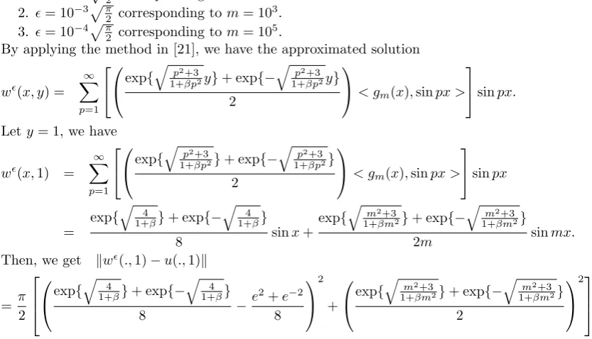
2 corresponding tom= 10 5.
By applying the method in [21], we have the approximated solution
w(x, y) = ∞ X p=1
exp{q1+p2βp+32y}+ exp{− q
p2+3
1+βp2y} 2
< gm(x),sinpx >
sinpx.
Lety= 1, we have
w(x,1) = ∞ X p=1
exp{q1+p2+3βp2}+ exp{− q
p2+3
1+βp2} 2
< gm(x),sinpx >
sinpx
=
exp{q 4
1+β}+ exp{−
q
4 1+β}
8 sinx+
exp{qm2+3
1+βm2}+ exp{− q
m2+3
1+βm2}
2m sinmx.
Then, we get kw(.,1)−u(.,1)k
= π 2
exp{q 4
1+β}+ exp{−
q
4 1+β}
8 −
e2+e−2
8 2 +
exp{qm2+3
1+βm2}+ exp{− q
m2+3
1+βm2} 2 2 .
Notice that if we choose β = and m such that β == pπ
2 1
m then kw
(.,1)− u(.,1)k does not converges to zero. Thus, by choose some different values, we have the table numerical test as follows
1. = 10−2pπ
2 corresponding tom= 10 20.
2. = 10−3pπ
2 corresponding tom= 10 20.
3. = 10−4pπ
Table 2. The error of the method in [7].
v a=kv(.,1)−u(.,1)k 1= 10−2pπ2 0.929362864692100 sin(x) 0.0140196447310024
+3.786855438.10−17sin(1020x)
2= 10−3pπ2 0.939414328021399 sin(x) 0.00142200363973089
+9.255956190.10−9sin(1020x)
3= 10−4
pπ
2 0.940435300951564 sin(x) 0.000142403832491343
+3.104968144×10⁻¹²sin(1020x)
From Table 1 and Table 2, we note that the results become less accurate when the error level increases which indicates that the method is useful. In table 2, for m large, we find that the numerical results become less accurate. To obtain bet-ter results, we should choose m which is suitable. However, ifm is not large, the method is not effective.
Looking at Tables 1,2 a comparison between the two methods, we can see the error results of in Table 1 are smaller than the errors in Tables 2. In the same parameter regularization, the error is Table 1 converges to zero more quickly many times than the Table 2 . This shows that our approach has a nice regularizing effect and give a better approximation with comparison to the many previous results, such as [2, 4, 5, 9, 21]. In addition, writing down (29) implies you can evaluate the inner product< gm(x),sin(mx)>, which is not easy ifgmis random noisy perturbation ofg.
6. Conclusion
In this paper, we use a new regularization method to solve the Cauchy problem for the modified Helmholtz equation in a rectangular domain. The convergence results have been presented for the cases of 0 < y < 1 and y = 1 under some different a-priori bound assumptions for the exact solution. Finally, the numerical results show that the proposed method works effectively.
Acknowledgments. The authors would like to thank the anonymous referee for his/her comments that helped us improve this article.
References
[1] L. Bourgeois, A mixed formulation of quasi-reversibility to solve the Cauchy problem for Laplace equation, Inverse Problems21(3) (2005), 1087–104.
[2] H.W. Cheng, J.F. Huang, T.J. Leiterman, An adaptive fast solver for the modified Helmholtz equation in two dimensions, J. Comput. Phys.211(2) (2006), 616–637 .
[3] J. Cheng, M. Yamamoto, Unique continuation on a line for harmonic functions, Inverse Problems,14, (1998) 869–882.
[4] L. Elden, Approximations for a Cauchy problem for the heat equation, Inverse Problems3
(2) (1987) 263–273.
[5] L. Elden, Solving an inverse heat conduction problem by a method of lines, J. Heat Transfer Trans. ASME119(3) (1997) 406–412.
[6] L. Elden, F. Berntsson, T. Regiska,Wavelet and Fourier methods for solving the sideways heat equation, SIAM J. Sci. Comput.21(6) (2000), 2187–2205 (electronic).
[8] J. Hadamard, Lectures on Cauchy Problem in Linear Partial Differential Equations, Dover Publications, New York, 1953.
[9] D. N. Hao and D. Lesnic , The Cauchy for Laplace equation via the conjugate gradient method, IMA Journal of Applied Mathematics,65(2000), 199–217.
[10] Y. C. Hon and T.Wei , Backus-Gilbert algorithm for the Cauchy problem of laplace equation, Inverse Problems,17: 261-271(2001).
[11] Y.C. Hon, T.Wei, Solving Cauchy problems of elliptic equations by the method of fundamental solutions, in: Boundary Elements XXVII, WIT Trans. Model. Simul. vol.39, WIT Press, Southampton, 2005, pp. 57–65.
[12] V. Isakov, Inverse problems for partial differential equations, in: Applied Mathematical Sci-ences, vol.127, Springer-Verlag, New York, 1998.
[13] A.H. Juffer, E.F.F. Botta, B.A.M.V. Keulen, A.V.D. Ploeg, H.J.C. Berendsen, The electric potential of a macromolecule in a solvent: a fundamental approach, J. Comput. Phys.97(1) (1991) 144–171.
[14] M.V. Klibanov, F. Santosa, A computational quasi-reversibility method for Cauchy problems for Laplace equation, SIAM J. Appl. Math.51(6) (1991) 1653–1675.
[15] M.V. Klibanov, A. Timonov, Carleman estimates for coefficient inverse problems and numer-ical applications, in: Inverse and Ill-posed Problems Series, VSP, Utrecht, 2004.
[16] X. Li, On solving boundary value problems of modified Helmholtz equations by plane wave functions, J. Comput. Appl. Math.195(1) (2006) 66–82.
[17] J. Liang, S. Subramaniam, Computation of molecular electrostatics with boundary element methods, Biophys. J.73(4) (1997) 1830–1841.
[18] L. Marin, D. Lesnic, The method of fundamental solutions for the Cauchy problem associated with two-dimensional Helmholtz-type equations, Comput. Struct.83(4) (2005) 267–278. [19] L. Marin, L. Elliott, P.J. Heggs, D.B. Ingham, D. Lesnic, X. Wen, Conjugate
gradient-boundary element solution to the Cauchy problem for Helmholtz-type equations, Comput. Mech.31(3) (2003) 367–377.
[20] L. Marin, L. Elliott, P. Heggs, D. Ingham, D. Lesnic, X.Wen, BEM solution for the Cauchy problem associated with Helmholtz-type equations by the Landweber method, Eng. Anal. Boundary Elem.28(9) (2004) 1025–1034.
[21] Hai-Hua Qin, Ting Wei, Quasi-reversibility and truncation methods to solve a Cauchy prob-lem for the modified Helmholtz equation, Mathematics and Computers in Simulation, Vol.80, Issue 2, 352–366.
[22] Z. Qian, C.L. Fu, Z.P. Li, Two regularization methods for a Cauchy problem for the Laplace equation, J. Math. Anal. Appl.338(1) (2008) 479–489.
[23] Z. Qian, C.-L. Fu, X.-T. Xiong, Fourth-order modified method for the Cauchy problem for the Laplace equation, J. Comput. Appl. Math.192(2) (2006) 205–218.
[24] H. J. Reinhardt, H. Han, D. N. H‘ao, Stability and regularization of a discrete approximation to the Cauchy problem of Laplace equation, SIAM J. Numer. Anal.,36, (1999), 890–905. [25] T. Regiska, K. Regiski, Approximate solution of a Cauchy problem for the Helmholtz
equa-tion, Inverse Problems22(3) (2006) 975–989.
[26] W.B. Russell, D.A. Sville, W.R. Schowalter, Colloidal Dispersions, Cambridge University Press, Cambridge, 1991.
[27] A. Tikhonov, V. Arsenin, Solutions of Ill-posed Problems, V.H. Winston Sons, Washington, DC, John Wiley Sons, New York, 1977.
[28] C.F. Weber, Analysis and solution of the ill-posed inverse heat conduction problem, Int. J. Heat Mass Transf.24(11) (1981) 1783–1792.
[29] T.Wei, Y. Hon, L. Ling, Method of fundamental solutions with regularization techniques for Cauchy problems of elliptic operators, Eng. Anal.Boundary Elem.31(4) (2007) 373–385. [30] A. Yoneta, M. Tsuchimoto, T. Honma, Analysis of axisymmetric modified Helmholtz equation
by using boundary element method, IEEE Trans. Magn.26(2) (1990) 1015–1018.
T. Huy Nguyen , Division of Applied Mathematics, Ton Duc Thang University, Nguyen Huu Tho Street, District 7, Hochiminh City, Vietnam.
Phan Van Tri, Division of Applied Mathematics, Ton Duc Thang University, Nguyen Huu Tho Street, District 7, Hochiminh City, Vietnam.
E-mail address:[email protected]
Ho Vu, Division of Applied Mathematics, Ton Duc Thang University, Nguyen Huu Tho Street, District 7, Hochiminh City, Vietnam.
E-mail address:[email protected]
Ngo Van Hoa, Division of Applied Mathematics, Ton Duc Thang University, Nguyen Huu Tho Street, District 7, Hochiminh City, Vietnam.
![Table 2. The error of the method in [7].](https://thumb-us.123doks.com/thumbv2/123dok_us/8761709.1752283/10.595.138.475.137.227/table-error-method.webp)
