Anticipatory Routing for Highly Mobile Endpoints
Fabrice Tchakountio
BBN Technologies
Internetwork Research Department
Cambridge, MA 02138
[email protected]
Ram Ramanathan
BBN Technologies
Internetwork Research Department
Cambridge, MA 02138
[email protected]
Abstract
We consider the problem of routing to endpoints with very high “effective” mobility, i.e, when the period between changes in an endpoint’s location is comparable to the time it takes for the location tracking mechanism to converge. This could happen due to increased endpoint speed, increased control message latency, or decreased cell size. When this happens, conventional location tracking approaches fail – by the time such mechanisms converge, the endpoint has already moved to a new location, and we say the “reactive limit” has been reached. When mobility exceeds the reactive limit, pre-diction techniques are required for network control.
We describe “anticipatory routing”, a mechanism that uses a limited history of past movement of the endpoint to predict its future locations. In particular, we use linear re-gression to predict future locations and affiliation/departure times of the endpoint. Using a simulation model of a multi-hop wireless network, we study the performance of anticipa-tory routing. Our results indicate that above a certain mobil-ity threshold, anticipatory routing significantly outperforms conventional location tracking mechanisms. Its magnitude of improvement increases with higher mobility – in particular, its rate of throughput degradation with speed is 56% better.
1. Introduction
All mobile networks employ some control mechanism to route packets to mobile endpoints (hosts). This typically con-sists of a location tracking mechanism to determine the net-work attachment point of the mobile endpoint, and a routing mechanism to forward the packets there [1]. The efficacy of such mobility management mechanisms depends on the rela-tionship between two factors: the frequency of “state” change (e.g. change in network attachment point or location) for an endpoint, and the time it takes for the control mechanism to converge to reflect the new state. The vast body of work on control mechanisms has focused on situations when the fre-quency of state changes is low, so that the control mechanism
has ample time to react and converge to the new state. The question we address here is: What if the frequency of changes is high, and in the extreme, so high that by the time the con-trol mechanism converges, the endpoint has already moved to a new location?
Why is this question important? The evolution of archi-tectures for mobile networks is governed by some key con-straints: the need for high data rates (e.g: support of unteth-ered multimedia communications), the scarcity of commu-nications spectrum, and the need to conserve battery, and hence transmission power. Consequently, network architec-tures are evolving towards short links. Smaller cells and shorter links imply an increase in frequency of cell changes. On the other hand, network infrastructures are not only in-creasing in size, but also evolving toward a larger wireless component (e.g. [2]). This results in an increase in the la-tency of control messages and therefore an increase in the convergence time of the control mechanism. Increasing fre-quency of network state changes and increasing convergence time of control procedures may well push network dynamics into the realm where control mechanisms are constantly out-paced by the endpoint’s cell changes. Note that it is not the absolute speed of an endpoint but its relation to the cell size and convergence time of the mobility management mecha-nism that actually matters.
We define effective mobility as the ratio between the con-vergence time and the cell presence time (inverse of the cell change frequency). When the effective mobility exceeds the value of 1, we say that the reactive limit has been reached – that is, the (average) convergence time exceeds the (aver-age) cell presence time.
Thus, for mobility regimes that take the system beyond the reactive limit, a predictive mechanism that shifts the tar-get location to an anticipated location based on current infor-mation is required. This paper focuses on anticipatory
rout-ing as the predictive mechanism to address this problem.
An overview of the forthcoming sections is as follows. Sections 2, 3 provide the context for our work. Section 4 presents anticipatory routing followed by an experimental study in section 5. Section 6 concludes this paper.
2. Related Work
One technique for addressing very high effective mobil-ity is spray routing [3]. Spray routing multicasts data traffic in the vicinity of the last “known” location. Although it im-proves the throughput, spray routing has several shortcom-ings. First, it is not effective beyond a certain effective mo-bility. Second, it generates a significant overhead in duplicate packets with increased mobility, causing higher end-to-end delays. This makes spray routing hardly practical in current and next generations of cellular systems, where channel ac-cess is very limited.
A relatively small amount of previous research has investi-gated ideas similar to anticipatory routing in that “prediction of future locations based on location history information” is used. In [5], the authors present Trajectory-Based Forward-ing (TBF), a method to forward packets in a dense ad-hoc network based on a predefined trajectory curve. TBF has sev-eral benefits. It addresses scalability issues such as mobil-ity rate and network size. It also provides a common frame-work for many services such as broadcast, multicast, and so on. In [6], the authors propose a Robust Extended Kalman Filter (REKF) as a state estimator in predicting the mobile user’s expected trajectory. In particular they focus on an al-gorithm for mobility estimation for a network in which base stations and user terminals are mobile. In [7], the author pro-poses that a mobile terminal’s location can be derived from its quasi-deterministic mobility behavior and can be repre-sented as a set of movements in a user profile. [8] proposes an enhancement to [7] based on a pattern matching/recognition-based mobile motion prediction (MMP).
Our work differs from existing work in several respects. A fundamental difference is in the reactability of the loca-tion tracking and routing mechanism - while previous works take the timely convergence of the respective control mecha-nism as a given, our work is motivated precisely when this is not true. In particular, we consider different regions of opera-tion of the system depending on the effective mobility of the endpoint, and we apply a prediction technique when the ef-fective mobility of the endpoint becomes high.
3. Network Architecture
In order to study anticipatory routing in a reasonable man-ner, we need to provide a context for its operation. Specifi-cally, we need to have a model for how the network “works” and how the information used by anticipatory routing will be obtained. Further, such an architecture and mechanism must be fairly generic rather than tied to a particular standard.
This section discusses a network architecture and location tracking mechanism as the context for anticipatory routing. It is not our intent to propose new network architectures or lo-cation tracking mechanisms. Rather, we merely want to de-velop a model that can capture the way emerging networks work.
Our network consists of two kinds of nodes: switches and endpoints. Switches perform routing functions1and end-points can be sources of or destinations for packets. End-points have one-hop wireless link to some switch, and the switches form a mesh network. The traffic is stream-oriented - e.g. packetized voice, video, as envisaged in 3G PCS sys-tems. This captures both cell-based networks (e.g. GSM) as well as broadband wireless mesh networks (e.g. [2]). For in-stance, in a cell-based network a switch corresponds to a base station, and some switches are mobile switching centers. An endpoint corresponds to a mobile host.
3.1. Affiliation/ Handoff process
An endpoint selects a one-hop-away switch for commu-nication to and from other endpoints. Such an endpoint and switch are said to be affiliated with one another. The region in which endpoints can affiliate with a given switch S is de-fined as the cell S. The location of an endpoint is the switch with which it is affiliated. Due to switch or endpoint mobil-ity, an endpoint might change its location or cell. This is re-ferred to as handoff. In our system, an endpoint initiates a handoff if and only if the received signal quality from the af-filiated switch falls belowq/α, whereqis the minimum qual-ity for successful reception, andαis the coefficient that con-trols the signal quality threshold,0 < α < 1. The lowerα is, the higher the threshold value becomes. It then affiliates with the switch from which it receives the best signal qual-ityq0, ifq0is better thanq/α. Note that the affiliation is done proactively, that is, without waiting for the signal quality to be totally unacceptable. Thus, an endpoint is able to still com-municate with the previously affiliated switch while the af-filiation with the new switch, and location management (de-scribed in the next section) processes are in progress. This ”overlap” time increases with decreasingαbut so does the frequency of handoffs. Our handoff process reflects current practice in many PCS systems and falls into the class of ”strong early” techniques [9].
3.2. Location Tracking
In simplest terms, location tracking answers the question: given an endpoint, which cell is it in? Over the past decade, a large number of location tracking schemes have been pro-posed [1, 10]. In our case, we are faced with the problem
of selecting a solution for the unique combination of very high mobility and stream-oriented traffic. In particular, our focus is on how best to handle multiple handoffs within the span of one session. Thus, fast convergence time is of utmost importance. Clearly, paging is not appropriate here. Nor is the Mobile-IP [11] method of always going through a home agent (or the conceptually equivalent approach of HLRs and VLRs [1]), since the triangular routing property may induce large end-to-end packet delays. Not finding an existing tech-nique appropriate for our purposes, we have designed a rudi-mentary location tracking scheme that borrows ideas from several previous approaches, as described below.
A configured number ofKswitches act as location man-agers (LM). Each LM maintains a location database. An endpoint D is mapped into one location manager L using a simple hashing function. That is, the switch L will always store the location information for endpoint D, irrespective of the location ofD. The location manager ofDis denoted LM(D). A switch may be a location manager for multiple endpoints. Endpoints update their location managers when their affiliation changes using a Location Update. When a source of trafficS wishes to set up a session with a desti-nationD,Ssends a Location Subscribe message toLM(D). With this message,Sasks for the location ofDand for fresh updates wheneverD’s location changes. Since the sourceS may itself be mobile, LM(D) in turn initiates a Location Subscription toLM(S). After this step, any change inD’s (resp.S’s) location will be automatically conveyed toS(resp. LM(D)) byLM(D)(resp.LM(S)) using a Location Infor-mation message. This happens untilS, upon session termi-nation, sends a Location Unsubscription message toLM(D) andLM(D) initiates in turn a Location Unsubscription to LM(S). An example is shown in figure 1.
How sensitive are our results to the choice of the location tracking mechanism? We believe that it would change the ex-act values of transition points, but the results will largely fol-low the same pattern. This is because in all efficient loca-tion tracking mechanisms, there is a lag between when a state change happens and when the system knows about it. It is this lag that is largely responsible for the system dynamics stud-ied in this paper. Different location tracking mechanisms will give rise to different lags and shift the effective mobilities at which transitions happen, but they will happen nonetheless. In other words, the choice of the location tracking mecha-nism affects the quantitative results but not the qualitative.
3.3. Routing protocol
Our system uses a flat link-state routing mechanism [13] between the switches. Event driven and periodic updates are flooded throughout the network and routes are generated us-ing Dijsktra’s shortest path algorithm. Hop-by-hop packet forwarding is used. For further details on this protocol, please refer [13].
3.Unsubscribe
D
S
LM(D)
0. Update
1. Subscribe
2. Info
Figure 1. Messages comprising our location tracking mechanism.
4. Anticipatory Routing
Anticipatory routing predicts where a session’s destina-tion endpoint will be at a particular time and forwards traffic directly to the predicted location. We consider Anticipatory routing when apriori information about the endpoint’s move-ments is not available2. We however exploit the fact that in a real life situation, endpoints with high velocity are more likely to move in a straight line for a while. While this is not an explicit assumption, it is implicit in the mobility model we use, and is a factor in the predictive ability of our algo-rithm.
4.1. Algorithm Description
To support anticipatory routing, the basic location tracking mechanism that we proposed in section 3.2 is modified. Link state update (LSU), location update (LU) and location infor-mation (LI) messages are augmented with additional fields as explained below:
LSU is augmented with the physical location (position) in-formation of its initiator. In our system all switches are GPS-enabled. LU is augmented with the timetak that the
affili-ation happened as well as the physical locaffili-ation informaffili-ation XkofD’s switch.Dlearns aboutXkfrom signaling message
exchanges with its switch. In our system we neglect physical location errors.
Let Ak denote the switch identifier of D, and Hk =
(Ak, tk(a), Xk)the new information added into the LU. Upon
affiliation with Ak, D updates LM(D) with LU reporting
Hk.LM(D)- based on a limited history of size L of D’s
movementHk = (Hk−L+1, .., Hk)- predicts a set ofW
fu-ture locationsA˜k+1= ( ˜Ak+1, ..,A˜k+W)along with a set of
D ~
A
A
~
4 5
A 3 A 2
A 1 Actual D’s trajectory
Estimated trajectory (using linear regression)
Figure 2. Illustration of estimated against ac-tual trajectory.
Waffiliation timesT˜k(a)= (˜tk(a+1) , ..,˜t(ka+)W)andW+1 depar-ture timesT˜k(d)= (˜t(kd), ..,˜t(kd+)W). Next,LM(D)adds the set of predicted information( ˜Ak+1,T˜
(a)
k ,T˜
(d)
k ),Ak,tk(a)into
the LI and conveys this to source S. The following lines de-scribe the three basic steps necessary to predict future loca-tions and affiliation-departure times ofD.
4.1.1. Estimation of endpoint’s trajectory Estimating the
trajectory of the endpoint is accomplished using a modified
linear regression, where changes inD’s linear direction are detected.
The algorithm works as follows.
Say the set of switch positions for cells crossed by D are Xk−L+1, ..., Xk; whereXk = (xk, yk)are position
coordi-nates in the two dimentional space;Lis the location history size.
LM(D)first picks a set of two and three latest positions (Xk−1, Xk)and(Xk−2, Xk−1, Xk). For each of these sets,
it computes two linear regression equations (m1, h1) and
(m2, h2). The resulting slopesm1andm2are used to
deter-mine trajectory directionsθ1 andθ2. If|θ1−θ2| > θthresh
then we say thatDhas changed its direction. Consequently, the trajectory equation is(m1, h1), which representsD’s
tra-jectory after the ”turn”. Otherwise, no turn has been observed andLM(D)does the same processing using the last three and four positions. This process repeats until a turn is de-tected or the current largest set matches the history sizeL, whichever occurs first. Thus, a linear equation(m, h)is re-turned. An illustration ofD’s estimated trajectory is depicted in figure 2.
Why linear regression? In general, endpoints are more likely to move in straight lines for a while at high mobil-ity. It makes sense therefore to estimate the linear trajectory of that endpoint. Linear regression fits well among possi-ble techniques since it relies on the least-square error
the-ory. This means that the estimated linear trajectory is likely to be close enough to positions actually traversed by the end-point.
4.1.2. Estimation of endpoint’s direction An endpoint’s
direction is derived from the slopemof the trajectory equa-tion, the current positionXkand last position in historyXk−t
where a change in direction (if any) is observed. This process is necessary to select future locations.
4.1.3. Prediction of future location, affiliation/departure
time From an estimate of D’s trajectory, position of D’s
last known switch position Xk and network topology
in-formation, LM(D) derives D’s future location. Given (m, h) the estimate of D’s trajectory equation and posi-tionsX˜k+1, ..X˜k+W, one can deriveDkthe average distance
to cross a cellAk (see [12], section K.25). If we
approxi-mateV,D’s average speed, as
V = 1 L−1
L−1
X
i=0
−−−−−−−→
||XiXi−1||
|Ti−Ti−1|
(1)
The duration to cross the cellDk/V can be used to form the
departure time from the current cell
˜
t(kd)=tk(a)+Dk/V
Wheretk(a) represents the known affiliation time to the
current cell.
LetXk(d)(resp.X˜
(a)
k+1) the rightmost (resp. leftmost)
po-sition intersecting the trajectory and cell Ak (resp. A˜k+1)
(see [12], section K.25). Say each cell has a radius ofR me-ters, then the affiliation time toA˜k+1is
˜ t(ka+1) =
˜
t(kd), Xk
(d)X˜(a)
k+1
≤2R;
˜ t(kd)+
Xk
(d)X˜(a)
k+1
V , otherwise.
Subsequent times t˜(kd+1) and ˜t(ka+2) can be derived using the same process above.
Data Forwarding is done as follows. Recall that switches only are GPS-capable in our system. Thus, a switch that is responsible for a given source-nodeS sets a timestamp into packets originated byS. Packet end-end delays are derived from those timestamps. Upon data transmission by sourceS, S’s switch selects the appropriate destination cell based on the current time, the estimated end-to-end delay and the latest prediction information, and forwards the packet to the desti-nation switch. The destidesti-nation switch may or may not be a predicted. Switches other than the source do not change their regular behavior.
4.2. Anticipatory Routing Limit
of the effective mobility (see [3], section 5). The first is the
re-actable state, where all packets always reach the destination.
The throughput in this case is always 100%. This state often occurs when the destination is static or has very low mobil-ity. The second is the late-reactable state, where some of the packets reach the destination and some do not. The through-put in this case is between 0 and 100%. The third is the
un-reactable state, where no packet reach the destination. The
throughput in this case is always 0. This state represents the reactive limit of the system.
A question about anticipatory routing is: what is the un-reactable state when anticipatory routing is in use? In other words, what is the speed limit beyond which the throughput is always 0? We address this question below.
Say source S communicates with destination D. Say S sends one packet toD. WhenS’s switch receives the packet att0, it selects the appropriate location based on the current
prediction information and an estimate of the network delay d. For instance, a data packet will be sent to the k-th loca-tionA˜kif
˜
t(ka)≤t0+d≤˜t (d)
k (2)
We can reasonably assume that anticipatory routing is out-paced by D’s mobility when
t0+d >˜t (d)
k+W (3)
WhereWrepresents the number of predictions.
In the context of cellular networks with overlapping cells ˜
t(ka+1) = ˜t(kd). IfTcell(k), representing the cell presence time
inAk, is approximated by its mean valueTcell, then the
de-parture time from the last predicted cell is given by
˜
t(kd+)W = t˜(ka+)W +Tcell
= ˜t(kd+)W−1+Tcell
= ˜t(ka+)W−1+ 2Tcell
= ˜t(kd+)W−2+ 2Tcell
= ˜t(ka+)W−2+ 3Tcell
yielding the final expression
˜
t(kd+)W =tk(a)+ (W+ 1)Tcell (4)
From the analysis in [3], section 5.1
d=N0H = N−1
H (5)
From the analysis in [3], section 5.1, timet0is such that
t0 > tk(a)+Tupdate+Tinf o+H (6)
> tk(a)+ (2N+ 1)H; (7)
Where N represents the average number of hops between sourceS and cellhead ofD, andH represents the average per-hop delay.
From equations (3), (4), (5), the system enters the unre-actable state if
t0+ N−1
H > tk(a)+ (W+ 1)Tcell (8)
By substituting the lower bound oft0in equation (7), the
system enters the unreactable state when
3N H >(W+ 1)Tcell (9)
Tcellis expressed ([3]) by
Tcell=
4pA/π πV
From equation (9) andTcellexpression, the anticipatory
routing limit expression is given by
V > 4(W+ 1) p
A/π
3N H (10)
The reactive limit of a conventional tracking system (as de-scribed in [3]) is given by
V >4 p
A/π
(3N H)
Therefore, the antipatory limit in equation (10) can be ex-pressed as a function of the reactive limit as follows:
Vanticipatorylimit= (W + 1)Vreactivelimit
This means that anticipatory limit increases proportionally to the size of prediction information. The anticipatory system results in a reactive system when no prediction is done.
5. Experimental Environment
After careful consideration of several simulation environ-ments including OPNET, NS-2, and PARSEC, we decided to build our simulations from scratch using C++. The main reason for this is that we wanted to independently control the tradeoff between fidelity (detail) and performance at each layer of the stack, and none of the above mentioned simula-tors provided what we wanted.
An instance of a multihop mobile wireless network is gen-erated by placing a set of S switches and E endpoints in an L meters x L meters square area. Switches are distributed in a Manhattan grid form. Each switch (resp. endpoint) is given a communication range ofRs(resp.Re) meters. Free-space
propagation is assumed with threshold cut-off. That is, two nodes can communicate with each other if and only if their Euclidean distance is less or equal than a threshold, in partic-ular,Rsbetween switches andRebetween an endpoint and
a switch. The system is assumed free of losses due to propa-gation effects such as noise, fading, etc3. Packet losses may
only occur when a packet gets to the destined switch but the destination endpoint is not affiliated with it.
Each cell has a communication range ofRe. We assume
free-space propagation and therefore use distances in lieu of signal strengths (see section 3.1) to effect handoffs. The mo-bility model is an Extended Random Walk (ERW) model (see [14]). Each node moves in certain direction, during a pe-riod of time of epochifor a constant duration and with a con-stant speed, then it picks another direction and moves in that direction for another constant duration and constant speed, and so on. Speed, direction, and epoch length are uncorre-lated. Mobility is uncorrelated among the nodes of the net-work.
Each node’s direction is uniformly distributed over the space of discrete values – 0, 45, 90, 135, 180, 225, 270, 315, 360 degrees. We use a ”spherical” or ”wraparound” model where nodes reappear from the opposite side. There are no boundaries. The queueing delay at each node as well as the transmission delay is modeled. Each packet is de-layed by a time roughly proportional to the congestion in the neighborhood of the forwarding node. Our traffic model is stream-oriented: A source (endpoint) picks one destina-tion(endpoint) and sends data packets using an on/off model, each on phase corresponding to a session. Packets within a session are generated by Bernouilli trials with parameter (1−1/e). Unless otherwise mentioned, we use the following parameters for our network: number of switchesS = 100; number of active endpointsE = 40(20 traffic node pairs); density ND = 100 node/sq km; cell radiusRe= 80m; packet transmission time = 100 ms; and α = 0.9. These parame-ters reflect future trends (such as third generation cellular net-works), including an increased reliability on wireless relays to extend the reach - this is the reason for the somewhat large number on the per-hop delay. In addition to these, L=5, W=2,
θthresh(see section 4.1)= π/4. There are 3 epochs per run
and each epoch lasts 100 seconds. For all curves, each point is an average of 5 experiments.
5.1. Analysis
We study the dependence of anticipatory routing as a func-tion of the endpoint’s speed. Metrics of particular interest are:
• Throughput. The fraction of packets sent by any source
that was successfully received at the destination.
• Anticipated Fraction. The fraction of data packets sent
by any source to locations that are predicted, rather than known in advance.
• Delay. End-End delay for successful data packets.
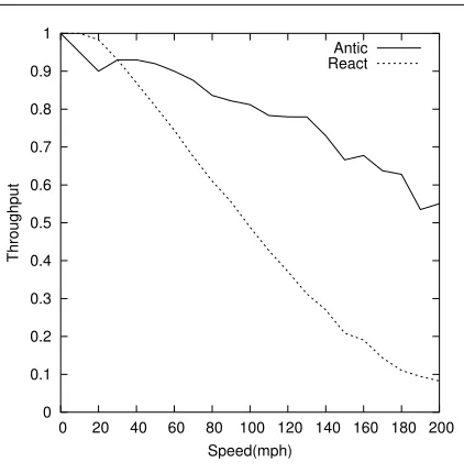
One can observe that anticipatory routing does worse at very low speeds compared to a pure reactive mechanism (sec-tion 3.2) as shown in figure 3. This is caused by inaccuracies in speed estimation derived in equation 1. These inaccuracies might lead, for instance, to shorter estimated cell-presence
0 0.1 0.2 0.3 0.4 0.5 0.6 0.7 0.8 0.9 1
0 20 40 60 80 100 120 140 160 180 200
Throughput
Speed(mph)
Antic React
Figure 3. Average throughput for anticipatory routing and traditional routing.
time. Consequently, data packets intended for known loca-tions get erroneously forwarded to predicted localoca-tions. At about 30 mph, anticipatory routing and reactive routing re-turn a throughput of 92%. Such levels of throughput degra-dation (packet loss) challenges TCP performance. However, at higher speeds, anticipatory routing performs better and of-fers a throughput above 50% for all cases considered. Conse-quently, we expect that loss-tolerant applications (with degra-dation in quality), such as those used for situation awareness update (video/imagery) can achieve a better quality with an-ticipatory routing. For non-loss tolerant applications, mecha-nisms to enhance reliability and performance under loss have been proposed [15, 16, 17]; evaluating their applicability to anticipatory routing is a subject of future research.
For speeds > 30 mph, anticipatory routing keeps the degradation low compared to the reactive scheme. Within 30-200 mph4 range, slope of anticipatory routing and reactive curves are respectively−0.002231 mph−1 and−0.004987 mph−1, resulting therefore in 56% lesser (better) through-put degradation with anticipatory routing. Furthermore, the anticipated fraction (figure 4) increases steadily because a higher speed increases the likelihood of packets to be sent to a predicted location. With increasing speeds, destination endpoints are less likely to be at their known locations and the predictive algorithm detects where the right locations are.
0 0.1 0.2 0.3 0.4 0.5 0.6 0.7 0.8 0.9 1
0 20 40 60 80 100 120 140 160 180 200
Anticipated Fraction
Speed(mph) Antic
Figure 4. Anticipated Fraction for anticipatory routing.
Also, one can notice a significant rise in end-end delay with the speed for either mechanism (figure 5). This hap-pens because control messages increase with the frequency of affiliations, causing higher channel access delays. Given the high per-hop delay, packets that reach their targets are likely to have encountered high delays along the path. However, in the reactive case, this effect is somewhat reduced above 180 mph. Indeed, less than 1% of packets reach their destination and the successful packets have likely encountered lower net-work delays. Unlike the reactive scheme, anticipatory routing works effectively regardless of the congestion in the network. Also, high speeds give rise to very high delays (figure 5) – around 2.5 seconds on average. These delays are primar-ily due to queueing delays, which in turn are a consequence of the relatively low data rate used in our simulation, namely about 200 kbps. We used this as a conservative estimate of the data rates that a metropolitan area wireless ad hoc net-work might offer. With time, we should see these rates in-crease and so the delay should drop to reasonable numbers.
6. Conclusion
We have presented a novel mechanism that addresses the problem of routing to endpoints with very high ”effective” mobility. Anticipatory routing estimates future locations of an endpoint based on past trajectory information and for-wards session traffic directly to the predicted location. In par-ticular, linear regression is employed. We have derived an expression for the limits of anticipatory routing. Our exper-iments show that anticipatory routing improves the perfor-mance of routing at high mobility (by 56%) compared to
0.25 0.5 0.75 1 1.25 1.5 1.75 2 2.25 2.5 2.75 3 3.25 3.5
0 20 40 60 80 100 120 140 160 180 200
Delay(sec)
Speed(mph)
Antic React
Figure 5. Average end-end delay for anticipa-tory routing and reactive routing.
the reactive scheme. In practice anticipatory routing could augment a mechanism such as Mobile IP [11] where home
agents would keep an history of endpoint’s movements and
would derive their predicted location upon reception of a data packet. Tunnel headers of those packets would include an an-ticipated care-of-address at high mobility.
Our work should be useful to wireless network design-ers seeking to implement routing solutions that meet perfor-mance demands in networks with highly mobile terminals.
Acknowledgement
We thank Rajesh Krishnan (BBN Technologies) for his helpful feedback on this paper.
References
[1] R. Ramanathan and M. Steenstrup, “A survey of routing tech-niques for mobile communication networks”, Mobile Networks and Applications 1(1996), 89-104.
[2] Mesh Networks Inc., http://www.meshnetworks.com
[3] F. Tchakountio and R. Ramanathan, “Tracking Highly Mobile Endpoints”, In proc. of ACM Workshop on Wireless Mobile Multimedia (WowMom), July 2001, Rome, Italy.
[4] A. Bhattacharya and S.K. Das, “Lezi-update: An information theoretic approach to track mobile users in PCS networks”, Proc. of Mobicom 99, August 1999.
[6] P. Pathirana, A.V. Savkin, S. Jha, “Mobility Modeling and Tra-jectory Prediction for Cellular Networks with Mobile Base Sta-tions”, Proc. of MobiHoc, June 2003.
[7] S. Tabane. “An alternative strategy for location tracking”, IEEE JSAC, June 1995.
[8] G. Liu and G. Maguire. “A predictive mobility management scheme for supporting wireless mobile computing ”, In proc. IEEE Int. Conf. Universal Personal Communication, 1995. [9] T. Camp, J. Lusth, J. Matocha and C. Perkins, “Reduced Cell
Switching in a Mobile Computing Environment”, Proc. ACM Mobicom 2000.
[10] R. Ramanathan and M. Steenstrup, “Hierarchically-organized; multihop mobile wireless networks for quality-of-service sup-port”, Mobile Networks and Applications, vol. 3, no. 1, pp. 101-119,1998.
[11] Mobile IP, Internet Request for Comments (RFC 2002) [12] F. Tchakountio, R. Ramanathan, “Routing to Highly
Mo-bile Endpoints: A Technical and Experimental Study of Lim-its and Solutions ”, BBN tech. report 1280, December 2000, http://www.ir.bbn.com/projects/highmob/highmob-index.html. [13] A.S. Tanenbaum, “Computer Networks”, Prentice-Hall 1996 [14] A.B McDonald and T.F. Znati, “A Mobility-Based Framework
for Adaptive Clustering in Wireless Ad Hoc Networks”, IEEE JSAC, Aug.1999, pp 476-1486.
[15] A.J McAuley, “Reliable Broadband Communication Using a Burst Erasure Code”, In Proceedings of ACM SIGCOMM’90, Philadelphia, PA, USA, September 1990.
[16] M.A Jolfaei, B. Heinrichs, and M.R Nazeman, “Improved TCP Error Control for Heterogeneous WANs”, In Proceedings of IEEE National Telesystems Conference, San Diego, CA, USA, May 1994.