Massive Collaborative Wireless Sensor Network Structure Based on Cloud Computing

Massive Collaborative Wireless Sensor Network

Structure Based on Cloud Computing

https://doi.org/10.3991/ijoe.v14i11.9499

Qiong Ren

Jianghan University, Wuhan, China [email protected]

Abstract—To explore the wireless sensor network (WSN) structure, the co-operative WSN architecture of mass data processing based on cloud computing is studied. The technology of WSN and cloud computing is deeply discussed. The system and node structure of WSN are studied by theoretical analysis method, and the performance of the WSN is studied by using the numerical simulation method. The mass data processing technology based on Map Reduce and its ap-plication in WSN are discussed. The numerical simulation method is used to ex-periment on the architecture of SVC4WSN and MD4LWSN. The relationship between the optimal network number and the node communication radius at dif-ferent node density is verified. Moreover, the energy and time delay Reduce path is compared with three protocols of LEACH, PEGASIS and PEDAP. The results show that the two Reduce paths have better performance in both network survival time and the total time slot of data acquisition.

Keywords—WSN; massive data processing; cloud computing

1

Introduction

Since twenty-first Century, with the rapid popularization of automatic information generation equipment represented by sensors and intelligent recognition terminals, peo-ple can accurately perceive the data of the physical world in real time. As a new com-ponent of information technology, Internet of Things (IoT) has been widely concerned by many countries all over the world. The United States first regards the IoT as the direction of national strategic development. In 2009, International Business Machine Company put forward the strategy of "intelligent earth". In the same year, the Chinese government established the central goal of building a "perceived China" based on the IoT. According to the Forrester of the authoritative advisory body, by 2020, the world's interconnected business will reach 30:1 compared to the human communication busi-ness; by 2035, the wireless sensor network (WSN) terminal of China will reach hun-dreds of billions; and by 2050, the sensor will be ubiquitous in life and this is the scale effect of intelligent devices in IoT.

is still the Internet, and it is the network extended on the basis of the Internet; and the second is that its user end is extended to information exchange and communication between any object. At present, the mainstream definition of the IoT is proposed by the International Telecommunication Union in 2005. That is, the IoT is a network that con-nects any objects with the Internet for information exchange and communication to realize intelligent identification, location, tracking, monitoring and management of ob-jects through information sensing devices, such as ratio frequency identification, infra-red sensors, global positioning systems, and laser scanners. Compainfra-red to the traditional communication network or the Internet, the IoT will make every object in the world corresponding to a unique code, collect all kinds of signals through information com-munication and network technology, convert it into information flow, and combine it with the Internet, so as to form a new communication between people and objects and between objects and objects.

The IoT has become the next high point in the field of information technology. In the face of the coming large-scale application, the data processing and architecture of the IoT have become the focus of researches. The collaborative WSN architecture based on distributed mass data processing is proposed in the face of this urgent need. With the large-scale development of WSNs used by the perceptive layer in the IoT, the mas-sive data produced in this network need to be processed in time, and users expect to get more useful information from these data. Therefore, the research on massive data pro-cessing and collaborative WSN architecture has realistic and long-term significance.

2

Literature review

IoT is recognized as one of the key technologies for the third breakthroughs in the IT industry after the Internet and mobile communications technology. The first and foremost problem in the construction and application of IoT is how to deal with com-plex data. All the countries in the world have paid great attention to WSN and its ap-plications. The informational strategies such as the "intelligent earth" of the United States, the "u-Japan" of Japan, the "u-Korea" of Korea, the "European digital plan" of the EU and China's "perceived China" have developed rapidly. The common points of these informational strategies include the integration of various information technolo-gies, the breakthrough of Internet limitations, the access of objects to information net-work and the realization of object netnet-working. On the basis of the Internet populariza-tion, the information technology is applied to various fields, which has far-reaching influence on all aspects of the national economy and social life. The development of the future information industry extends and breaks through from the information net-work to the overall perception and intelligent application.

mathematical and physical basis of the technology needed to create a new information ecosystem, including one trillion nanoscale sensors and drives embedded in the large environment. The computer systems, software and services are connected through a variety of networks to exchange information between the analysis engine, the storage system and the end users.

The European Union (EU) has also carried out a lot of researches and applications in WSNs. On September 15, 2009, the EU issued the "road map of the strategic research on the IoT", and put forward the research field and research route of the EU's IoT for 2010-2020 years. This road map indicates that all "objects" in the vision of the IoT have a common feature, that is, "they can add sensors to interact with the environment where they are". The future technological development assumptions and research needs are put forward, among which sensors and WSNs are involved. The main research projects of WSNs in the EU include ARTEMIS (Advanced Research and Technology for Em-bedded Intelligence and Systems). ARTEMIS studied new multidisciplinary coordina-tion and control principles related to large-scale WSNs and actuator networks, includ-ing integrated control, computinclud-ing and communications (C3) strategy.

In the distributed large-scale WSN data processing, many scholars at home and abroad have put forward corresponding solutions.

Arora et al. (2016) proposed a data storage method based on distributed space and time similarity to improve the efficiency of data query in WSNs [1]. Zahurul et al. (2016) allocated the tasks of sensor nodes and put forward a kind of energy efficient data acquisition scheme with the aid of the correlation between space and time [2]. Olofsson et al. (2016) put forward the protocol for large scale WSN data collection to achieve the goal of maximizing the network lifetime by balancing the energy consump-tion of the whole network [3]. Wei et al. (2017) proposed a new storage and range query scheme in the data of the sensor network, reducing the message cost and obtaining the load balancing in the network [4]. Khasawneh et al. (2017) proposed the distributed data collection and distributed data aggregation algorithm in the large-scale heteroge-neous WSN under the generalized physical interference model [5]. Kumar and Kumar (2016) proposed a method based on distributed reinforcement learning routing in large-scale WSNs, and obtained satisfactory end-to-end delay and reliability [6]. Mai et al. (2016) put forward a distributed algorithm based on time and energy tradeoff for ag-gregation of large sensor network data [7].

the help of the elastic computing characteristics of Amazon EC2, the dynamic load requirements of the actual environmental application are met.

In general, the existing schemes cannot effectively solve the heterogeneity of the sensor network data, the support for the current mass data processing of the sensor net-work is not enough, and the data collected cannot be used very well. In view of this, the new WSN is combined with cloud computing architecture technology. It is mainly di-vided into two aspects: first, the cloud computing mass data processing technology is introduced to provide strong support for large-scale WSN data processing; second, for the large-scale WSN itself, the innovative architecture suitable for the massive data processing is put forward, which can better integrate with cloud computing.

3

Method

3.1 Sensor network structure Map

There are N nodes in the WSN, each node has a unique identifier number, which has nothing to do with the location of the node. Sink is deployed at the center of the region. The level number is allocated from 1, the most inner node (nearest to Sink) has the smallest level number, and the outermost node has the largest level number.

Define GCP for the global control frame sent by Sink node, which can be received by all nodes in the Sink managed area. In network initialization, Sink broadcasts a GCP message with the area radius R, which contains the total number of L of the ring net-work and the local communication reference radius rcom. The Sink node receives the

local control frames sent by the neighbor nodes within the distance rcom, and the sensor

nodes within the Sink node rcom will become the first layer of nodes, that is, the virtual

group head. Nodes will calculate the ring area limit value bk of the kth layer according

to the GCP message and Formula (1).

. (1)

The parameter represents the average distance from Sink node to the nodes in the k-1th layer, and its formula is shown in (2):

. (2)

In the data acquisition stage, the node of the k+1 layer will transfer the sensor data to the nodes in the kth layer, the node density ρ is usually a large value, and the sensor nodes are approximately uniform. Each node in the kth layer will receive approximately

data items from the k+1th layer node. is described in Formula (3).

î

í

ì

+

£

=

-

r

otherwise

b

k

b

,

0

,

0

b

2

1 -

-=

k

b

b

b

k

. (3)

When all nodes have identified their own layer, they will enter the stage of identify-ing their neighbor nodes. When the neighbor node receives the request message and allows the connection, the acknowledgement request message will be sent to the source node, so that the communication links between the two sides will be established.

3.2 Data storage Map

The data storage Map used to segment the network vertically is mainly completed by Sink nodes. In other words, the Sink node first calculates the average density of each layer of nodes, and then divides the lattice according to the coverage of the nodes in each layer, so that the node density in each lattice is close. This means that in the same layer, the number of nodes in each lattice is approximately equal. The nodes in the lattice should be nodes in the neighbor tables of each node. If not, Sink should be noti-fied to redistribute nodes between the lattice and neighbor lattice. If the SH node in Cij

is selected, then Sink first calculates the distance between each node in Cij, and then

collects the residual energy information of the node, and finally calculates the possibil-ity of each node becoming the memory head node according to the Formula (4).

. (4)

4

Experiment simulation and discussion

4.1 Experimental simulation and discussion of SVC4WSN architecture

First of all, the multi-Sink mechanism in the sensor network layer is discussed by experiments. Assuming that there are totally 1000 sensor nodes randomly distributed in the monitoring area, the length of square is 100m and R is 50m, and there are a total of 4 nodes deployed in this area, then the implementation results based on Inter-Area Load Balancing algorithm is shown in Figure 1.

In Figure 1, the first column is the number of nodes that the 4 Sink nodes have before load balancing, and they are 233, 257, 248, and 262, respectively. The second column is the number of nodes that the Sink node has after the inter-area load balancing, and they are 253, 248, 247, and 252, respectively. The figure and data shows that, after running the Inter-Area Load Balancing algorithm, the Sink nods obtain rather ideal load balancing effect. The number of nodes that each Sink node is responsible for is closer than that before, and distributed around the mean value of the number of nodes of 250, which proves the feasibility of the algorithm.

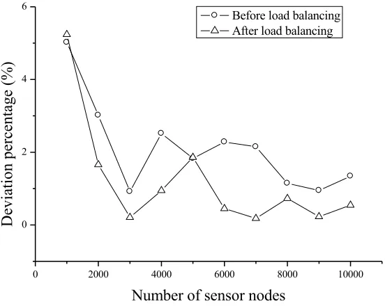
Figure 2 is the comparison of load balancing when the number of Sink nodes is 4. The horizontal coordinate shows the sensor node deployment number from 1000 to

k k

k

=

N

N

g

t k

k res SH

b

d

E

P

10000, and the vertical coordinate suggest the deviation between 4 Sink nodes and av-erage number of nodes before and after load balancing.

Fig. 1. The implementation results based on Inter-Area Load Balancing algorithm

Fig. 2. The comparison of deviation results of Sink nodes before and after load balancing

0 50 100 150 200 250

Sink node number

N

o.

each S

in

k i

s responsi

bl

e for

Before load balancing After load balancing

1 2 3 4

0 2000 4000 6000 8000 10000 0

2 4 6

D

eviation percentage (%

)

Number of sensor nodes

From the figure, it can be seen that, after load balancing, the deviation percentage between Sink node and average number of nodes is smaller than that before load bal-ancing. And with the increase of the number of sensor nodes, that is, the density of nodes in the area becomes larger, the comparison of two deviation percentage lines shows good distance. It proves that Inter-Area Load Balancing algorithm has good ex-tensibility in terms of load balancing effect between large-scale sensor networks.

Three ideal Sink nodes are deployed in the same area. It is supposed that the rectan-gle border length is 50m, the center of the circular area is three Sink nodes arranged in triangle and the distance is 5m, and they constitute an equilateral triangle topology. Ordinary sensor nodes are circular, and ideally, they are evenly partitioned into three sector regions by three Sink. Figure 3 shows the comparison of the number of nodes in the three Sink before and after using the Inter-Area Load Balancing algorithm. The total number of sensor nodes in the area is 900.

Fig. 3. The comparison of the number of nodes in the three Sink before and after using the In-ter-Area Load Balancing algorithm

It can be seen from the figure that, the number of nodes numbered 1 Sink possessed before the load balancing is more than 300 of the average value, and more than the other two Sink. After the load balancing, the number of nodes that 3 Sink possessed is approximately equal and close to 300. This shows that the Inter-Area Load Balancing algorithm can effectively reduce the number of nodes that Sink has with a heavier load and balance the number of sensor nodes that the rest of the Sink has in the same area.

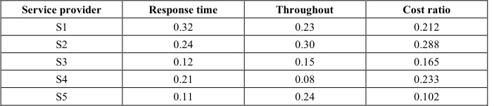
Next, the quality of service in the cloud core layer in the SVC4WSN architecture is considered. From the above theoretical analysis, it is seen that the parameters affecting service quality are response time, throughput and cost ratio, respectively. Assuming that there are 5 different services running on a virtual machine platform, they have dif-ferent quality of service parameters, as shown in Table 1:

0 50 100 150 200 250 300 350

Sink node number

N

o.

each S

in

k i

s responsi

bl

e for

Before load balancing After load balancing

Table 1. The parameters of quality of service for 5 services (obtained over the same period)

Service provider Response time Throughout Cost ratio

S1 0.32 0.23 0.212

S2 0.24 0.30 0.288

S3 0.12 0.15 0.165

S4 0.21 0.08 0.233

S5 0.11 0.24 0.102

It can be found from the table that S1 takes the longest response time in the same time period, and S2 can get the maximum throughput on the virtual machine, but S2 spend the most virtual machine resources and S5 spend the least resource. Using the formula of computing service Rank value provided in the algorithm, the service Rank value and service sequencing shown in Table 2 can be obtained.

Table 2. The order of Rank value of 5 services (a=0.4, b=0.2, c=0.4)

Service provider Service Rank Service order

S1 0.2588 4

S2 0.2712 5

S3 0.144 2

S4 0.1932 3

S5 0.1328 1

In the case of a=c=0.4 and b=0.2, the service with the lowest Rank value is S5. At this time, the service Rank is more concerned with response time and resource cost, so a and c are valued larger than b. Selecting a smaller throughput weight b can reduce the effect of the throughput rate on the service Rank value. It is also what the virtual plat-form expects for the quality of service, that is, to achieve higher service throughput when the response time and the platform resource cost ratio is small, which is the basis of the Rank values of service S5 ranked No.1. If the response time threshold and throughput threshold of the virtual machine platform are set at 20%, then the response time and throughput rates of service S1 and S2 are higher than the set threshold. If the cost ratio of the two service platforms does not exceed the cost state value of the current virtual machine (VM) platform (this is a variable, depending on the number of services running on the VM platform simultaneously), then S1 and S2 will be transferred to a new VM platform; otherwise, the operation of services S1 and S2 will be suspended.

4.2 Experimental simulation and discussion of MDF4LWSN frame

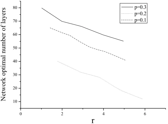
Fig. 4. The relationship between the optimal number of network layers and the unit communi-cation radius

Figure 4 shows the relationship between the network optimal layer number L and the node communication radius r_com in the circular range of the radius R=100m in the case of different node density P (number of nodes contained in per square meter). The node density P varies from 0.1 to 0.3, representing the dashed line at the top when p is 0.3, and the dashed line at the bottom when p is 0.1. It can be seen from the figure that with the decrease of node density p, the communication radius between nodes will gradually increase, and the corresponding optimal number of layers will decrease. This is because, in order to minimize the total energy consumed by the whole network, the possibility of communication between nodes is increased and the distance between the nodes is closer in the case of the number of node increasing. Therefore, the communi-cation radius r_com of the node will become smaller and the network optimal layer number L will increase, and L will be obtained when the optimal value ESUM is the

minimum. The dotted lines with high P values are above the dotted lines with low p values, which shows that when the node communication radius is constant, the nodes need more layers to make the whole network less energy-consuming.

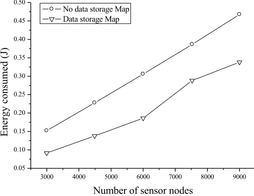
Consider the relationship between energy Reduce path and data storage Map. The design purpose of energy Reduce path design is to minimize the energy consumption between storage head (SH) nodes. In the area where radius R=100m, there are 3000 nodes in total, and the node density value is about 0.1. When the node communication radius r_com equals 2m, the optimal layer number of the network is 40 layers. The number of bits per second of each node is 100bit/s. In the case of time T=10s, Figure 5 shows the effect of the data storage Map on the energy consumed by the energy Reduce path.

0 2 4 6

10 20 30 40 50 60 70 80

N

et

w

or

k

opt

im

al

num

ber

of

la

yer

s

r

Fig. 5. The relationship between data storage Map and energy Reduce path

As can be seen from the figure that, the energy consumed by the whole network under the action of the energy Reduce path has a significant downward trend when there is a data storage Map. This is because in the data storage Map, a space time map is taken to the node, so that the sub nodes belonging to the same SH node only collect the data belonging to their own time slot. Although the burden of the SH node is increased, the energy of the whole network is saved by the existence of the backbone path. From the two curves, it is seen that, as the number of nodes increases, the energy consumption is greater. But in general, the increase of energy consumption is proportional to the increase of the number of nodes. This shows that the number of nodes on the backbone path is not significantly changed in the construction of the energy Reduce path, and the most energy consumption is the node collecting data and the SG node.

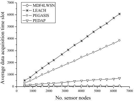
Finally, the performance of the Reduce path in the MDF4LWSN framework is dis-cussed, and it is compared with the three protocols of LEACH, PEGASIS and PEDAP. Figure 6 shows the performance of data acquisition delay under four different protocols. The time slot number of data acquisition based on the time delay Reduce path is the smallest. The reason is that in this case, the number of time slots is the logarithm of the number of nodes, and with the increase of the number of nodes, the number of time slot is maintained in a stable state. PEDAP is followed by it in terms of the delay perfor-mance, which is larger than MDF4LWSN, and they are tree topology. But PEDAP can-not guarantee that the parent node does can-not have to wait for the time slot completion of the brother node when the data is received. Therefore, the tree topology constructed with the shortest path algorithm does not have the optimal transmission delay in the PEDAP. The number of time slots collected by PEGASIS is much higher than that of the previous two algorithms, because in the link, it takes more time to transfer data from the terminal node to the middle head node in the link. The delay performance of

3000 4000 5000 6000 7000 8000 9000 0.05

0.10 0.15 0.20 0.25 0.30 0.35 0.40 0.45 0.50

Energy consum

ed (J)

Number of sensor nodes No data storage Map

Fig. 6. The performance of data acquisition delay under four different protocols

5

Conclusion

On the basis of the comprehensive analysis of WSN and cloud computing technol-ogy, some suggestions on the architecture of WSN based on cloud computing and the large-scale data processing scheme are put forward. The large-scale WSN architecture based on cloud computing and the mass data processing framework in the WSN is stud-ied.

The effect of multi-Sink mechanism on the load balancing of WSN nodes is dis-cussed through simulation experiments, and the comparison of the results before and after load balancing is carried out. In the Map part of the network structure, the rela-tionship between the optimal number of nodes and the communication radius of nodes under different node densities is verified by simulation. The experiment simulates the influence of data storage Map on network energy consumption. Finally, the energy and delay Reduce paths are discussed and compared with the three protocols of LEACH, PEGASIS and PEDAP in simulation.

6

References

[1]Arora, V. K., Sharma, V., & Sachdeva, M. (2016). A survey on leach and other's rout-ing protocols in wireless sensor network. Optik, 127(16): 6590-6600. https://doi.org/10.1016/ j.ijleo.2016.04.041

[2]Zahurul, S., Mariun, N., Grozescu, I. V., Tsuyoshi, H., Mitani, Y., & Othman, M. L., et al. (2016). Future strategic plan analysis for integrating distributed renewable genera-tion to smart grid through wireless sensor network: malaysia prospect. Renewable & Sustainable Energy Reviews, 53: 978-992. https://doi.org/10.1016/j.rser.2015.09.020

0 1000 2000 3000 4000 5000 6000 7000

0 1000 2000 3000 4000 5000 6000 7000

A

verage data acquisition tim

e slot

No. sensor nodes

[3]Olofsson, T., Ahlén, A., & Gidlund, M. (2016). Modeling of the fading statistics of wireless sensor network channels in industrial environments. IEEE Transactions on Signal Pro-cessing, 64(12): 3021-3034. https://doi.org/10.1109/TSP.2016.2539142

[4]Wei, W., Song, H., Li, W., Shen, P., & Vasilakos, A. (2017). Gradient-driven parking navi-gation using a continuous information potential field based on wireless sensor network. In-formation Sciences, 408(C): 100-114. https://doi.org/10.1016/j.ins.2017.04.042

[5]Khasawneh, A., Latiff, M. S. B. A., Kaiwartya, O., & Chizari, H. (2017). A reliable en-ergy-efficient pressure-based routing protocol for underwater wireless sensor net-work. Wireless Networks, 1-15.

[6]Kumar, R., & Kumar, D. (2016). Multi-objective fractional artificial bee colony algo-rithm to energy aware routing protocol in wireless sensor network. Wireless Net-works, 22(5): 1461-1474. https://doi.org/10.1007/s11276-015-1039-4

[7]Mai, A., Liang, Y., & Li, T. (2016). Mobile coordinated wireless sensor network: an energy efficient scheme for real-time transmissions. IEEE Journal on Selected Areas in Communi-cations, 34(5): 1663-1675. https://doi.org/10.1109/JSAC.2016.2545383

[8]Gasparri, A., Krishnamachari, B., & Wang, S. (2016). Throughput-optimal robotic message ferrying for wireless sensor network using coarse-grained backpressure con-trol. IEEE Transactions on Mobile Computing, 16(2): 1-1.

[9]Ghari, P. M., Shahbazian, R., & Ghorashi, S. A. (2016). Wireless sensor network local-ization in harsh environments using sdp relaxation. IEEE Communications Letters, 20(1): 137-140. https://doi.org/10.1109/LCOMM.2015.2498179

[10]Zhang, Z., Glaser, S. D., Bales, R. C., Conklin, M., Rice, R., & Marks, D. G. (2017). Tech-nical report: the design and evaluation of a basin-scale wireless sensor network for mountain hydrology. Water Resources Research, 53(5): 4487-4498. https://doi.org/10.1002/201 6WR019619

7

Author

Qiong Ren works as associate professor at School of Mathematics and Computer Science, Jianghan University, Wuhan, 430056, China.