The Thirty-Third AAAI Conference on Artificial Intelligence (AAAI-19)
Gradient Harmonized Single-Stage Detector
Buyu Li,
∗Yu Liu,
∗Xiaogang Wang
{byli, yuliu, xgwang}@ee.cuhk.edu.hk
Multimedia Laboratory, The Chinese University of Hong Kong, Hong Kong
Abstract
Despite the great success of two-stage detectors, single-stage detector is still a more elegant and efficient way, yet suffers from the two well-known disharmonies during training, i.e. the huge difference in quantity between positive and nega-tive examples as well as between easy and hard examples. In this work, we first point out that the essential effect of the two disharmonies can be summarized in term of the gradient. Further, we propose a novel gradient harmonizing mechanism (GHM) to be a hedging for the disharmonies. The philoso-phy behind GHM can be easily embedded into both classi-fication loss function like cross-entropy (CE) and regression loss function like smooth-L1 (SL1) loss. To this end, two
novel loss functions called GHM-C and GHM-R are designed to balancing the gradient flow for anchor classification and bounding box refinement, respectively. Ablation study on MS COCO demonstrates that without laborious hyper-parameter tuning, both GHM-C and GHM-R can bring substantial im-provement for single-stage detector. Without any whistles and bells, the proposed model achieves 41.6 mAP on COCO test-devset which surpass the state-of-the-art method, Focal Loss (FL) +SL1, by 0.8. The code1is released to facilitate future
research.
1
Introduction
One-stage approach is the most efficient and elegant frame-work for object detection. But for a long time, the perfor-mance of one-stage detectors has a large gap from that of two-stage detectors. The most challenging problem for the training of one-stage detector is the serious imbalance be-tween easy and hard examples as well as that bebe-tween pos-itive and negative examples. The huge number of easy and background examples tend to overwhelm the training. But these problems are not existed for two-stage detectors, ow-ing to the proposal-driven mechanism. To handle the former imbalance problem, example mining based methods such as OHEM (Shrivastava, Gupta, and Girshick 2016) are in common use, but they directly abandon most examples and the training is inefficient. For the latter imbalance, the re-cent work, Focal Loss (Lin et al. 2017b), has tried to ad-dress it by rectifying the cross-entropy loss function to a
∗
They contributed equally to this work
Copyright c2019, Association for the Advancement of Artificial Intelligence (www.aaai.org). All rights reserved.
1
https://github.com/libuyu/GHM Detection
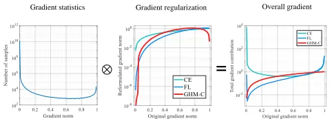
Gradient statistics Gradient regularization Overall gradient
Figure 1: An illustration of gradient harmonizing mecha-nism. The figure in the left displays the distribution of rela-tive gradient norm in a converged model in log scale respec-tively. The middle figure displays the new gradient norms after the rectification of Focal Loss (FL) and GHM-C loss, compared with the original cross-entropy (CE) loss. The right figure shows the total gradient contribution of exam-ples w.r.t gradient norm.
elaborately designed form. However, Focal Loss adopts two hyper-parameters which should be tuned with a lot of ef-forts. And it is a static loss which is not adaptive for the changing of data distribution, which varies along with the training process.
In this work, we first point out that the class imbalance can be summarized to the imbalance in difficulty and the imbalance in difficulty can be summarized to the imbalance in gradient norm distribution. If a positive example is well-classified, it is an easy example and the model benefit little from it, i.e. a little magnitude of gradient will be produced by this sample. And a misclassified example should attract attention of the model no matter which class it belongs to. So if viewed globally, the large amount of negative examples tends to be easy to classify and the hard examples are usu-ally positive. So the two kind of imbalance can be roughly summed up as attribute imbalance.
Moreover, we claim that the imbalance of examples with different attributes (hard/easy and pos/neg) can be implied by the distribution of gradient norm. The density of
exam-ples w.r.t. gradient norm, which we call asgradient density
contribution on the global gradient than a hard example, the total contribution of the huge amount of easy examples can overwhelm the contribution of the minority of hard exam-ples and the training process will be inefficient. Besides, we also discover that the density of examples with very large gradient norm (very hard examples) is slightly larger than the density of the medium examples. And we consider these very hard examples mostly as outliers since they exist stably even when the model is converged. The outliers may affect the stability of model since their gradients may have a large discrepancy from the other common examples.
Inspired by the analysis of gradient norm distribution, we propose a gradient harmonizing mechanism (GHM) to train the one-stage object detection model in an efficient, which focuses on the harmony of gradient contribution of different examples. The GHM first performs statistics on the number of examples with similar attributes w.r.t their gradient den-sity and then attach a harmonizing parameter to the gradi-ent of each example according to the density. The effect of GHM compared with CE and FL is illustrated in the right of Fig.1. Training with GHM, the huge amount of cumulated gradient produced by easy examples can be largely down-weighted and the outliers can be relatively down-down-weighted as well. In the end, the contribution of each kind of exam-ples will be balanced and the training can be more efficient and stable.
In practice, the modification of gradient can be equiva-lently implemented by reformulating the loss function, we embed the GHM into the classification loss, which is de-noted as GHM-C loss. This loss function is elegantly for-mulated without many hyper-parameters to tune. Since the gradient density is a statistical variable depending on the ex-amples distribution in a mini-batch, GHM-C is a dynamic loss that can adapt to the change of data distribution in each batch as well as to the updating of model. To showcase the generality of GHM, we also adopt it in the box regression branch as the form of GHM-R loss.
Experiments on the bounding box detection track of the challenging COCO benchmark show that the GHM-C loss has a large gain compared to the traditional cross-entropy loss and slightly surpasses the state-of-the-art Focal Loss. And the GHM-R loss also has better performance than the
commonly used smoothL1loss. The combination of
GHM-C and GHM-R attains a new state-of-the-art performance on COCOtes-devset.
Our main contributions are as follows:
1. We reveal the essential principle behind the significant example imbalance in one-stage detector in term of gra-dient norm distribution, and propose a novel gragra-dient harmonizing mechanism (GHM) to handle it.
2. We embed the GHM into the loss for classification and regression as GHM-C and GHM-R respectively, which rectify the gradient contribution of examples with differ-ent attributes and is robust to hyper-parameters.
3. Collaborating with GHM, we can easily train a single stage detector without any data sampling strategy and achieve the state-of-the-art result on COCO benchmark.
2
Related Work
Object Detection: Object detection is one of the most ba-sic and important task in the field of computer vision. Deep convolutional neural network (CNN) based methods, e.g. (Ren et al. 2015; Liu et al. 2016; Redmon and Farhadi 2017; He et al. 2017), have become more and more developed and achieved great success in recent years, owing to the signif-icant progress of network architecture such as (Simonyan and Zisserman 2014; Szegedy et al. 2016; He et al. 2016; Huang et al. 2017). Advanced object detection frameworks can be divided into two categories: one-stage detector and two-stage detector.
Most state of the art methods use two-stage detectors, e.g. (Girshick 2015; Ren et al. 2015; Li et al. 2017; He et al. 2017; Lin et al. 2017a; Zeng et al. 2018). They are mainly based on the Region CNN (R-CNN) architecture. These ap-proaches first obtain a manageable number of region pro-posals called region of interest (RoI) from the nearly infinite candidate regions and then use the network to evaluate each RoI.
One-stage detectors have the advantage of simple struc-tures and high speed. SSD (Liu et al. 2016; Fu et al. 2017), YOLO (Redmon et al. 2016; Redmon and Farhadi 2017; 2018) for generic object detection and RSA (Song et al. ; Liu et al. 2017) for face detection have achieved good speed/accuracy trade-off. However, they can hardly surpass the accuracy of two-stage detectors. RetinaNet (Lin et al. 2017b) is the state of the art one-stage object detector that achieve comparable performance to two-stage detectors. It adopts an architecture modified from RPN (Ren et al. 2015) and focuses on addressing the class imbalance during train-ing.
Object Functions for Object Detector: Most detection models use cross entropy based loss function for classifi-cation (Girshick 2015; Ren et al. 2015; Liu et al. 2016; Dai et al. 2016; Lin et al. 2017a; He et al. 2017). While one-stage detectors face a problem of extreme class imbalance that two-stage detectors do not have. Earlier methods try to use hard example mining methods, e.g. (Shrivastava, Gupta, and Girshick 2016; Felzenszwalb, Girshick, and McAllester 2010), but they discard most examples and cannot handle the problem well. Recently the work (Lin et al. 2017b) reformu-late the cross-entropy loss so that easy negatives are down-weighted and the hard examples are unaffected or even up-weighted.
For stable training of box regression, Fast R-CNN
(Gir-shick 2015) introduces the smoothL1loss. This loss reduces
the impact of outliers so that the training of model can be more stable. Almost all the following works take the smooth
L1 loss as a default for box regression (Ren et al. 2015;
Liu et al. 2016; Dai et al. 2016; Lin et al. 2017a; He et al. 2017).
Our GHM based loss harmonizes the contribution of ex-amples on the basis of the distribution of their gradient, so that it can handle both the class imbalance and the outliers problem well. It can also adapt the weights to the changing of data distribution in each mini-batch.
3
Gradient Harmonizing Mechanism
Problem Description
Similar to (Lin et al. 2017b), our efforts here are focused on classification in one-stage object detection where the classes (foreground/background) of examples are quite imbalanced.
For a candidate box, letp ∈ [0,1]be the probability
pre-dicted by the model and p∗ ∈ {0,1} be its ground-truth
label for a certain class. Consider the binary cross entropy loss:
LCE(p, p∗) =
−log(p) ifp∗= 1
−log(1−p) ifp∗= 0 (1)
Let x be the direct output of the model such that p =
sigmoid(x), we have the gradient with regard to x:
∂LCE
∂x =
p−1 ifp∗= 1
p ifp∗= 0
=p−p∗
(2)
We definegas follows:
g=|p−p∗|=
1−p ifp∗= 1
p ifp∗= 0 (3)
gequals to the norm of gradient w.r.tx. The value ofg
repre-sents attribute (e.g. easy or hard) of an example and implies the example’s impact on the global gradient. Although the strict definition of gradient is on the whole parameter space,
which meansgis a relative norm of an example’s gradient,
we callgas gradient norm in this paper for convenience.
Fig.2 shows the distribution ofg from a converged
one-stage detection model. Since the easy negatives have a dom-inant number, we use log axis to display the fraction of ex-amples to demonstrate the details of the variance of exam-ples with different attributes. It can be seen that the number of very easy examples is extremely large, which have a great impact on the global gradient. Moreover, we can see that a converged model still can’t handle some very hard examples whose number is even larger than the examples with medium difficulty. These very hard examples can be regarded as out-liers since their gradient directions tends to vary largely from the gradient directions of the large amount of other exam-ples. That is, if the converged model is forced to learn to classify these outliers better, the classification of the large number of other examples tends to be less accurate.
Gradient Density
To handle the problem of the disharmony of gradient norm distribution, we introduce a harmonizing approach with re-gard to gradient density. Gradient density function of train-ing examples is formulated as Equation.4:
GD(g) = 1
l(g)
N X
k=1
δ(gk, g) (4)
0 0.2 0.4 0.6 0.8 1
gradient norm 10-6
10-4 10-2 100
fraction of examples
Figure 2: The distribution of the gradient normgfrom a
con-verged one-stage detection model. Note that the y-axis uses log scale since the number of examples with different gradi-ent norm can differ by orders of magnitude.
wheregkis the gradient norm of the k-th example. And
δ(x, y) =
(
1 ify−
2 <=x < y+
2
0 otherwise
(5)
l(g) = min(g+
2,1)−max(g−
2,0) (6)
The gradient density ofgdenotes the number of examples
lying in the region centered atgwith a length ofand
nor-malized by the valid length of the region.
Now we define the gradient density harmonizing parame-ter as:
βi= N
GD(gi) (7)
whereN is the total number of examples. To better
com-prehend the gradient density harmonizing parameter, we can
rewrite it asβi=GD(g1
i)/N. The denominatorGD(gi)/Nis
a normalizer indicating the fraction of examples with neigh-borhood gradients to the i-th example. If the examples are
uniformly distributed with regard to gradient,GD(gi) =N
for any gi and each example will have the same βi = 1,
which means nothing is changed. Otherwise, the examples with large density will be relatively down-weighted by the normalizer.
GHM-C Loss
We embed the GHM into classification loss by regardingβi
as the loss weight of the i-th example and the gradient den-sity harmonized form of loss function is:
LGHM−C =
1
N N X
i=1
βiLCE(pi, p∗i)
=
N X
i=1
LCE(pi, p∗i) GD(gi)
(8)
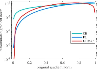
Fig.3 illustrates the reformulated gradient norm of dif-ferent losses. Here we take the original gradient norm of
since the density is calculated according to g. We can see that the curves of Focal Loss and GHM-C loss have similar trend, which implies that Focal Loss with the best hyper-parameters is similar with uniform gradient harmonizing. Furthermore, GHM-C has one more merit that Focal loss ig-nores: down-weighting the gradient contribution of outliers.
0 0.2 0.4 0.6 0.8 1
original gradient norm 10-8
10-6 10-4 10-2 100
reformulated gradient norm
CE FL GHM-C
Figure 3: Reformulated gradient norm of different loss
func-tions w.r.t the original gradient normg. The y-axis uses log
scale to better display the details of FL and GHM-C.
With our GHM-C loss, the huge number of very easy examples are largely down-weighted and the outliers are slightly down-weighted as well, which simultaneously ad-dresses the attribute imbalance problem and the outliers problem. From the right figure in Fig.1 we can better see that GHM-C harmonizes the total gradient contribution of different group of examples. Since the gradient density is calculated every iteration, the weights of examples are not
fixed w.r.t.g (or x) like focal loss but adaptive to current
state of model and mini-batch of data. The dynamic prop-erty of GHM-C loss makes the training more efficient and robust.
Unit Region Approximation
Complexity Analysis: The naive algorithm to calculate the gradient density values of all examples has a time
com-plexity ofO(N2), which can be easily attained from
Equa-tions 4 and 8. Even parallel computed, each computing unit
still bears a computation ofN. And as far as we know, the
best algorithm first sort the examples by gradient norm with
a complexity ofO(NlogN)and then use a queue to scan
the examples and get their density withO(N). This sorting
based method can not gain much from parallel computing.
Since N of an image in one-stage detector can be 105 or
even106, to directly calculate the gradient density is quite
time consuming. So we introduce an alternative approach to approximately attain the gradient density of examples.
Unit Region: We divide the range space ofginto
individ-ual unit regions with a length of , and there areM = 1
unit regions. Letrj be the unit region with index j so that
rj = [(j−1), j). LetRj denote the number of examples
lying inrj. We defineind(g) =ts.t.(t−1) <=g < t,
which is the index function to the unit region thatglies in.
Then we define the approximate gradient density function as:
ˆ
GD(g) =Rind(g)
=Rind(g)M (9)
Then we have the approximate gradient density harmonizing parameter:
ˆ
βi= N
ˆ
GD(gi) (10)
Consider the special case where= 1: there are just one unit
region and all examples lie in it, so obviously everyβi = 1
and each example keep their original gradient contribution. Finally we have the reformulated loss function:
ˆ
LGHM−C =
1
N N X
i=1 ˆ
βiLCE(pi, p∗i)
=
N X
i=1
LCE(pi, p∗i)
ˆ
GD(gi)
(11)
From Equation. 9 we can see that the examples lying in the same unit region share the same gradient density. So we can use the algorithm of histogram statistics and the compu-tation of all the gradient density values has a time
complex-ity of O(M N). And parallel computing can be applied so
that each computing unit has a computation ofM. In
prac-tice, we can attain good performance with quite small
num-ber of unit regions. That isM is fairly small and the
calcu-lation of loss is efficient.
EMA: Mini-batch statistics based methods usually face a
problem: when many extreme data are just sampled in one mini-batch, the statistical result will be a serious noise and the training will be unstable. Exponential moving average (EMA) is a common used method to address this problem, e.g., SGD with momentum (Sutskever et al. 2013) and Batch Normalization (Ioffe and Szegedy 2015). Since in the ap-proximation algorithm the gradient densities come from the numbers of examples in the unit regions, we can apply EMA on each unit region to obtain more stable gradient densities
for examples. LetR(jt)be the number of examples in the
j-th unit region in j-the t-j-th iteration and Sj(t) be the moving
averaged number. We have:
S(jt)=αSj(t−1)+ (1−α)R(jt) (12)
whereαis the momentum parameter. We use the averaged
numberSjto calculate the gradient density instead ofRj:
ˆ
GD(g) = Sind(g)
=Sind(g)M (13)
With EMA, the gradient density will be more smooth and insensitive to extreme data.
GHM-R Loss
Consider the parameterized offsets, t = (tx, ty, tw, th),
predicted by box regression branch and the target offsets,
t∗ = (t∗x, ty∗, t∗w, t∗h), computed from ground-truth. The
re-gression loss usually adopts the smoothL1loss function:
Lreg = X
i∈{x,y,w,h}
where
SL1(d) =
d2
2δ if|d|<=δ
|d| −δ
2 otherwise
(15)
whereδ is the division point between the quadric part and
the linear part, and usually set to1/9in practice.
Sinced=ti−t∗i, the gradient of smoothL1loss w.r.tti
can be expressed as:
∂SL1
∂ti =
∂SL1
∂d =
d
δ if|d|<=δ
sgn(d) otherwise
(16)
wheresgnis the sign function.
Note that all the examples with|d|larger than the division
point have the same gradient norm|∂SL1
∂ti |= 1, which makes
the distinguishing of examples with different attributes im-possible if depending on the gradient norm. An alternative
choice is directly using|d|as the measurement of different
attributes, but the new problem is|d|can reach to infinite in
theory and the unit region approximation can not be imple-mented.
To conveniently apply GHM on regression loss, we first
modify the traditionalSL1loss into a more elegant form:
ASL1(d) =
p
d2+µ2−µ (17)
This loss shares similar property with SL1 loss: when d
is small it approximates a quadric function (L2 loss) and
when d is large is approximate a linear function (L1 loss).
We denote the modified loss function as Authentic Smooth
L1(ASL1) loss for its good property of authentic
smooth-ness, which means all the degrees of derivatives are existed and continuous. In contrast, the second derivative of smooth
L1loss does not exist at the pointd =δ. Furthermore, the
ASL1loss has an elegant form of gradient w.r.td:
∂ASL1
∂d =
d p
d2+µ2 (18)
The range of the gradient is just [0,1), so the calculation
of density in unit regions forASL1loss in regression is as
convenient as CE loss in classification. In practice, we set
µ= 0.02forASL1loss to keep the same performance with
SL1loss.
We definegr=|√ d
d2+µ2|as the gradient norm ofASL1
loss and the gradient distribution of a converged model is il-lustrated in Fig.4 We can see that there are large number of outliers. Note that the regression is only performed on the positive examples so it is reasonable for the different dis-tribution trend between classification and regression. Above all, we can apply GHM on regression loss:
LGHM−R=
1
N N X
i=1
βiASL1(di)
=
N X
i=1
ASL1(di)
GD(gri)
(19)
0 0.2 0.4 0.6 0.8 1
gradient norm 0.02
0.04 0.06 0.08 0.1
fraction of examples
Figure 4: The distribution of the gradient normgrforASL1
loss.
0 0.05 0.1 0.15 0.2
error to ground truth 0
0.2 0.4 0.6 0.8 1
reformulated gradient norm
SL1 ASL1 GHM-R
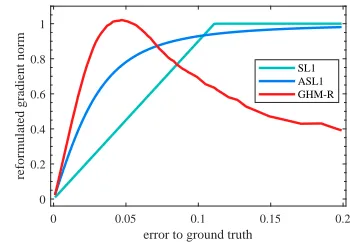
Figure 5: Comparison of the reformulated gradient
contribu-tions of different regression losses w.r.t the value of|d|, i.e.
the error to ground-truth.
The reformulated gradient contribution of SL1 loss,
ASL1loss and GHM-R loss in Fig.5. The x-axis adopts|d|
for convenient comparison.
We emphasize that in box regression not all the “easy ex-amples” are unimportant. An easy example in classification is usually a background region with a very low predicted probability and will be definitely excluded from the final candidates. Thus the improvement of this kind of examples makes nearly no contribution to the precision. But in box re-gression, an easy example still has deviation from the ground truth location. Better prediction of any example will directly improve the quality of the final candidates. Moreover, ad-vanced datasets care more about the localization accuracy. For example, COCO (Lin et al. 2014) takes the average AP from the IoU threshold 0.5 to 0.95 as the metric to evaluate an algorithm. In this metric, the some of the so called easy examples (those having small errors) are also important be-cause reducing the errors of them can directly improve the AP at high threshold (e.g. AP@IoU=0.75).
Our GHM-R loss can harmonize the contribution of easy and hard examples for box regression by up-weighting the important part of easy examples and down-weighting the outliers. Experiments show that it can attain better
4
Experiments
We evaluate our approach on the challenging COCO bench-mark (Lin et al. 2014). For training, we follow the common used practice (He et al. 2017; Lin et al. 2017b) to divide the 40k validation set into a 35k subset and a 5k subset. The union of the 35k validation subset and the whole 80k training
set are used for training together and denoted astrainval35k
set. The 5k validation subset is denoted asminivalset and
our ablation study is performed on it. While our main results
are reported on thetest-devset.
Implementation Details
Network Setting: We use RetinaNet (Lin et al. 2017b) as network architecture and all the experiments adopt ResNet (He et al. 2016) as backbone with Feature Pyramid Network (FPN) (Lin et al. 2017a) structure. Anchors use 3 scales and 3 aspect ratios for convenient comparison with focal loss. The input image scale is set as 800 pixel for all experiments. For all ablation studies, ResNet-50 is used. While the
fi-nal model evaluated ontest-devadopts ResNeXt-101 (Hu,
Shen, and Sun 2017). In contrast to focal loss, our approach doesn’t need a specialized bias initialization.
Optimization: All the models are optimized by the com-mon used SGD algorithm. We train the models on 8 GPUs with 2 images on each GPU so that the effective mini-batch size is 16. All models are trained for 14 epochs with an ini-tial learning rate of 0.01, which is decreased by a factor 0.1 at the 9th epoch and again at the 12th epoch. We also use a weight decay parameter of 0.0001 and a momentum param-eter of 0.9. The only data augmentation operation is hori-zontal image flipping. For the EMA used in gradient density
calculation, we useα= 0.75for all experiments since the
results are insensitive to the exact value ofα.
GHM-C Loss
To focus on the effect of GHM-C loss function, experiments
in this section all adopt smoothL1 loss function withδ =
1/9for the box regression branch.
Baseline: We have trained a model with the standard cross entropy loss as the baseline. The standard initialization will lead to quick divergence, so we follow focal loss (Lin et al. 2017b) to initialize the bias term of the last layer to b =−log((1−π)/π)withπ= 0.01to avoid divergence. However with the specialized initialization the loss of classi-fication is very small, so we up-weight the classiclassi-fication loss by 20 to make the begging loss value reasonable (the beg-ging classification loss value is around 1 now). But when the model converge, the classification loss is still very small and we finally obtain a model with an Average Precision (AP) of 28.6.
Number of Unit Region Table.1 shows the results of
varying M which is the number of unit regions. EMA is
not applied here. WhenM is too small, the density can not
have a good variation over different gradient norm and the
performance is not so good. So we can gain more whenM
increases whenM is not large. HoweverM is not
necessar-ily very large, whenM = 30, the GHM-C loss yields a large
enough improvement over baseline.
M AP AP.5 AP.75 APS APM APL
5 33.4 51.7 35.6 18.6 36.8 45.7
10 34.6 53.9 36.5 19.5 37.1 46.1
20 35.2 54.4 36.9 19.4 38.4 46.3
30 35.8 55.5 38.1 19.6 39.6 46.7
40 35.4 54.8 36.3 19.5 38.5 46.3
Table 1: Results of varying number of unit regions for GHM-C loss.
Speed: Since our approach is a loss function, it doesn’t
change the time for inference. For training, a smallM of 30
is enough to attain good performance, so time consumed by gradient density calculation is not long. Table.2 shows the average time for each iteration during training as well as av-erage precision. Here “GHM-C Standard” is implemented using the original definition of gradient density and “GHM-C RU” represents the implementation of region unit approxi-mation algorithm. The experiments are performed on 1080Ti GPUs. We can see that our region unit approximation algo-rithm speed up the training by magnitudes with negligible harm to performance. While compared with CE, the slow down of GHM-C loss is also acceptable. Since our loss is not fully GPU implemented now, there is still room for im-provement.
method AP average time per iteration (s)
standard CE 28.6 0.566
GHM-C Standard 35.9 13.675
GHM-C RU 35.8 0.824
Table 2: The comparison of training speed as well as AP.
Comparison with Other Methods: Table.4 shows the re-sults using our loss compared with other loss functions or
sampling strategy. Since the reported results onminivalof
models using focal loss is trained with the input image scale of 600 pixels, for fair comparison we have re-trained a focal loss using a scale of 800 pixels and keep the best parameters of focal loss. We can see our loss has slightly better perfor-mance than focal loss.
GHM-R Loss
Comparison with Other Losses: The experiments here adopt the best configuration of GHM-C loss for the classi-fication branch. So the first baseline is the model (trained
usingSL1loss) with an AP of 35.8 showed in GHM-C loss
experiments. We adoptsµ= 0.02forASL1loss to get
com-parable results withSL1loss and obtain a fair baseline for
GHM-R loss. Table.5 shows the results of the baselineSL1
andASL1loss as well as GHM-R loss. We can see a gain of
method network AP AP50 AP75 APS APM APL
Faster RCNN (Ren et al. 2015) FPN-ResNet-101 36.2 59.1 39.0 18.2 39.0 48.2
Mask RCNN (He et al. 2017) FPN-ResNet-101 38.2 60.3 41.7 20.1 41.1 50.2
Mask RCNN (He et al. 2017) FPN-ResNeXt-101 39.8 62.3 43.4 22.1 43.2 51.2
YOLOv3 (Redmon and Farhadi 2018) DarkNet-53 33.0 57.9 34.4 18.3 35.4 41.9
DSSD513 (Fu et al. 2017) DSSD-ResNet-101 33.2 53.3 35.2 13.0 35.4 51.1
Focal Loss (Lin et al. 2017b) RetinaNet-FPN-ResNet-101 39.1 59.1 42.3 21.8 42.7 50.2
Focal Loss (Lin et al. 2017b) RetinaNet-FPN-ResNeXt-101 40.8 61.1 44.1 24.1 44.2 51.2
GHM-C + GHM-R (ours) RetinaNet-FPN-ResNet-101 39.9 60.8 42.5 20.3 43.6 54.1
GHM-C + GHM-R (ours) RetinaNet-FPN-ResNeXt-101 41.6 62.8 44.2 22.3 45.1 55.3
Table 3: Comparison with state-of-the-art methods (single model) on COCOtest-devset.
method AP AP.5 AP.75 APS APM APL
CE 28.6 43.3 30.7 11.4 30.7 40.7
OHEM 31.1 47.2 33.2 - -
-FL 35.6 55.6 38.2 19.1 39.2 46.3
GHM-C 35.8 55.5 38.1 19.6 39.6 46.7
Table 4: Comparison of other loss functions. Note that the ’OHEM’ is trained with ResNet-101 while others are trained with ResNet-50.
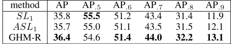
of AP at different IoU thresholds. GHM-R loss slightly low-ers the AP@IoU=0.5 but gains when the threshold is higher, which demonstrates our proposition that the so called easy examples in regression is important for accurate localization.
method AP AP.5 AP.75 APS APM APL
SL1 35.8 55.5 38.1 19.6 39.6 46.7
ASL1 35.7 55.0 38.1 19.7 39.7 45.9
GHM-R 36.4 54.6 38.7 20.5 40.6 47.8
Table 5: Comparison of different loss functions for regres-sion.
method AP AP.5 AP.6 AP.7 AP.8 AP.9
SL1 35.8 55.5 51.2 43.4 31.4 11.9
ASL1 35.7 55.0 51.1 43.5 31.5 12.1
GHM-R 36.4 54.6 51.4 44.0 32.2 13.1
Table 6: Comparison of AP at different IoU thresholds.
Two-Stage Detector: GHM-R loss for regression is not limited to one-stage detectors. So we have done experi-ments to verify the effect on two-stage detectors. Our base-line method is faster-RCNN with Res50-FPN model using
SL1loss for box regression. Table.7 shows that GHM-R loss
works for two-stage detector as well as one-stage detector.
Main Results
We use the 32x8d FPN-ResNext101 backbone and Reti-naNet model with C loss for classification and GHM-R loss for box regression. The experiments are performed on
method AP AP.5 AP.75 APS APM APL
SL1 36.4 58.7 38.8 21.1 39.6 47.0
GHM-R 37.4 58.9 39.9 21.8 40.8 48.8
Table 7: Comparison of regression loss functions on two-stage detector.
test-dev set. Table.3 shows our main result compared with state-of-the-art methods. Our approach achieves excellent performance and outperforms focal loss in most metrics.
5
Conclusion and Discussion
In this work, we focus on the two imbalance problems in single-stage detectors and summarize these two problems to the disharmony in gradient density with regard to the diffi-culty of samples. Two loss functions, C and GHM-R are proposed to conquer the disharmony in classifica-tion and bounding box regression respectively. Experiments show that the collaborate with GHM, the performance of single-stage detector can easily surpass modern state-of-the-art two-stage detectors like FPN and Mask-RCNN with the same network backbone.
Despite of the improvement of select uniform distribution to be the target, we still hold the opinion that the optimal distribution of gradient is hard to define and requires further research.
6
Acknowledgments
We sincerely appreciate the technical and GPU support from Mr. Changbao Wang, Quanquan Li and Junjie Yan at Sense-time Research. And we also acknowledge the early discus-sion with Prof. Wanli Ouyang from University of Sydney.
References
Chen, Z.; Badrinarayanan, V.; Lee, C.-Y.; and Rabinovich, A. 2017. Gradnorm: Gradient normalization for adaptive
loss balancing in deep multitask networks. arXiv preprint
arXiv:1711.02257.
Dai, J.; Li, Y.; He, K.; and Sun, J. 2016. R-fcn: Object
detec-tion via region-based fully convoludetec-tional networks. In
Felzenszwalb, P. F.; Girshick, R. B.; and McAllester, D. 2010. Cascade object detection with deformable part
mod-els. In Computer vision and pattern recognition (CVPR),
2010 IEEE conference on, 2241–2248. IEEE.
Fu, C.-Y.; Liu, W.; Ranga, A.; Tyagi, A.; and Berg, A. C.
2017. Dssd: Deconvolutional single shot detector. arXiv
preprint arXiv:1701.06659.
Girshick, R. 2015. Fast r-cnn. InProceedings of the IEEE
international conference on computer vision, 1440–1448. He, K.; Zhang, X.; Ren, S.; and Sun, J. 2016. Deep
resid-ual learning for image recognition. InProceedings of the
IEEE conference on computer vision and pattern
recogni-tion, 770–778.
He, K.; Gkioxari, G.; Doll´ar, P.; and Girshick, R. 2017.
Mask r-cnn. InComputer Vision (ICCV), 2017 IEEE
In-ternational Conference on, 2980–2988. IEEE.
Hu, J.; Shen, L.; and Sun, G. 2017. Squeeze-and-excitation
networks. arXiv preprint arXiv:1709.015077.
Huang, G.; Liu, Z.; Van Der Maaten, L.; and Weinberger, K. Q. 2017. Densely connected convolutional networks. In
CVPR, volume 1, 3.
Imani, E., and White, M. 2018. Improving regression
performance with distributional losses. arXiv preprint
arXiv:1806.04613.
Ioffe, S., and Szegedy, C. 2015. Batch normalization: Accel-erating deep network training by reducing internal covariate
shift. arXiv preprint arXiv:1502.03167.
Li, H.; Liu, Y.; Ouyang, W.; and Wang, X. 2017. Zoom out-and-in network with map attention decision for region
pro-posal and object detection. International Journal of
Com-puter Vision1–14.
Lin, T.-Y.; Maire, M.; Belongie, S.; Hays, J.; Perona, P.; Ra-manan, D.; Doll´ar, P.; and Zitnick, C. L. 2014. Microsoft
coco: Common objects in context. InEuropean conference
on computer vision, 740–755. Springer.
Lin, T.-Y.; Doll´ar, P.; Girshick, R. B.; He, K.; Hariharan, B.; and Belongie, S. J. 2017a. Feature pyramid networks for
object detection. InCVPR, volume 1, 4.
Lin, T.-Y.; Goyal, P.; Girshick, R.; He, K.; and Dollar, P.
2017b. Focal loss for dense object detection. In 2017
IEEE International Conference on Computer Vision (ICCV), 2999–3007. IEEE.
Liu, W.; Anguelov, D.; Erhan, D.; Szegedy, C.; Reed, S.; Fu, C.-Y.; and Berg, A. C. 2016. Ssd: Single shot multibox
detector. InEuropean conference on computer vision, 21–
37. Springer.
Liu, Y.; Li, H.; Yan, J.; Wei, F.; Wang, X.; and Tang, X. 2017. Recurrent scale approximation for object detection in
cnn. InIEEE international conference on computer vision,
volume 5.
Redmon, J., and Farhadi, A. 2017. Yolo9000: Better, faster,
stronger. In2017 IEEE Conference on Computer Vision and
Pattern Recognition (CVPR), 6517–6525. IEEE.
Redmon, J., and Farhadi, A. 2018. Yolov3: An incremental
improvement.arXiv preprint arXiv:1804.02767.
Redmon, J.; Divvala, S.; Girshick, R.; and Farhadi, A. 2016. You only look once: Unified, real-time object detection. In Proceedings of the IEEE conference on computer vision and pattern recognition, 779–788.
Ren, S.; He, K.; Girshick, R.; and Sun, J. 2015. Faster r-cnn: Towards real-time object detection with region proposal
net-works. InAdvances in neural information processing
sys-tems, 91–99.
Shrivastava, A.; Gupta, A.; and Girshick, R. 2016. Train-ing region-based object detectors with online hard example
mining. InProceedings of the IEEE Conference on
Com-puter Vision and Pattern Recognition, 761–769.
Simonyan, K., and Zisserman, A. 2014. Very deep
convo-lutional networks for large-scale image recognition. CoRR
abs/1409.1556.
Song, G.; Liu, Y.; Jiang, M.; Wang, Y.; Yan, J.; and Leng, B. Beyond trade-off: Accelerate fcn-based face detector with
higher accuracy. In 2018 IEEE Conference on Computer
Vision and Pattern Recognition (CVPR).
Sutskever, I.; Martens, J.; Dahl, G.; and Hinton, G. 2013. On the importance of initialization and momentum in deep
learning. InInternational conference on machine learning,
1139–1147.
Szegedy, C.; Vanhoucke, V.; Ioffe, S.; Shlens, J.; and Wojna, Z. 2016. Rethinking the inception architecture for computer
vision. InProceedings of the IEEE conference on computer
vision and pattern recognition, 2818–2826.
Zeng, X.; Ouyang, W.; Yan, J.; Li, H.; Xiao, T.; Wang, K.; Liu, Y.; Zhou, Y.; Yang, B.; Wang, Z.; et al. 2018. Crafting
gbd-net for object detection. IEEE transactions on pattern