Near-Neighbor Methods in Random Preference Completion

The Thirty-Third AAAI Conference on Artificial Intelligence (AAAI-19)

Near-Neighbor Methods in Random Preference Completion

Ao Liu

Department of Computer Science Rensselaer Polytechnic Institute

Troy, NY 12180, USA [email protected]

Qiong Wu, Zhenming Liu

Lirong Xia

Department of Computer Science Rensselaer Polytechnic Institute

Troy, NY 12180, USA [email protected]

Abstract

This paper studies a stylized, yet natural, learning-to-rank problem and points out the critical incorrectness of a widely used nearest neighbor algorithm. We consider a model withn agents (users){xi}i∈[n] and malternatives (items)

{yl}l∈[m], each of which is associated with a latent feature

vector. Agents rank items nondeterministically according to the Plackett-Luce model, where the higher the utility of an item to the agent, the more likely this item will be ranked high by the agent. Our goal is to identify near neighbors of an arbitrary agent in the latent space for prediction.

We first show that the Kendall-tau distance based kNN pro-duces incorrect results in our model. Next, we propose a new anchor-based algorithm to find neighbors of an agent. A salient feature of our algorithm is that it leverages the rank-ings of many other agents (the so-called “anchors”) to deter-mine the closeness/similarities of two agents. We provide a rigorous analysis for one-dimensional latent space, and com-plement the theoretical results with experiments on synthetic and real datasets. The experiments confirm that the new algo-rithm is robust and practical.

1

Introduction

In a learning-to-rank problem, there is a set of agents (users)X = {x1, . . . xn}and a set of alternatives (items) Y ={y1, . . . ym}. Each agent reveals her preferences over

a subset of alternatives. The goal is to infer agents’ pref-erences over all alternatives, including those that are not rated or ranked. This fundamental machine learning prob-lem has many practical applications. For example, recom-mender systems use an agent’ revealed preferences to dis-cover other alternatives she might be interested in; product designers learn from consumers’ past choices to estimate the demand curve of a new product; defenders can predict ter-rorists’ preferences based on their past behavior; and polit-ical parties can evaluate campaign options based on voters’ preferences. See (Liu and others 2009) for a recent survey. Rating vs. ranking. Agents’ preferences can be represented by either arating for each alternative (e.g., an integer rat-ing in Netflix), or arankingover the alternatives (i.e., com-plete ordering). Rating-based approaches have many known drawbacks (Liu and Yang 2008; Katz-Samuels and Scott Copyright c2019, Association for the Advancement of Artificial Intelligence (www.aaai.org). All rights reserved.

2018), including (i) agents often have different scales for ratings; and (ii) numeric values are often less robust than ranking-based approaches. In fact, rating data can always be converted to ranking data (e.g.,y1is ranked higher thany2

ify1has a higher rating) and thus ranking-based models and

algorithms are more general. We focus on ranking data. A common approach to infer an agent’s preference is to first identify near neighbors of the agent in terms of the

Kendall-Tau (KT) distance, then aggregate their rankings to produce a prediction. The KT distance is a metric that counts the number of pairwise disagreements between two ranking lists. This approach was proposed by Liu and Yang (2008), and their algorithm will be referred to as KT-kNN in this paper. Many subsequent work are based on the follow-ing assumption (Hwang and Lee 2009; Wang et al. 2012; Fan and Lin 2013; Wang et al. 2014; Park et al. 2015).

Assumption 1.KT distance is a good measure of similar-ity between agents.

No theoretical justification for this assumption was known until recently. Katz-Samuels and Scott (2018) proposed a la-tent utility model to justify the assumption. In their model, each agent or alternative is associated with a latent feature. Alternativej’s utility to agentiis controlled by a determin-istic function of the similarity in their latent features. Under this model, consistency result is established for the KT-kNN algorithms.

However, this model assumes that agents’ preferences are deterministic, which is unrealistic in many settings. For ex-ample, an agent can exhibit irrational behavior, or provide only a noisy version of her preferences. In fact, human pref-erences are often highly non-deterministic. Various statisti-cal models have been built to model such randomness, pio-neered by the Nobel Laureate McFadden (McFadden 2000) among many other researchers. Therefore, the following question remains open.

How can we learn an agent’s random preferences from other agents’ random preferences?

This question can be answered by designing algorithms for two closely-related problems:(i) preference completion (PC):given each agent’s preferences over a subset of alter-natives, the goal is to estimate its preference over all the al-ternatives.(ii) near neighbors (NN):given an agentxi, the

goal is to find agentsxi0 close tox_iin the latent space.

problem to solve a PC problem ( (Katz-Samuels and Scott 2018; Liu and Yang 2008); see also Appendix D). Therefore, we focus on the NN problem in this paper.

Our Contributions. Our main conceptual contribution is the combination of a distance-based latent model and ran-dom preferences for learning to rank. To the best of our knowledge, while there is a large literature in each compo-nent, we are the first to consider both. See related work for more discussions.

Our model is called distance-based random preference model. Let the latent feature of agenti(alternativej) bexi

(yj). Agenti’s preferences are determined by a utility

func-tion u(xi, yj) = θ(xi, yj) +i,j, whereθ(xi, yj)is a

de-terministic monotonically decreasing distance-based func-tion andi,j is a zero mean independent random variable.

Our model captures two pervasive characteristics of rank-ing datasets:Ch1. Economically meaningfulθ(·,·)function. u(xi, yj)is high in expectation when xi andyj are close.

An agent is more likely to prefer alternatives with similar latent features to itself.Ch2. Random preference model.The functionu(xi, yj)contains a noise termi,j to capture

un-certainties in agents’ behaviors.

Our technical contributions are two-fold. First, we prove that Assumption 1 does not hold anymore in our distance-based random preference model. More precisely, we prove that the agents found by the KT-kNN algorithm (Liu and Yang 2008) is far away from the given agents with high probability, even whenn, m→ ∞.

Second, we design an “anchor-based” algorithm for find-ing an agent’s near neighbors under random preferences. The algorithm is based on the following natural idea: if two agents i1 and i2 are close, then their KT distance to any

other agentj (an anchor) should also be close. The algo-rithm proceeds by using the KT distance to other agents as an agent’s feature, and measures the closeness between two agents by theL1 distance of their features. We prove

that asymptotically our algorithm identifies an agent’s near neighbors with high probability when the latent space is 1-dimensional. Many techniques we developed can be gener-alized to high-dim settings.

Experiments on synthetic data verify our theoretical find-ings, and demonstrate that our algorithm is robust in high-dim spaces. Experiments on Netflix data shows that our anchor-based algorithm is superior to the KT-kNN algo-rithm and a standard collaborative filter (using the cosine-similarities to determine neighbors).

Related Work and Discussions.While using random util-ity models in learning-to-rank problems is not new (Lu and Negahban 2015; Park et al. 2015; Oh, Thekumparampil, and Xu 2015; Zhao, Piech, and Xia 2016; Zhao, Villamil, and Xia 2018; Liu et al. 2019; Katz-Samuels and Scott 2018), we are not aware of any that simultaneously achieves both

Ch1andCh2.

Random utility-based ranking algorithms (Lu and Negah-ban 2015; Park et al. 2015; Oh, Thekumparampil, and Xu 2015) addressCh2, but the functionθ(xi, yj)often does not

have an explicit economics interpretation. For example, let

Θ∈Rn×m_{be a matrix such thatΘ}

i,j=θ(xi, yj). (Park et

al. 2015; Oh, Thekumparampil, and Xu 2015) assume that

Θis low rank. But the low rank assumption does not have explicit economically interpretation.

While recent non-parametric models (e.g., (Katz-Samuels and Scott 2018)) allow one to use economically interpretable functionsθ(addressingCh1), they operate only under deter-ministic utility models.

Parametric preference learning has been extensively studied in machine learning, especially learning to rank (Azari Soufiani et al. 2013; Azari Soufiani, Parkes, and Xia 2013; 2014; Cheng, H¨ullermeier, and Dembczynski 2010; Hughes, Hwang, and Xia 2015; Khetan and Oh 2016; Maystre and Grossglauser 2015). These works are different with ours as it is often assumed that agents’ preferences are generated from a parametric model.

2

Preliminaries

Distance-Based Random Preference Model. Let X =

{x1, . . . , xn} ⊂ Rd denote the set of agents and letY = {y1, . . . , ym} ⊂ Rd denote the set of alternatives. We

slightly abuse the notation and usexi to refer to both agent

iand her latent features. Each agentxihas a ranking

(pref-erence list)Ri= [yj1 · · · yjm]overY, wheremeans “prefer to”. We observe only a subset ofRifor eachi∈[n].

Utility functions and the random utility model. Agenti’s expected utility on alternative j is determined by a func-tion θ(xi, yj). Throughout this paper, we use θ(xi, yj) = exp(−kxi−yjk2), wherek.k2is the`2-norm.

Agenti’s ranking Ri is determined by the widely-used

Plackett-Luce model (Plackett 1975; Luce 1977). The re-alized utility of alternative yj for agent i is generated by

u(xi, yj) ≡ θ(xi, yj) +i,j, wherei,j is a zero mean

in-dependent random variable that follows the Gumbel dis-tribution. Then, agent i ranks the alternatives in decreas-ing order of their realized utilities. The density function of the Plackett-Luce model has a closed-form formula. Let

yj1 i yj2 represent thatyj1 is ahead ofyj2 inRi and let j1, j2, . . . jmbe a permutation of[m]. We have

Pr [yj1 i · · · iyjm] =

m

Y

t=1

θ(xi, yjt) Pm

t∗_=tθ(xi, yjt∗)

. (1)

The marginal distribution between alternativesj1andj2is

Pr[yj1iyj2] =

θ(xi,yj1) θ(xi,yj1)+θ(xi,yj2)

.

Distributions of X and Y. xi andyj are i.i.d. generated

from distributions DX and DY. The supports of DX and DY are a cube B(d) in Rd, where B(d) = {v ∈ Rd : kvk∞ ≤ c}, where cis a constant. We adopt the standard

“near uniform” assumption forDXandDY (Abraham et al.

2015; Hoff, Raftery, and Handcock 2002; Kleinberg 2000; Sarkar, Chakrabarti, and Moore 2011).

Definition 1. Consider a continuous distributionDonB(d) with probability density functionfD(x).Dis near-uniform

if sup_infffD(x)

D(x) is bounded by a constant, wherex∈B(d).

LetfXandfY be the PDFs ofDX andDY respectively.

DefinecX =

supfX(x)

inffX(x) andcY =

supfY(x)

Observation model. We observe only agenti’s ranking over a subsetOi ⊆ [m]of alternatives. Each alternativej is in Oi independently with probabilityp. TheOi’s are also

in-dependently generated across different agents. LetROi _be the ordered list overOi ⊆ Ythat is consistent withR(i.e.,

ROi _{is the partial ranking ofRoverO}

i). For each agenti,

we observeROi

i .

The near neighbor problem. Here, an algorithm needs to find near neighbors of an input agent. An algorithm is ak(n, m)-NN solver with parameterτ(n)if

• for any input agent i, the algorithm outputs k agents

i1, i2, . . . ik, and

• with overwhelming probability,|xi−xij| ≤τ(n), where

τ(n) =o(1).

We often write k-NN or kNN instead of k(n, m)-NN whenk’s dependencies onmandnare not critical.

Additional notations and examples. For an arbitrary or-dered listR, we use it calligraphic formRto extract the rank of an alternative. For example, supposeyjis the top-ranked

alternative inR, thenR(yj) = 1. LetI(v)be an indicator

that sets to1if the argumentvis true; if false, it sets to0. Let|R|be the length of the listR. LetR1andR2be two

ordered lists over the same set of alternatives. The normal-ized Kendall-Tau distance betweenR1andR2is

NK(R1, R2) =

1

|R1|

2

X

j16=j2∈R1

I R1(j1)− R1(j2)

R2(j1)− R2(j2)

<0.

(2) WhenR1 andR2 do not have the same support, the

nor-malized KT distance is defined as NK(RO₁, RO₂), where

O=R1∩R2.

To facilitate analysis, sometimes we need to introduce new agents outsideX. For a new agent with latent features

x, letRxdenote its ranking overY and letROxxdenote the

observed ranking.

Conditional probability and expectations. There are multi-ple levels of randomness for producing the rankingsRi’s:

(i)xiandyjare random and (ii)u(xi, yj)consists of a

ran-dom component (i.e., ranran-domness from the Plackett-Luce model). Care must be taken when operating the conditional random variables defined in our process. For example,

• _E[NK(Ri1, Ri2 | X]refers to fixing the latent positions

of the agents and taking expectations overYand random-ness from the Plackett-Luce model.

• E[NK(Ri1, Ri2) | X,Y]refers to fixing the latent

posi-tions of both alternatives and agents and taking expecta-tions over randomness from the Plackett-Luce model.

3

Inefficacy of KT-kNN

In this section, we will prove the inefficacy of KT-kNN algorithm by Liu and Yang (2008) (Algorithm 1) in our distanced-based random preference model. This implies that Assumption 1 does not hold in our model.

Algorithm 1:KT-kNN(it producesincorrectresults) 1 Input: {RO_jj}_j∈[n],k, and an agentxi.

2 Output:kneighbors near agentiin the latent space. 3 Findj1, j2,· · · , jn−1(∈[n]/{i})such that

NK(ROi

i , R Oj1

j1 )≤ · · · ≤NK(R

Oi

i , R O_jn−1 jn−1 )

4 ReturnXKT-kNN← {j1, . . . jk}

Recall thatKT-kNNuses KT distances to find an agent’s neighbors based on the intuition that when xi andxj are

close, their “opinion” on alternatives’ utilities should be sim-ilar. The next theorem show that this intuition does not hold in our model, by proving thatKT-kNNdoes not return any near neighborsfor a large fraction ofxi.

Theorem 1. Consider AlgorithmKT-kNNunder distance-based random preference modelin whichd= 1andp= 1. LetDY andDXbe uniform distributions on[−1,1]. For any

constant, anyxi ∈[−1 +,−0.5]∪[0.5,1−], and any

k≤n/ln5n, we have

min

x∈KT-kNN({RO_jj}j,k,xi)

||x−xi||2≥= Ω(1). (3)

with high probability. The probability comes from random

X/{xi}, randomY, and random preferences.

Remarks. Theorem 1 states that KT-kNN fails to work

even for the simple case whered = 1andDX = DY =

Uniform([−1,1]). Eq. (3) is a strong result because trivial algorithms exist to find an agent xj whose distance toxi

is Θ(1)(just picking up an arbitraryxj). In addition, this

result continues to hold for large populations (e.g., when

n, m → ∞ andp = 1), suggesting that the limitation of the KT-based approach roots at the structural properties of the NKfunction. In addition, if we useKT-kNNto solve PC problem by applying standard techniques, it will also produce poor results(see Appendix D and Lemma 8 there). Comparison to (Katz-Samuels and Scott 2018). Katz-Samuels and Scott (2008) proved that KT-kNN is effec-tive under thedeterministicutility model. This suggests that with the presence of uncertainties in the utility function (a more realistic assumption), the algorithmic structure of the NN problem is significantly altered.

Intuitions behind Theorem 1. The following example highlights the salient structures of KT-distances.

Example 1 (Near-neighbors in expectation). Let

x1 = 0, y1 = −0.5, and y2 = 1. Let x∗ =

arg minxE[NK(Rx, R1) | x1, x,Y] (e.g., where would

we place an agent that minimizes its KT distance tox1?).

One would hope that when x∗ andx1 are close, Rx∗ and

R1is close, but herex∗ = −0.5. Specifically, letabe the

probabilityx1prefers y1toy2(i.e.,a ≡

θ(x1,y1) θ(x1,y1)+θ(x1,y2))

and letb(x)be the probabilityxprefersy1toy2. Recall that

agents’ support is[−1,1]. We need to solve

x∗= arg min

x E[NK(Rx, R1)|x1, x,Y]

= arg min

Here, we aim to minimize the weighted sum ofa∈[0,1]

and(1−a)via controllingb(x). The optimal solution has a simple structure: whena >(1−a)(equivalently,a >0.5), we need to set the weight associated withaas small as pos-sible, which means settingb(x)to the largest possible value. Whena < (1−a),b(x)needs to be minimized. Thus, the optimal solution uses the following threshold rules (assume

a6= 0.5for simplicity).

x∗∈

(−1, y1) ifa >0.5

(y2,1) ifa <0.5 .

This minimizer is far fromx1.

See also Example 3 in Appendix B.5 for another small and concrete example, in whichKT-kNNproduces poor output.

3.1

Proof sketch of Theorem 1

We use intuitions from Example 1 to prove the theorem. Specifically, define

Gi(x)≡E[NK(Ri, Rx)|xi, x].

First, note thatNK(Ri, Rx)concentrates atGi(x)when

mis sufficiently large. This comes from the concentration behavior of theNKfunction:

Lemma 1. Letµ=E[NK(Ri, Rj)| X] =Gi(xj). We have

Pr [|NK(Ri, Rj)−µ| ≥δµ| X]≤4mexp

−δ 2_mµ

6

.

See Appendix B.1 for the proof. The terms in NK are

not independent terms so we cannot directly apply Cher-noff bounds. Our proof uses the combinatorial structure of theNKfunction to decouple the dependencies among terms. The technique we develop can be of independent interests.

Letx∗_{= arg min}

xGi(x). Below is our main lemma:

Lemma 2. LetDY be uniform distribution on[−1,1]. Let

xibe any agent in[−1,−0.5]. We have

arg min

x Gi(x) =−1.

Similarly, whenxi∈[0.5,1],arg minxGi(x) = 1.

For anyxi∈[−1,−0.5]∪[0.5,1], Lemma 1 and Lemma 2

give us:

min

i∗ NK(Ri∗, Ri)≈min_i∗ Gi(xi∗)≈ Gi(−1),

where the first approximation comes from the concentration bound ofNKand the second approximation comes from the fact that there must exist one agent close to -1 when the num-ber of agent is large. Therefore, all the neighbors produced byKT-kNNare far fromxi(see Appendix B.4 for a

rigor-ous analysis).

Proof of Lemma 2. By linearity of expectation, we have Gi(x) =

1

m

2

X

`16=`2 E

h

NKR{y`1,y`2}

i , R

{y`<sub>1</sub>,y`₂}

x

x, xi

i

=E h

NKR{y`1,y`2}

i , R

{y`1,y`2} x

x, xi

i

.

The last equality holds because yj’s are i.i.d. samples

fromDY. Define

pi(y1, y2)≡Pr[y1iy2|y1, y2, xi] =

θ(xi, y1)

θ(xi, y1) +θ(xi, y2)

.

px(y1, y2)≡Pr[y1xy2|y1, y2, x] =

θ(x, y1)

θ(x, y1) +θ(x, y2)

.

When the context is clear, we shall refer topi(y1, y2)and

px(y1, y2)aspiandpx, respectively. We have Gi(x) =Ey1,y2

px(1−pi) + (1−px)pi|xi, x

.

One can see that Gi(x) is a smooth function (the first

derivative exists). Our proof consists of three parts. Part 1. When x ∈ (−1, xi], ∂Gi(x)/∂x > 0, Part 2. When

x ∈ [xi,−xi], Gi(x) − Gi(xi) > 0, and Part 3. When

x∈[−xi,1),∂Gi(x)/∂x >0.

The proof for part 3 is similar to part 1. Proving part 2 is also simpler. Therefore, we focus only on the proof for part 1. Proof for part 2 and 3 is deferred to Appendix B.2.

We now show that whenx∈ (−1, xi],∂Gi(x)/∂x > 0.

We have (see Fact 2 in Appendix B.2):

∂Gi(x)

∂x =E[ Φ(y1, y2, x, xi)|xi, x], (4)

where     

   

Φ(y1, y2, x, xi) ≡e −∆(₁i_,)₂

−1

e−∆ (i) 1,2₊₁

·sign(y1−x)−sign(y2−x)

4 cosh2_∆(x) 1,2/2

∆(₁i_,)₂ ≡ |y2−xi| − |y1−xi| ∆(₁x_,2) ≡ |y2−x| − |y1−x|

.

Here,∆(₁i_,)₂(∆(₁x_,2)) measures whetherxi(x) is closer toy2

ory1. Similar to Example 1, they serve as important

quan-tities determining the structure of∂Gi(x)/∂x(and therefore

the optimal solution).

One can check that Φ(y1, y2, x, xi) = Φ(y2, y1, x, xi).

Therefore,

∂G(x)

∂x =Ey1,y2[Φ(y1, y2, x, xi)|x, xi,(y1≤y2)].

Central to our analysis is carefully partitioning the event

y1 ≤ y2 into four disjoint (sub)-events. Under each event,

the conditional expectation of Φ can be computed in a straightforward manner. Specifically, define

• E1: whenx≤ y1 ≤ y2 ory1 ≤ y2 ≤ x. Thus,Pr[E1 |

y1≤y2] = x

2₊₁

2 .

• E2: wheny1 < xandy2 ≥1 + 2xi. Thus,Pr[E2 |y1≤

y2] =−(x+ 1)xi.

• E3: wheny1 < xandx < y2 < 2xi−x. Thus,Pr[E3 |

y1≤y2] = (x+ 1)(xi−x).

• E4: wheny1 < xand2xi−x ≤ y2 < 1 + 2xi. Thus, Pr[E4|y1≤y2] =

(x+1)2

2 .

Figure 3(a) in Appendix A visualizes the events to com-plement the analysis. We now interpret the meaning of these events.

Event E1. Event E1 represents the case in which y1 and

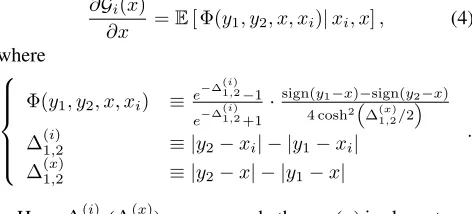
Figure 1:(a)FunctionsGt(x)forc = 1, andxt = −1,0.4, and1. Observations:(i)whenxt =±1, the functionGt(x)is a

monotone function;(ii)for allxt,Gt(x)grows in sublinear manner whenxis close to±1.(b)Definition ofI1, I2andI3used

in the lower bound proof for Lemma 3 (Section 4). Agents inI1andI3are effective anchor agents.(c)Intuition ofE2andE3in

the proof of Lemma 4 (Section 4).

ofxwithout passingy1, y2will not change the probability

that y1 i y2 occurs (i.e., Pr[y1 i y2 | y1, y2, x,E1] =

Pr[y1iy2|y1, y2, x±δ,E1]for any sufficiently smallδ).

Therefore,E1does not impactE[Φ]andE[Φ| E1, x, xi] = 0.

EventE2. Under this event, one can check that|xi−y1|< |xi−y2|(i.e., xi is closer toy1 than toy2). In this case,

when we increase the value ofx(recall thaty1 < x < xi), NK(R{y1,y2}

i , R

{y1,y2}

x )will increase. This is equivalent to

E[Φ| E2, x, xi]>0.

EventE3. Under this event, one can check that|xi−y1|> |xi −y2|.In this case, when we increase the value of x, NK(R{y1,y2}

i , R

{y1,y2}

x )will decrease. This is equivalent to

E[Φ|x, xi,E3]<0.

EventE4.Under this event|xi−y1|−|xi−y2|is positive (we

call this a positive event) with probability 0.5 and is negative (we call this a negative event) with probability 0.5. The first order term conditioned under the positive event cancels out that conditioned under the negative event. Therefore,_E[Φ |

x, xi,E4]will be a “small” term.

With the above intuition, we have

E[Φ|x, xi]≈E[Φ|x, xi,E2] Pr[E2|x, xi] +E[Φ|x, xi,E3] Pr[E3|x, xi].

We now relateE2 andE3 to Example 1. EventE2 corre-sponds to the setting wherexiis closer toy1than toy2. As

explained in Example 1, when we movexto the right, we

increasethe expected KT distance, whereas inE3when we movexto the right, wedecreasethe expected KT distance. The crucial observation is that E2 is much more likely to happen thanE3. The observation becomes clear with

visu-alization in Fig. 3b (i.e., the area forE2is much larger than that forE3). Using these intuitions, we have (see Appendix

B.2 for the full analysis):

Fact 1. Using notations above, we have ,

E[Φ|x, xi] =

X

t=2,3,4

E[Φ|x, xi,Et] Pr[Et|x, xi]>0.

This completes the proof of Lemma 2.

4

Anchor-based nearest neighbor algorithms

for each agentiso that|F~i−F~j|is small if and only ifxi

andxjare close. We present the positive results in the most

general form in 1-dim latent space (i.e., we allow DX and DY to be any near-uniform distribution,p= o(1), and the

latent space is[−c, c]for any constantc).

Index convention. This section usesi, j, and t to index agents and`(include`1,`2, etc.) to index alternatives.

Intuition of the design of F~i. Our key idea is to

lever-age a third lever-agent, namely an anchor agent, to determine the closeness of two agents xi and xj. Let xt be a third

agent. ComputeNK(Rt, Ri)andNK(Rt, Rj). If xt were

chosen appropriately, then NK(Rt, Ri) ≈ NK(Rt, Rj) if

and only ifxi andxj are close. For example, ifxt = −c,

then NK(Rt, Ri) ≈ Gt(xi) and the function Gt(x) is a

monotone function (see the blue curve in Fig. 1a). We have

Gt(xi)≈ Gt(xj)if and only ifxi≈xj.

We face two key technical challenges:C1.Not all agents can be served as effective anchor agents. For example, when

xt= 0,Gt(x) =Gt(−x), which cannot separatexiandxj

whenxi=−xj.C2.the efficacy of the anchor agent is

sen-sitive toxiandxj. For example, whenxt=−c(see again

Fig. 1a), the function Gt(x) grows in a sub-linear manner

so it is less effective in detecting the closeness ofxi andxj

when they are both close to−c.

To address C1, we use all possible agents as anchor agents. To address C2, we need to develop new probabilistic techniques to analyzeGt(x).

Our features. LetF~i= (Fi,1, Fi,2,· · ·Fi,n), where

Fi,t≡ERi,Rt,Y[NK(Ri, Rt)| X] =Gt(xi).

Then we use the L1-distance between F~i andF~j to

deter-mine whetherxiandxjare close. Define

D(xi, xj)≡ 1 n−2

X

t6∈{i,j}

|Fi,t−Fj,t|. (5)

The summation excludesiandj becausexi andxj

them-selves cannot be used as anchor agents.

Replacing the featuresF~ by estimates. Fi,tis not directly

given so we use the empirical estimate as the plug-in esti-mator. DefineFˆi,t = NK(ROi i, R

Ot

t )and our estimator is ˆ

D(xi, xj) =_n−21 Pt6∈{i,j}|Fˆi,t−Fˆj,t|(see Algorithm 2).

Theorem 2. Consider Algorithm Anchor-kNN under

distance-based random preference model. LetDX andDY

Algorithm 2:Anchor-kNN

1 Input:{RO_jj}_j∈[n],k, and agentxi.

2 Output:kneighbors near agenti. 3 ComputeFˆi,j= NK(ROi i, R

Oj

j )for alli, j∈[n].

4 ComputeDˆ(xi, xj) = _n−21 Pt6=i,j|Fˆi,t−Fˆj,t|.

5 Findj1, j2,· · · , jn−1(∈[n]/{i}) such that

ˆ

D(xi, xj1)≤Dˆ(xi, xj2)· · · ≤Dˆ(xi, xjn−1).

6 ReturnXAnchor-kNN← {j1,· · ·, jk}.

an arbitrary quality parameter so that τ(n) = o(1) ∧

τ(n) = ωn−14

√

lnn. For any xi ∈ [−c, c], any m =

ω_p2ln_·τ34n_(n)·ln

2 ln3_n p2_·τ4_(n)

and any k = o(n·τ2_(n)·

ln−1n), we have

max

x∈Anchor-kNN({RO_jj}j,k,xi)

||x−xi||2≤τ(n)

with high probability. The probability comes from random

X/{xi}, randomY, and random preferences.

Remark. τ(n) cannot be too small because our function

D(xi, xj)cannot measure the distance of two agents well if

they are too close.mneeds to grow whenp(fewer samples) orτ(n)decreases (higher quality requirement), which is in-tuitive.kmeasures the number of numbers an algorithm can find so that their distance is withinτ(n); largerkmeans the algorithm is more powerful.

LetD(xi, xj) = E[D(xi, xj)]. In the remainder of this

section, we analyze the behavior of of_D. The function Dˆ

concentrates atDand can be shown by using simple

Cher-noff bounds (see Appendix C.2 for a complete analysis). Lemma 3. For any near-uniform DX,DY on[−c, c]and

any two agentsxi, xj, we have

c3(c)· ln−1n

· |xi−xj|2≤D(xi, xj)≤ |xi−xj|,

wherec3is a constant that depends only onc.

Upper bound proof for Lemma 3. The upper bound re-quires only a straightforward calculation. Recall thatpi =

pi(y1, y2) = Pr[y1iy2|y1, y2, xi]. We have

D(xi, xj) =Ext

Ey1,y2[(pi−pj)(1−2pt)|xi, xj, xt]

≤Ey1,y2[|pi−pj| |xi, xj]≤ |xi−xj|.

(6)

The last inequality is shown in Fact 6 in Appendix C.1. Lower bound bound proof for Lemma 3. Here we analyze only the case|xi−xj| ≤ 2c−2 lnn. When|xi−xj| > 2c−2 lnn (e.g.,xi andxj are around the boundaries −c

andc, respectively), the result is trivial.

Wlog, assume thatxi< xj. We partition[−c, c]into three

intervals and consider anchor agents in each of these inter-vals. Specifically, define (see also Figure 1(b))

I1≡

h

−c,xi−c 2

i

, I2≡

_xi−_c

2 , xj+c

2

&I3≡

h_xj+c

2 , c

i

.

The agents inI2are “less effective anchors” (C2). We use

trivial bound for terms inI2(|Fi,t−Fj,t| ≥0). Focusing on

I1andI3, we have D(xi, xj)

≥ xi+c 4c·cX

·Ext

Gt(xi)− Gt(xj)

|xt∈I1, xi, xj+

c−xj

4c·cX ·Ext

Gt(xi)− Gt(xj)|xt∈I3, xi, xj.

(7)

Note that xi+c

4c·cX+

c−xj

4c·cX is at least

˜

Ω(1). Now we show that

Ext

Gt(xi)− Gt(xj)

|xt∈I1, xi, xj

is at least in the or-der of|xi−xj|2. The analysis for the other term is similar.

Below is the lemma we need (related to C2):

Lemma 4. For any near-uniformDX,DY on[−c, c]such

that|xi−xj| ≥2c−2 lnnandxt∈I1, we have

|Gt(xi)− Gt(xj)| ≥c4(c)· |xi−xj|2,

wherec4(c) = 1−e −c/4

1+e−c/4 ·

1 96c2_·cosh2_(c)·c2

Y

∈(0, 1 2c).

Proof of Lemma 4. Note that |xi − xj| ≥ 2c − 2 lnn

and xt ∈ I1 imply xj ≥ xi ≥ 2xt + c. Because |Gt(xi)− Gt(xj)| =

Rxj

xi

∂Gt(x)

∂x dx

, we aim to give a bound for∂Gt(x)

∂x . Specifically,

∂Gt(x)

∂x ≥3c4(c)·(c

2_−x2_).

when x ≥ 2xt+c(or equivalently, xt ≤ x−₂c). Re-cycle

the definition ofΦ,∆(₁i_,2), and∆(₁x_,2)used in the analysis of Theorem 1 (see also Appendix A for the notation summary) so that ∂G(_∂xx) =_Ey1<y2[Φ(y1, y2, x, xt)|x, xt]

We partition the positions of{y1, y2}into events (see also

Fig. 1c for a visualization):

• E1: whenx≤y1≤y2ory1≤y2≤x.

• E2: wheny1 ∈ [x−7₈ c,3x−5₈ c] andy2 ≥ x+₂c. We have

Pr[E2|y1< y2]≥ c

2_−x2

16c2_c2

Y .

• E3: when(y1, y2)∈ E/ 1∪ E2. As explained below, we do

not need to explicitly calculatePr[E3|y1≤y2].

We now explain the intuition associated with these events.

EventE1. Becausey1andy2are on the same side ofx, we

haveE[Φ| E1, x, xt] = 0(see also Lemma 2).

EventE2and eventE3. When(y1, y2)∈ E2∪ E3, we have |y1−xt| ≤ |y2−xt|(xtis closer toy1than toy2). This is

because(i)|y2−xt| ≥x−xtwheny2 ≥xandx∈ I1,

and(ii)|y1−xt| ≤ max{xt−c, x−xt} ≤x−xtsince

y1≤xandx≥2xt+c. This conclusion is trivial when the

positions of the points are visualized (Figure 1(c)).

In these events, an increment inxwill result in an incre-ment inGt(x). ThereforeE[Φ| E2∪ E3, x, xt]≥0.

Event E2. Knowing Φcan be arbitrarily close to0 when E2∪ E3 happens. Here, we need also identify an event so thatΦis at least a positive constant. EventE2serves for this

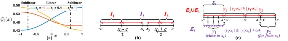
Figure 2: (a)Average pairwise probability prediction error (or pairwise error, see Appendix E.1 for the definition) for different

k∈[101,1601].(b)Pairwise error whenk= 751(optimalkfor ground-truth kNN).(c)The average latent distance betweenxi

and its predicted 751 near neighbors.(d)Validation for high dimension (1∼10dimensional latent space). Letk= 73≈ln2n

and measure the pairwise errors whenk= 73.(e)The average latent distance whenk= 73.

ofy1 andy2, soG(x)behaves like a linear function in this

region (and thus its derivative behaves like a constant). Intuition on dependencies on|xi−xj|2. We now explain

why|Gt(xi)−Gt(xj)|depends on|xi−xj|2instead of|xi−

xj|. Only if(xi, xj)∈ E1/ ,Φwill be non-zero. This requires

y1 ≤ x ≤ y2. Recall we only interests toxi ≤ x ≤ xj.

Whenxiandxjget too close to−c,Pr[y1< x < y2|x] =

Θ(xi+c)≈Θ(|xi−xj|). When we carry out integration

over∂Gt(x)/∂x, this term will lead to an additional factor

of|xi−xj|(see also Figure 1(a) for simulatedGt(x)).

Using the above intuition, we have

Ey1<y2[Φ|x, xt]≥Ey1<y2[Φ| E2, x, xt]·_yPr 1<y2

[E2|x, xt]

= Ω(1)·c

2_−x2

16c2_c2

Y

.

The last inequality uses the fact thatEy1≤y2[Φ| E2, x, xi] = Ω(1)(Fact 7 in Appendix C). By carrying out an integration over∂Gt(x), we get|Gt(xi)− Gt(xj)| ≥c4(c)· |xi−xj|2.

Lemma 4 and its similar result forI3suffice to establish

the lower bound.

5

Experiments

Our experiments aim to (i) confirm the behaviors ofKT

-kNNandAnchor-kNNfor finite sample size whend= 1,

(ii) understand the behavior of Anchor-kNN in high-dim settings, and(iii) validate the practicality of our algorithm over real-world datasets.

Details of all experiments are in Appendix E.1. Note that this is a theoretical paper. Extensive evaluations on real-world data are an promising direction for future work. 1-dim synthetic data. In this experiment we compare the efficacy ofKT-kNN,Anchor-kNN, and Ground-Truth-kNN. Ground-Truth-kNN assumes an oracle access to an input’s (ground-truth)k-nearest neighbors so this is an op-timal kNN. Figure 2(a) plots the performance ofAnchor

-kNN,KT-kNN and Ground-truth-kNN in completing the preferences for different k. Figure 2(b) plots the comple-tion/prediction error for differentxiusing an optimalk

(cho-sen by using cross-validations for Ground-Truth-kNN). Fig-ure 2(c) shows the average latent distance between the return

set andxi. The experiments confirm that(i)Anchor-kNNis

consistently better,(ii)KT-kNNdoes not return near neigh-bors when xi ≈ ±c₂, and(iii) when xi ≈ ±c₂,KT-kNN

is the poorest at completing preferences. Appendix E.1 pro-vides additional experiments for different settings onm. High-dim synthetic data. We repeat the experiments for

d = 1,· · · ,10. Figure 2(d) is the prediction error and Fig-ure 2(e) is the average distance.Anchor-kNNcontinues to outperformKT-kNN, suggesting that our algorithm works ford >1. The performance of all algorithms deteriorate for larged because of the curse-of-dimensionality problem in neighbor-based algorithms (Radovanovi´c, Nanopoulos, and Ivanovi´c 2010).

Real dataset. We examine the performance of Anchor

-kNN using the standard Netflix dataset (Bell and Ko-ren 2007; Bennett, Lanning, and others 2007). The base-lines are KT-kNN and a standard collaborative filtering algorithm using cosine-similarity (Terveen and Hill 2001; Breese, Heckerman, and Kadie 1998). Table 2 in Supple-mentary materials presents the results. Anchor-kNN con-sistently outperforms KT-kNN and collaborative filtering using cosine-similarity. Our experiments suggests that our distance-based random preference model andAnchor-kNN

seem to be quite practical.

6

Conclusion

7

Acknowledgments

We thank all anonymous reviewers for helpful comments and suggestions. AL and LX are supported by NSF #1453542 and ONR #N00014-17-1-2621. QW and ZL are supported by NSF CRII:III #1755769.

References

Abraham, I.; Chechik, S.; Kempe, D.; and Slivkins, A. 2015. Low-distortion inference of latent similarities from a multiplex social network.SIAM Journal on Computing44(3):617–668.

Azari Soufiani, H.; Chen, W.; Parkes, D. C.; and Xia, L. 2013. Gen-eralized method-of-moments for rank aggregation. InAdvances in Neural Information Processing Systems, 2706–2714.

Azari Soufiani, H.; Parkes, D. C.; and Xia, L. 2013. Prefer-ence elicitation for general random utility models. arXiv preprint arXiv:1309.6864.

Azari Soufiani, H.; Parkes, D. C.; and Xia, L. 2014. Computing parametric ranking models via rank-breaking. InICML, 360–368. Bell, R. M., and Koren, Y. 2007. Lessons from the netflix prize challenge.Acm Sigkdd Explorations Newsletter9(2):75–79. Bennett, J.; Lanning, S.; et al. 2007. The netflix prize. In Proceed-ings of KDD cup and workshop, volume 2007, 35. New York, NY, USA.

Breese, J. S.; Heckerman, D.; and Kadie, C. 1998. Empirical anal-ysis of predictive algorithms for collaborative filtering. In Pro-ceedings of the Fourteenth conference on Uncertainty in artificial intelligence, 43–52. Morgan Kaufmann Publishers Inc.

Cheng, W.; H¨ullermeier, E.; and Dembczynski, K. J. 2010. Label ranking methods based on the plackett-luce model. InProceedings of the 27th International Conference on Machine Learning (ICML-10), 215–222.

Fan, C., and Lin, Z. 2013. Collaborative ranking with ranking-based neighborhood. InAsia-Pacific Web Conference, 770–781. Springer.

Hoff, P. D.; Raftery, A. E.; and Handcock, M. S. 2002. Latent space approaches to social network analysis. Journal of the american Statistical association97(460):1090–1098.

Hughes, D.; Hwang, K.; and Xia, L. 2015. Computing optimal bayesian decisions for rank aggregation via mcmc sampling. In UAI, 385–394.

Hwang, S.-w., and Lee, M.-W. 2009. A uncertainty perspective on qualitative preference. InDagstuhl Seminar Proceedings. Schloss Dagstuhl-Leibniz-Zentrum f¨ur Informatik.

Katz-Samuels, J., and Scott, C. 2018. Nonparametric preference completion. InInternational Conference on Artificial Intelligence and Statistics, 632–641.

Khetan, A., and Oh, S. 2016. Data-driven rank breaking for effi-cient rank aggregation.The Journal of Machine Learning Research 17(1):6668–6721.

Kleinberg, J. 2000. The small-world phenomenon: An algorith-mic perspective. InProceedings of the thirty-second annual ACM symposium on Theory of computing, 163–170. ACM.

Liu, T.-Y., et al. 2009. Learning to rank for information retrieval. Foundations and TrendsR in Information Retrieval3(3):225–331.

Liu, N. N., and Yang, Q. 2008. Eigenrank: a ranking-oriented approach to collaborative filtering. InProceedings of the 31st an-nual international ACM SIGIR conference on Research and devel-opment in information retrieval, 83–90. ACM.

Liu, A.; Zhao, Z.; Liao, C.; Lu, P.; and Xia, L. 2019. Learning plackett-luce mixtures from partial preferences. InProceedings of the Thirty-third AAAI Conference on Artificial Intelligence (AAAI-19).

Lu, Y., and Negahban, S. N. 2015. Individualized rank aggregation using nuclear norm regularization. In Communication, Control, and Computing (Allerton), 2015 53rd Annual Allerton Conference on, 1473–1479. IEEE.

Luce, R. D. 1977. The choice axiom after twenty years. Journal of mathematical psychology15(3):215–233.

Maystre, L., and Grossglauser, M. 2015. Fast and accurate infer-ence of plackett–luce models. InAdvances in neural information processing systems, 172–180.

McFadden, D. L. 2000. Economic Choice. Nobel Prize Lecture. Oh, S.; Thekumparampil, K. K.; and Xu, J. 2015. Collaboratively learning preferences from ordinal data. InAdvances in Neural In-formation Processing Systems, 1909–1917.

Park, D.; Neeman, J.; Zhang, J.; Sanghavi, S.; and Dhillon, I. 2015. Preference completion: Large-scale collaborative ranking from pairwise comparisons. InInternational Conference on Ma-chine Learning, 1907–1916.

Plackett, R. L. 1975. The analysis of permutations.Applied Statis-tics193–202.

Radovanovi´c, M.; Nanopoulos, A.; and Ivanovi´c, M. 2010. Hubs in space: Popular nearest neighbors in high-dimensional data.Journal of Machine Learning Research11(2487—2531).

Sarkar, P.; Chakrabarti, D.; and Moore, A. W. 2011. Theo-retical justification of popular link prediction heuristics. In IJ-CAI proceedings-international joint conference on artificial intel-ligence, volume 22, 2722.

Terveen, L., and Hill, W. 2001. Beyond recommender systems: Helping people help each other. HCI in the New Millennium 1(2001):487–509.

Wang, S.; Sun, J.; Gao, B. J.; and Ma, J. 2012. Adapting vector space model to ranking-based collaborative filtering. In Proceed-ings of the 21st ACM international conference on Information and knowledge management, 1487–1491. ACM.

Wang, S.; Sun, J.; Gao, B. J.; and Ma, J. 2014. Vsrank: A novel framework for ranking-based collaborative filtering. ACM Trans-actions on Intelligent Systems and Technology (TIST)5(3):51. Zhao, Z.; Piech, P.; and Xia, L. 2016. Learning mixtures of plackett-luce models. In International Conference on Machine Learning, 2906–2914.