Surface Irrigation Systems

111fiSTER

corr bz

Sur:ace :rrigation Systems'

A. ALVIN BISHOP

Utah State University Logan, Utah

MARVIN E. JENSEN

Agricultural Research Service, USDA Kimberly, Idaho

WARREN A. HALL

University of California Los Angeles, California

I. SURFACE IRRIGATION

In surface irrigation, water is conveyed to the point of infiltration directly on the soil surface. Thus, the soil surface may be considered as the conveyance channel boundary. Surface irrigation channels vary widely in shape, size, and hydraulic characteristics.

The shape of the channel ranges from the small ditches or corrugations used for furrow irrigation of rowcrops, to a wide shallow channel where the entire land surface is flooded. The hydraulic characteristics of the channel may be extremely variable. It may change with time, with the wetting of the soil during an irrigation, and with the growth of the crop between irrigations. Since infiltration occurs, the stream size decreases along this channel and. since the intake rate is not constant, the flow changes with time at a given point in the channel. The hydraulics of surface irrigation systems therefore must account for nonuniform, unsteady flow.

1. ADAPTABILITY

Surface irrigation can be used on nearly all irrigable soils and most crops. The system can be tailored to accommodate a wide range of stream sizes and still maintain a high water application efficiency.

2. FLEXIBILITY

Surface irrigation systems permit ample latitude to meet emergencies. The capacity of most surface systems is sufficient to permit an entire farm to be irri-gated in a small time period as compared to the period between irrigations. The irrigation cycle (period between irrigations), e. g., may be 10 to 14 days whereas the time required to completely irrigate the farm may be only 1 to 3 days. This feature provides an ample factor of safety in case of extreme climatic conditions ' Joint contribution from the Coll. Eng., Utah St. Univ.; the Soil and Water Conserv. Res. Div., ARS, USDA; and the Univ. California.

8 6 6 IRRIGATION SYSTEMS

such as hot drying winds and cloudless days that can cause prolonged periods of high water use by crops. ...he relatively large capacity that can be built into sur-face irrigation systems without additional cost also provides versatility in meeting changing seasonal requirements. If only small continuous flows are delivered to the farm because of water right or water supply restrictions, on-farm storage ponds may be needed to fully utilize this flexibility.

3. ECONOMY

Surface irrigation systems are usually inexpensive to operate when compared with other methods of application because of low power requirements. Water is usually applied directly to the farmland by gravity flow from the irrigation project's canals and laterals. Where water is pumped from wells, rivers, storage reservoirs, or other sources of supply, only enough power to raise the water slightly above the land surface to be irrigated is needed. Labor requirements and costs may be more or less than other methods of irrigation depending on the systems being compared, the manner in which they are operated, the availability of low cost labor, and whether or not automatic controls are used.

4. DEPENDABILITY ,

Surface irrigation is as fully dependable as the water supply. The likelihood of having to interrupt the irrigation for repair of mechanical equipment during periods when crops require large amounts of water is small. Therefore, the poten-tial economic loss due to failure of the system is also small.

A. Types of Systems

Surface irrigation systems may be grouped into two broad classifications, com-plete flooding of the soil surface and partial flooding or furrow method. Comcom-plete flooding which is perhaps the oldest and most widely used method of surface irrigation includes flooding from field ditches, flooding strips between border dikes, and flooding in basins or checks. In this method, the entire land surface in the area being irrigated is covered with water. Water is conveyed to the area in a supply ditch or pipeline, and is distributed over the soil surface in a sheet for the desired time period.

In the partial flooding or furrow method, the entire irrigated area is only partially flooded. Closely spaced furrows (small ditches) contain and distribute the water which moves both laterally and downward from the furrow to moisten the plant root zone.

1. FLOODING FROM FIELD DITCHES

SURFACE IRRIGATION 667

Fig. 43-1. Various methods of applying water to field crops (US Dep. Agr. Farm Se-curity Admin., May 1943).

size of stream, and type and nature of crop. Precise land grading is seldom used

to prepare the land for this method of application. Consequently, both the rate of advance and depth of the water sheet may be extremely variable. Uneven distribution of water and low water application efficiencies are common with uncontrolled flooding from farm ditches.

2. BORDER STRIP FLOODING

The border strip method is a controlled flooding process. The area to be irri-gated is divided into strips or channels by constructing border dikes or levees

(see border irrigation, Fig. 43-1). These dikes restrict the lateral movement of

water, causing it to flow to the end of the field between the dikes. In reality, the border strips are wide, shallow channels in which the water flows from the head ditch to the end of the border strip in an elongating thin sheet, moistening the soil as it goes. This method of irrigation is commonly used when slopes in the direction of irrigation (parallel to the dikes) range from 0.1% to 1.0% for most crops to as much as 6% for pasturelands. When the field slopes in two directions, most of the slope perpendicular to the direction of in-igation (side fall) is eliminated within the border strip by additional land grading so that the advancing sheet covers the entire width of the strip.

8 6 8 IRRIGATION SYSTEMS

rl

On land properly graded, the dikes or levees provide enough control to make this method of irrigation very efficient when properly operated. The dikes should generally be low and rounded on fields with low gradients so that crops can be planted on the dikes as well as on the strip between dikes. In this way no land is taken out of production. Barren dikes may be needed on fields with steeper side slopes and on fine-textured soils to prevent cracking upon drying which could result in lateral movement of the water.

3. BORDER CHECK OR LEVEL BASIN FLOODING

A border check or basin is an area completely surrounded by a dike, Fig. 43-1. The entire desired amount of water is applied quickly and ponded in the area until absorbed by the soil. When properly graded, built to the right dimensions for the soil conditions and size of stream available, and properly operated, checks and basins permit high water application efficiencies and uniform distribution of water.

4. FURROW IRRIGATION

With furrow irrigation small channels or furrows are used to convey the water over the soil surface in small individual, parallel streams, Fig. 43-1. Infiltration occurs through the sides and bottom of the furrow containing water. From the point of infiltration, the water moves both laterally and vertically downward to moisten the plant root zone. The degree of flooding of the land surface depends on the shape, size, and spacing of the furrows, the land slope, and the hydraulic roughness of the furrow.

When crops are grown and cultivated in rows, the construction of furrows between the crop rows can be accomplished as part of the cultivation process. The use of furrows then becomes a natural method for irrigating rowcrops.

Corrugations (small furrows) are often used for irrigating close-growing crops on steep or rolling lands, Fig. 43-1. The corrugations form the major water channels, but some flooding between the corrugations often takes place. This method is especially good for soils that have low intake rates or that disperse when flooded resulting in a hard surface crust upon drying.

869 SURFACE IRRIGATION

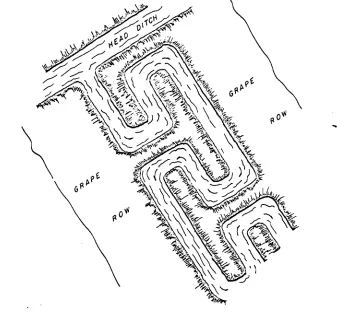
Fig. 43-2. Block system furrow irrigation.

blocked and again diverted to the center furrow and back to the first furrow (see Fig. 43-2).

B. General Characteristics of Surface Irrigation Methods

The adaptations, limitations, and advantages of the various methods of surface irrigation are presented in Table 43-1.

II. DESIGN PRINCIPLES AND PRACTICES

A. Design Principles

The design of a surface irrigation system first involves evaluating the general topographic conditions, soils, crops, farming practices anticipated, and farm operator's desires and finances for the field or farm in question. Information col-lected during the preliminary analysis should be sufficient to permit selecting one

Table 43-1. Adaptations, limitations, and advantages of surface irrigation

Method Adaptation Limitations Advantages

Flooding

From field ditches 1) All irrigable soils 1) Subdivides fields 1) Low initial cost

2) Close growing crops 2) High irrigation labor requirements 2) Adaptable to a wide range Of irrigation flows 3) Slopes up to 10% 3) Low water application efficiency 3) Few permanent structures

4) Rolling lands and shallow soils

where land grading is not feasible 4) Uneven water distribution 4) Runoff from upper areas can he collectedand reused 5) Possible erosion hazard

Border strip 1) All irrigable soils 1) Extensive land grading required I) High water application efficiency possible with good design and operation, regardless of soil type

2) Close growing crops

• 2) Engineering designs necessary forhigh efficiencies 2) Efficient in use of irrigation labor 3) Slopes up to 3% for grains and

forage crops 3) Relatively large flows required 3) Applicable on all soil types 4) Slopes up to 7% for pastures 4) Shallow soils cannot be economically

graded 4) Low maintenance costs

5) Dikes binder cultivation and harvesting 5) Positive control over irrigation water Checks or level 1) All irrigable soils 1) Extensive land grading often required 1) Good control of irrigation water

basins 2) Orchards and close growing crops 2) Large flows required 2) High water application efficiency 3) Slopes up to 24% or more when

benched or terraced 3) Initial cost relatively. high 3) Uniform water applications and leaching 4) Dikes hinder equipment operations 4) Low maintenance costs

5) Maintenance problems on escarpments

on steep slopes 5) Erosion control from irrigation andrainfall 6) May effect crop yields on crops

sensitive to inundation 6) Large streams can be utilized Furrow irrigation

*Corrugations 1) All irrigable soils 1) Moderately high irrigation labor

requirements 1) Increase efficiency and uniformity overflooding from field ditches on rolling lands 2) Slopes up to 10% 2) Short runs required on high intake soils 2) Improves border flooding on new lands 3) Close growing crops 3) Rough on cultivation and harvesting

equipment

Furrow 1) All row crops 1) Moderate irrigation labor requirements 1) Uniform water applications 2) All irrigable soils 2) Engineering design essential for

high efficiencies 2) High water application efficiency 3) Slopes up to 5% with rowcrops

and up to 15% for contour furrows in orchards

3) Some runoff usually necessary for

uniform water application 3) Good control of irrigation water 4) Erosion hazard on steep slopes from

SURFACE IRRIGATION 8 7 1

7. DESIGN DATA

The basic data needed to design a system can be grouped into five general categories:

a. Water. Annual allotment, method of delivery (continuous flow, rotation or demand system, pumped, etc.), stream size available at any time and during peak water use period, quality of irrigation water, expected amount and distribution of rainfall, and irrigation water requirement including leaching requirement.

b. Topography. Major land slopes, field sizes and shapes, uniformity of grades, minor topographic undulations, point of water delivery, and surface

drainage'

characteristics.

c. Soils. Feasibility of constructing canals and ditches without excessive seepage losses, structural stability for canals and ditches, maximum root zone depth, avail-able water-holding capacity, effects of . surface flooding such as crusting and cracking, cumulative intake as a function of time and expected variability be-tween irrigations, erodibility, salt content, and internal drainage capacity.

d. Crops. Types and proportion of each crop to be grown, rooting depths and allowable soil water deficits at various stages of growth, anticipated germination problems, relative sensitivity to inundation, harvesting procedures required, crop rotation systems, and grazing needs.

e. Other. Availability and cost of labor, financial resources available, local customs, degree of maintenance anticipated and maintenance equipment avail-able, and construction equipment available to the operator or through local contractors.

All of the above items have some bearing on the system selected and its final design. Overlooking or neglecting to consider any one of them can impair the effectiveness of the surface method selected.

2. DESIGN OBJECTIVES

A surface irrigation system should be designed rather than merely built in order to assure satisfactory adaption to the soils, topography and crops, and to guarantee uniform irrigations and high water application efficiencies using the available stream size and water supply. Ideally, the system should be capable of repeatedly replenishing the root zone reservoir uniformly before the soil water has been depleted beyond specified limits. The available stream size, and the length and grade of the land units must be combined to achieve these results without excessive labor, waste of water, erosion, and inconvenience to other farming operations.

Designing a system implies that the behavior of performance of the system can be predicted satisfactorily without a trial and error process in the field. If the intake characteristics are known, the designer then predicts two major occur-rences: (i) the advance of the water sheet or furrow flow over the soil surface, and (ii) the recession of this water sheet or furrow flow from the surface.

ESTIMATED OR MEASURED RECESSION CURVE

...-CONTACT TIME

8 7 2 _{122:CATION SYSTZMS}

2

of stream, length of run, and other variables that can be manipulated un-til a satisfactory agreement is reached. a. Advance of the Water. Predict-ing the advance of the water sheet is the most critical of the two items men-tioned and is done by applying known hydraulic principles to overland flow. Field trials are often made to observe the combined influence of crop and ESTIMATED OR MEASURED _{soil roughness, stream size, and} cumu-ADVANCE CURVE

lative intake on the rate of advance. The results of either the predictions or field trials can be plotted, as shown in Fig. 43-3, to evaluate a given combi-nation of variables.

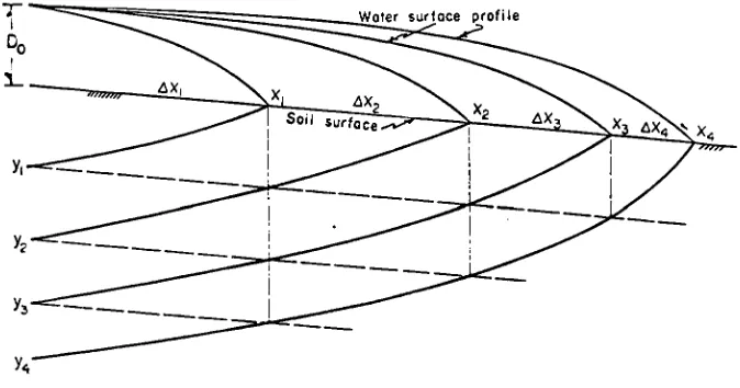
Most investigators have used the continuity equation or water balance equation to predict rate of advance. Hall (1956) used a water balance equation and pre-sented a numerical method for estimating the advance of the sheet of water in a border strip during equal time increments. This method, illustrated in Fig. 43-4,

uses measured cumulative intake as a function of time and assumes a constant

dep: at the upper end of the border strip based on wide channel flow equations. It also assumes that a ratio or shape factor C1 of the volume of surface storage to the volume described by Dox is independent of time, and an additional average depth of water or "puddle factor" E is needed to fill pockets caused by unevenness

of the surface of the border strip. The volume of water on the surface of the soil V. at any time t, is equal to

Vi = w (Car). + c) [43-1]

where

= volume of water on the surface at time to L s ,

w = the width of the border check, L, Do = depth of water at the upper end, L,

E = depth correction factor, L, and x, = distance to leading edge in time to L.

The increment of increased surface storage during any time increment Ati is V, _ _{= [w(Ci Do ± c)][xi – xi} _ i ] = w(Ci Do + c)Axi [43-2]

The volume of intake by the soil is computed in a similar manner except a shape factor, k, is applied only to the last increment of advance, Axi. For other advance increments, the actual intake values based on the measured intake-time relationship are used. When using equal time increments, computation of the average intake depth increment Ayi for an advance increment Axi during time

increment pti reduces to

A Wi = – Yi - 2)/2, > 2. [43-3]

The advance of the water during the first time increment is computed using the DISTANCE , x

SURFACE IRRIGATION 873

Water surface profile

Oo

y4

Fig. 43-4. Cumulative infiltration, y', advance distance, x,, and surface storage after equal time increments, Ati (Hall, 1956).

equation

Ax, =

QAt/w(CiD. +

e kyl) and for

i

2 the advance distances are computed

as

follows

– (Ayi Az/ + Yi AX2 ± • • • + Y2 Axi _ I ) •

—

(C,D.

c +

ky1)

If

D.

is computed from the hydraulic characteristics of the border, the value of will be approximately equal to the tolerance of leveling the field. Severely cracked

soils or a loose, porous surface condition may require much larger values of

if

such conditions were not present during intake measurements. Tabular forms can be used to simplify the recursive computation of Axi.

Less complex approximations of advance distances based on the water balance equation often are justified because hydraulic roughness cannot be predicted accurately and because the intake-time relationship is not constant for different irrigations. These computations are also usually made for a unit width of border strip. One equation used is described below and illustrated graphically

in

Fig.

43-5.

qt = x15 + xy

–

= x(CiDo

C2Y0) [43-6]

where

q = Q/w =

unit stream size or flow per unit width,

(L

a/T) /L = L2 /T,

t =

total time of flow,

T,

x =

distance to the leading edge, L,

= average depth of water on the soil surface, L,

y = average cumulative intake over distance

x,

L,

D.=

depth of water at the upper end, L,

yo = cumulative intake at the upper end, L,

C1 = surface storage coefficient varying from 2/3 to < 1.0, dimensionless, and

C2

=

intake coefficient varying from 0.5 to < 1.0, dimensionless.

[43-4]

874 IRRIGATION SYSTEMS

WATER SURFACE PROFILE

Fig. 43-5. Diagram illustrating the infil-tration-advance problem.

The advance distance at any time t will be

x = qt/ (CiDo C2yo ) [43-7]

The depth of water at the upper end of sloping fields Do rapidly approaches a constant (normal depth). This depth can be computed using one of several open channel flow equations. The value of the C 1 will vary somewhat with the advance distance, slope, and hydraulic characteristics of the border strip, but for practical considerations, it can be assumed to be independent of time. For steep slopes, large advance distances, and small intake rates, C 1 —4 1.0. For flat slopes and small advance distances, and for very high intake rates C 1 —> 0.67. Cumulative intake can be the intake for a soil based on actual measurements, or, for design purposes, cumulative intake can usually be represented adequately by the equa-tion yo = ato° where to is the time water has been on the upper end. The value of C2 will approach 1.0 as b ---> 0 or when cumulative intake approaches a constant. This condition may occur on fine-textured soils that crack severely. After rapid initial intake the rate becomes very slow when the cracks and voids have filled. C2 will approach 0.5 with uniform rate of advance as b --> 1.0 or when slopes are steep so that surface storage is small and cumulative intake is nearly linearly dependent on time. C2 can also be considered independent of time for practical applications.

Analytical solutions for the prediction of advance distance have also been developed. Lewis and Milne (1938) expressed equation [43-7] in differential form essentially as

qt = CiDox +f to y(t - to )e(to )dt, [43-8]

where

t„ = the value of t at which x(t) = s,

y (t - t8 ) = the cumulative infiltration at the point x = s at time t,

(4) = the value of dx/dt at t = t„ and

SURFACE IRRIGATION a 7 5

When cumulative intake can be represented as a function of time, again assuming C1 to be independent of time, analytical solutions to equation [43-8] can be used. Philip and Farrell (1964), using the Laplace transformation, recently pre-sented a detailed derivation of a general solution to the Lewis-Milne infiltration-advance equation. Particular solutions were also presented for the following forms of the cumulative intake function:

y = c [1 – exp (–rt )], y = at ± c [1 – exp (–rt)], y = at', 0 < b < 1, and y = at + ct112 .

Some of the particular solutions require the use of real and complex parameters and the use of the error function (or probability integral). A general description of the use of the error function with tabular values can be found in Carslaw and Jaeger (1959).

Several particular solutions were also expressed in simpler forms for either small t or large t. For example, the particular solution for small t and for the case y = At + Bt112 , where A represents the contribution to infiltration caused by gravity and B the contribution caused by capillary pressure gradient is given below:

For small t and D rB2/16A, where D = CiD„ x= qt 1 _ 2B t

L

3 2 )

For small t and D = B2/16A

B2 – 4Ari t 2 + 7r

8 D . .1. x = r _ 2B ( )1/2 37; B2 (

3 52 32 _{D2 )}

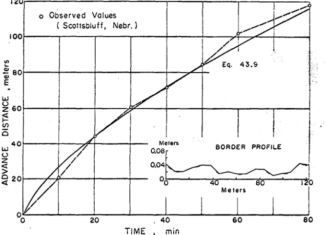
An evaluation of equation [43-9] is illustrated in Fig. 43-6. In this the measured average depth D was used with the cumulative intake in meters and time in minutes, y = 0.00033t + 0.00660/2 . The crop

was alfalfa (Medicago sativa L.), and the border strip was nearly level. Obviously, if the average depth D or CiDo can be predicted from hydraulic properties of the soil and crop, and if the cumulative intake function is known, the advanCe of the water sheet can be readily predicted. Philip and Farrell (1964) also pre-sented a procedure for solving the inverse problem of determining the cumulative intake function using field trial data.

The innumerable variations in soil surface roughness, crop retardance at vari-ous stages of growth, and intake rates from one irrigation to the next have resulted in extensive use of field trials to evaluate the combined effects of the variables on rate of advance. Procedures for conducting field trials are given in other publications (Criddle et al., 1956).

b. Recession of the Water. Procedures for predicting the recession of water from the soil surface have not been sufficiently developed to allow summarization in this chapter. Approximate methods are being used by the Soil Conservation Service, US Department of Agriculture (Shockley et al., 1964). Field trials should be used to check the predicted advance of the water in the border strip or furrow before major irrigation systems are constructed to evaluate the combined effects of the many variables involved. Such field trials can provide sufficient data on recession for design purposes.

8 7 6 IRRIGATION SYSTEMS

o Observed ( Scottsbluff,

Values Nebr.)

0.08 0.04i

..111

Meters

nI

1

-

BORDER PROFILE

11

11did

Fir

Illir

0₀

I

40 Meters

1

80 1 .(

20 40 60 80

TIME , min

Fig. 43-6. Predicted and observed advance distances, and the soil surface profile of the border strip.

L. Designing Flood Irrigation Systems

I. GRADED BOW:a STRIPS

Uniform distribution of water, minimum erosion or other crop and soil damage, high water application efficiency, and economical installation, maintenance and operational costs are commonly the broad objectives in the design of graded border strips. The general topographic requirements of border strip irrigation are relatively fiat or level land of uniform grade and the assurance of good land preparation. Uniformity of irrigation depends on selecting or modifying the variables involved to provide a nearly constant contact time throughout the border strip, Fig. 43-3.

a. Border Strip Slope ,and Size. The slope is largely determined by the existing land slope, or by the amount of topsoil that can be economically and safely removed to obtain the desired slope. Economic considerations can be major fac-tors in determining the final field and border slopes.

By properly matching the intake rate of soil with stream size, area to be irri-gated, depth of water to be applied, and slope of the land, fairly uniform appli-cation can be obtained throughout the border length. Prediction of the rate of advance by one of the methods mentioned previously is a major part of the design of border strips.

Griddle et al. (1956) presented an equation for calculating the contact time necessary using the intake rate equation dy/dt = At". Integration with respect to time gives the cumulative intake, y = (At" 1 ) / (n ± 1). The required con-tact time

t„

necessary to apply the desired depth of irrigation Y becomes

12

100

so E

w Z 60

U)

40 w

CI 20

SURFACE IRRIGATION 8 7 7

e e

g y

li-of

le

ae :et

on-Y(n ± 1)

1,(" • 1)

t

o

=A

L

A

where

t, = required contact time, T,

Y = total depth of water to be applied, L, and n = exponent of t in the intake rate equation.

At the upper end of the border strip, intake begins immediately when water application starts. Intake at the lower end of the field does not begin until some time later depending on the advance time. In order to adequately irrigate the lower end, the total time allotted for applying water must be approximately equal to the contact time required to absorb the desired depth of water plus the advance time.

If the water is in contact with the soil at the lower end of the run just long enough to replenish the soil root zone with the desired quantity of water, deep percolation losses below the root zone can be assumed nil at that point. However, deep percolation losses will occur at all other points in the field, increasing towards the upper end of the border strip, since the actual contact time is greater than the required contact time. The percentage of deep percolation loss will de-pend on the decrease in the intake rate from t = 0 until t = ter for this soil and on the amount of time by which the required contact time is exceeded. By assuming that the deep percolation loss varies uniformly from a maximum at the upper end of the field to zero at the lower end of the field, Bishop (1962) showed that deep percolation loss P, expressed as a percentage of the total water absorbed, could be obtained from the equation

(R + 1)" • 1 – R" • I

P(100) [43-12]

(R 1)** 1

+

• 1

where

P — pc; cent of water intake which is lost by deep percolation below the root

zone,

R = a time ratio = ter/tat where t„ is the required contact time for the desired

depth of irrigation water to be absorbed and to is the advance time, and n = the exponent of t in the intake rate equation previously defined.

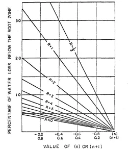
The percentage of loss is plotted against the values of n for different values of R between R = 1/2 to R = 10 in Fig. 43-7. By knowing the intake characteristics of the soil and the value of the exponent n in the intake rate equation the designer

may select a value of R for the deep percolation loss considered allowable. If the allowable deep percolation loss is 6%, for example, the value of R might be as high as 7 for soils with n = –0.1, but a value of R smaller than 0.5 would still be allowable for n = –0.9. The smaller the value of R (larger advance time t0 ), the

longer the allowable length of run for a given soil and stream size. Border strips may be longer with the same percentage of water loss as n approaches –1.0 and shorter as n approaches zero. If the stream can be reduced after the water has advanced to the end of the border strip, thus eliminating any outflow, or when all of the outflow from the border strip is salvaged and used for irrigation on a lower field or recirculated on the same field, deep percolation is the only real

6 7 6 IRRIGATION SYSTEMS

30

20

10

k

liIL

I

1

k11111111

Al

NMI

I I

I I I

.

,

1

R.0

- 0.2 -0.4 -0.6 -0.8 (n)

0.8 0.6 0.4 0.2 (nti)

VALUE OF (n) OR ( n +1 )

Fig. 43-7. Deep percolation—percentage of water lost below the root zone as a function of the cumulative intake parameter n in y at" ", and the ratio, required contact time to advance time, t,r/t. (Bishop, 1962).

loss. Effective irrigation application efficiency then will be related only to the water lost by deep percolation. Under these conditions the water stored in the root zone will be equal to the total quantity applied minus the amount lost through deep percolation. The effective water application efficiency can be esti-mated using either equation [43-12] _{or Fig.} 43-7 _{and the equation:}

E.= 100 – P [43-13]

where

E.= (water stored/water applied) X 100, and

P = the percentage lost by deep percolation obtained from equation [43-12]

or Fig. 43-7.

b. Stream Size. The most desirable size of stream can be determined by evalu-ating the contact times throughout the border strip for various combinations of the variables involved. The stream size available to the farm or field may necessi-tate adjusting the final border strip width to obtain the desired flow per unit width of the border strip.

SURFACE IRRIGATION C 7 9

of curves to be used in estimating the unit-border stream size as a function of intake rate and depth of water to be applied. A unit-border was defined as 100 ft of border strip 1 ft wide. Shockley (1960) presented a modified procedure for estimating the unit-stream for this unit-border that also considers water appli-cation efficiency and the time period before recession begins.

Q. = 1 /

t,

Y

Ea

t, – t,

7.24, where

Q„ =

unit-stream in cubic feet/second,

Ea

=

water application efficiency expressed as a decimal, Y = desired depth of water application in inches,

t„ =

time in minutes required for infiltration of Y inches of water, and

t, = recession

lag time in minutes (from the time the stream is cut off until

re-cession

begins at the upper end).

This equation incorporates increases in the unit-streams to allow for lag in start of --cessi.-.11 on small slopes. Usually the correction is not significant for slopes above 0.5%.

The time required for an irrigation is the time it takes to deliver the volume of water that will provide the desired depth of application, adjusted for the expected efficiency level. The total time

t

in hours can be estimated from equation [43-15] in which the values are

as

previously described, except

t

is now time in hours

t =

Y/432E.Q. [43-15]

where

Y = required net application in inches,

E. =

expected water application efficiency expressed as a fraction,

=

unit-stream in cubic feet/second.

The maximum stream size that can safely be used should also be considered. Criddle et al. (1956) used the following equation to estimate the maximum safe stream in cubic feet per second per foot width of a border strip without sod protection

= 0.06S0.7&

[43-16]

where

q„,„ =

maximum stream in cubic feet per second per foot of width of the bor-der strip, and

S =

slope in per cent.

Criddle (1961) indicates that on slopes less than 0.3% the maximum stream per unit width will be governed by the height of the border dike. With cover crops on these slopes, streams of 0.15 fta/sec per foot of width may result in flow depths of 6 to 8 inches and a stream of 0.2 ft a/sec per foot of width may result in flow depths exceeding 8 inches. Because of difficulties involved in maintaining large dikes, designing for streams less than 0.12 to 0.15 fta/sec per foot of width of the border strip is recommended.

• S C 0 IRRIGATION SYSTEMS

In some cases the minimum flow must also be considered. If the stream size is too small it will not spread laterally across the border strip. The criterion used by Shockley (1960) for the minimum unit stream for graded border irrigation is

q

min

=

0.004S0•5 [43-17]

where

g roin = minimum stream size in cubic foot/sec per foot of border strip width, and

S = slope in per cent.

Lawhon (1960) also developed empirical procedures for designing border strip irrigation systems.

2. LEVEL AND LOW GRADIENT BORDER CHECKS

In level or nearly level border checks and basins the flow is unsteady and nonuniform behind the entire advancing stream. Therefore,

Do

cannot be as-sumed independent of time as with graded border strips. Larger unit streams usually are used and the hydraulic gradients generally are smaller. Thus, more acc,...,ey is required in predicting the volume of surface storage because more of the water remains on the surface during the advance of the water sheet as compared to graded border strips.

The solution of equation [43-7] for border checks requires predicting

Do

as a function of stream size, soil and crop roughness, gradient, and advance distance. Procedures for predicting

Do

as a function of these variables are not . generally available although the hydraulic characteristics of this method of irrigation have been observed in field studies. For example, in a field study at Scottsbluff, Nebraska, USA with alfalfa on a fine sandy loam

Jensen

and Howe (1965) used one stream size, about 4.1 liters/sec per m of width (0.045 ft3 /sec

per

foot of width) and found that the following empirical equation expressed the observed change in depth

D.

as a function of advance distance x: For slopes 0 < S < 0.001 ft/ft and x < 400 ft

Do =

0.175x0.10 – C, [43-18]

where

Do

and x are previously defined and C, = empirical correction for slopes (C, = 300 S – 1500 S 2 ,.0 < S < 0.001). Depth and advance distance dimensions in this case are in feet.

When S 0, equation [43-18] gives the depth

Do

directly for the one stream size, one soil, and one crop. With small gradients, increasing crop retardance materially reduces rate of advance because surface storage is greatly increased. With a dense growth of sugar beets

(Beta vulgaris),

for example, with S = 0.00020, Jensen and Howe (1965) found that the depth

Do

could be represented by

D.=

0.007x0.8 in contrast to

D. =

0.0032.1:0.85 during the first irrigation with little vegetation on a slope of 0.0015. The value of

Do

was nearly doubled as crop retardance increased, thus decreasing the rate of advance of the water sheet. The depth used for the sugar beet data was the average across small furrows and ridges because the water normally overtopped the ridges when retardance was high. The effects of excessive retardance by vegetation can be reduced by main-taining a large open furrow along the border check dikes.

SURFACE IRRIGATION 8 8 1

0.33 of the average total intake time. Thus, the width and length of the border check must be related to the stream size available. Also, the width should be some multiple of the normal rowcrop equipment width to be used.

The depth of irrigation water to be applied will have been fixed by the crop and soil factors previously mentioned. The stream size per unit width will be limited by the width selected and flow available. The length will be limited to the existing field length or some fraction thereof such as one-half, one-third, or one-fourth. Thus, the remaining variable that the designer can adjust freely is the total drop Az or gradient Lz/6,x. Jensen and Howe (1965) derived a

pre-diction equation for estimating the necessary drop to obtain efficient irrigation

Az = ta i/' [43-19]

where

Az = total drop, L,

ta.=advance time or the time for water to reach the end of border check, T, and y' = average intake rate for an irrigation of depth Y, L/T.

This equation also requires predicting the advance of the water sheet. When inadequate data are available for predicting the advance, field trials may be necessary before the design gradient or total drop can be selected. In general when intake rates are extremely small the border checks will be essentially level. When intake rates are large and the contact time is small, the gradient must be increased for the same length of run to compensate for the time required for water to reach the end of the check. More refined surface smoothing to remove low spots may be needed with border checks than with border strips, especially near the lower end of the check.

Other factors to consider in designing border checks or basins are drainage requirements and the effects of inundation on plant growth. In most humid areas, a small gradient and facilities for removing excess water from rainfall are con-sidered essential elements of bench-leveled systems (Phelan, 1960). Some crops

are sensitive to inundation only during warm weather. A large percentage of such crops in a rotation may make the use of border checks undesirable.

Procedures for alignment of benches on steeper lands were given by. Phelan

(1960). Use of border checks is especially advantageous where periodic leaching

is required. Large streams can be used where good water control is available. Also, water control structures can be easily automated.

Crops that must be irrigated after planting to assure germination may necessi-tate combining flat planting beds with deep furrows within the check. This is especially important on soils that develop a dry, hard surface crust after being wetted by flooding.

C. Designing Furrow Irrigation Systems

Furrow irrigation is used for nearly all crops such as corn (Zea mays), potatoes

(Solanum tuberosum), fruit, and vegetables which are grown and cultivated in

Y Li MRICAT:GN SYST2ML

on soils that tend to crust badly after being flooded. Furrow irrigation systems • must be designed to meet crop and cultivation equipment requirements. The maximum furrow slope is fixed by the natural slope of the land or the slope to which the land has been graded. Two other primary factors are: (i) the length of the run, and (ii) the size of the furrow stream. Usually these two factors can be adjusted so as to produce the desired water application efficiency (Bishop, 1962).

I. LEN'Orii OF 12LIN

From a practical viewpoint, furrows should be as long as possible. The longer the furrows, the greater the economy in handling farm equipment and using the irrigator's time. Long furrows reduce the frequency of turning cultivation equip-ment and reduce the number of furrow steam settings.

The same general principles of design as discussed for graded border strips apply to furrow irrigation. The advance time can be estimated or determined by field trials using procedures outlined by Criddle et al. (1956). Davis (1961) developed an equation for predicting advance using the same general relationship Hall (1956) used. The equation for furrows assumes an intake function of the form y, = a (Pt)°, y2 = a (2At)°, etc., and is applicable for i > 2

Fa(At)°

Qat 2 [ay, px1 + Ayi _ 1 6a2 + • . • ± Ay2xi - 2]

[Fa(At)° k CiD.2 j

[43-20] . where F = a factor modifying the intake function because of method of measure-ment. The other variables are as described previously. D o2 is used in place of

D. since furrow volume can be described as a function of D.2 .

Criddle et al. (1956) suggested that the furrow stream should reach the end of the run in one-fourth the required contact time, thus R = 4 for average soil conditions (see graded border strip design). However, as previously mentioned. longer runs would be possible with the same percentage of deep percolation loss

as n approaches -1.0, but shorter runs would be required as n approaches zero.

It is therefore recommended that the value of R used in design should be based on the intake characteristics of the soil to be irrigated (Fig. 43-6).

If runoff from the furrows cannot be salvaged, the size of the runoff stream also plays an important role in the choice of length of run. If the outflow from the furrow for example, amounts to 30% of the inflow stream, then for the aver-age soil conditions assumed by Criddle et al (1956) or n = -0.5, the combined deep percolation plus runoff losses would be about the same for all values of R > 1.0. Under these conditions, the application efficiency would be about 70% and the combined deep percolation and runoff losses would be about 30%. No advantage would be gained by having short irrigation runs (larger values of R), since the reduction in deep percolation loss would be offset by a longer outflow period and greater runoff losses. When runoff is expected, the size of the runoff stream must be evaluated in relation to soil intake characteristics (values of n) and the contact time-advance ratio R.

SURFACE IRRIGATION 883

2. SIZE OF FURROW STRZAM

Once the farm has been prepared for irrigation, i.e. the various fields have been laid out and supply ditches installed, the slope is fixed and the possibilities for altering the spacing and length of furrows becomes limited. Length of furrow can then only be decreased to some fraction of total field length such as one-half, one-third, or one-fourth. The furrow spacing will have been fixed by the farm equipment and crops to be grown. Thus, the furrow stream will be the only variable that can easily be manipulated by the irrigator to achieve adequate and efficient irrigation.

The furrow stream must be large enough to reach the end of the run in the desired time, but small enough to be nonerosive. For most soils, some erosion takes place whenever water flows in the furrow. The larger the stream, the greater the erosion hazard for given conditions. Practical judgment must be used in evaluating the potential erosion problem. What could be considered serious erosion for one farm may be entirely permissible for soil conditions on another. The removal of only 2 to 3 cm (-1 inch) of topsoil from a very shallow soil may be more damaging than erosion of 25 cm or more (1 foot or more) of a deep soil. Criddle (1961) used the following empirical relationship as a guide for determining the maximum allowable furrow streams for various slopes

4, = 10/S [43-21]

where Q, is the maximum nonerosive furrow stream, gallons per minute, and S is slope of the land in per cent. The maximum stream size may also be limited by the capacity of the furrow and the erosion potential by rainfall in some areas may further limit the acceptable slope and length of furrows.

The design of a furrow irrigation system must allow for possible variations in the size of furrow stream because intake rates, advance rates, erodibility, and crop requirements change throughout the irrigation season. Thus, the size of furrow stream must be altered occasionally to offset changes in other variables. By modifying the furrow stream, as required, the irrigator can maintain high water application efficiencies. However, this does not eliminate the need for determining the optimum stream for the initial and adverse conditions. Unfor-tunately with the present status of knowledge, there is no direct method for de-termining the size of stream. Therefore, considerable judgment in the selection of stream size is necessary.

8 3 4 IRRIGATION SYSTZMS

LITERATURE CITED

Bishop, A. A. 1962. Relation of intake rate to length of run in surface irrigation. Amer. Soc. Civ. Eng., Trans. 127:282-293.

Carslaw, H. S., and J. C. Jaeger. 1959. Conduction of heat in solids. 2nd ed. Oxford Univ. Press, London. 510 p.

Criddle, W. D. 1961. Irrigation. McGraw-Hill Book Co. Inc., New York. Agr. Eng. Handbook, Ch. 44, p. 509-531.

Criddle, W. D., S. Davis, C. H. Pair, and D. G. Shockley. 1956. Methods; for evaluating irrigation systems. US Dep. Agr. Handbook No. 82.24 p.

Davis, J. R. 1961. Estimating rate of advalice for irrigation furrows. Amer. Soc. Agr. Eng., Trans. 4(1

):52-54,5:-Hall, W. A. 1956. Estimating irrigation border flow. Agr. Eng. 37(4 ):263-265. Jensen, M. E., and O. W. Howe. 1905. Performance and design of border checks on a

sandy soil. Amer. Soc. Agr. Eng., Trans. 8(1):141-145.

Lawhon, L. F. 1960. Attempts at improvement of design procedures for border irriga-tion. Agr. Res. Serv.-Soil Conserv. Serv. Workshop on Hydraul. of Surface Irrig., Proc. US Dep. Agr.-Agr. Res. Serv. 41-43. p. 7-10.

Lewis, M. R., and W. E. Milne. 1938. Analysis of border irrigation. Agr. Eng. 19:267-268.

Phelan, J. T. 1960. Bench leveling for surface irrigation and erosion control. Amer. Soc. Agr. Eng., Trans. 3(1 ):14-17.

Philip, J. R., and D. A. Farrell. 1964. General solution of the infiltration-advance prob-lem in irrigation hydraulics. J. Geophys. Res. 69(4 ):621-631.

Shockley, D. G. 1960. Present procedures and major problems in border irrigation de-sign. Agr. Res. Serv.-Soil Conserv. Serv. Workshop on Hydraul. of Surface Irrig., Proc. US Dep. Agr.-Agr. Res. Serv. 41-43, p. 1-6

Shockley, Dell G., Hyrum J. Woodward, and John T. Phelan. 1964. A quasi-rational method of border irrigation design. Amer. Soc. Agr. Eng., Trans. 7( 4 ):420-423, 426. US Department of Agriculture Farm Security Administration. 1943. First aid for the