The Thirty-Third AAAI Conference on Artificial Intelligence (AAAI-19)
Word Embedding as Maximum A Posteriori Estimation
∗Shoaib Jameel,
1Zihao Fu,
2Bei Shi,
3Wai Lam,
2Steven Schockaert
4 1School of Computing, Medway Campus, University of Kent, UK2Department of Systems Engineering and Engineering Management, The Chinese University of Hong Kong, Hong Kong 3Tencent AI Lab, Shenzhen, China
4School of Computer Science and Informatics, Cardiff University, UK
[email protected], [email protected], [email protected], [email protected], [email protected]
Abstract
The GloVe word embedding model relies on solving a global optimization problem, which can be reformulated as a max-imum likelihood estimation problem. In this paper, we pro-pose to generalize this approach to word embedding by con-sidering parametrized variants of the GloVe model and in-corporating priors on these parameters. To demonstrate the usefulness of this approach, we consider a word embedding model in which each context word is associated with a cor-responding variance, intuitively encoding how informative it is. Using our framework, we can then learn these variances together with the resulting word vectors in a unified way. We experimentally show that the resulting word embedding mod-els outperform GloVe, as well as many popular alternatives.
Introduction
Word embedding models learn low-dimensional vector rep-resentation of words based on co-occurrence information obtained from some large text corpus. The aim of such mod-els is to learn representations which capture word similari-ties, analogies, and other lexical relationships. Various word embedding models have already been proposed in the lit-erature, including approaches inspired by neural language models, such as Skipgram (SG) and the Continuous Bag-of-Word (CBOW) model (Mikolov et al. 2013), regression based models, such as the least squares regression model GloVe (Pennington, Socher, and Manning 2014) and the or-dinal regression model from (Jameel and Schockaert 2017) and different kinds of probabilistic models, such as Gaus-sian embeddings (Vilnis and McCallum 2014), a BayeGaus-sian version of Skipgram (Barkan 2017) and an approach using Dirichlet-Multinomial language models (D-GloVe) (Jameel and Schockaert 2016).
Word embeddings play a crucial role in deep learning ap-proaches to natural language processing tasks, as they allow
∗
Experiments in this work were performed using the ICARUS computational facility from Information Services and the School of Computing Hydra Cluster at the University of Kent. The work described in this paper is partially supported by a grant from the Research Grant Council of the Hong Kong Special Administra-tive Region, China (Project Code: 14203414). Steven Schockaert is supported by ERC Starting Grant 637277.
Copyright c2019, Association for the Advancement of Artificial Intelligence (www.aaai.org). All rights reserved.
for a natural way to represent textual input to neural net-works. Word embeddings have similarly transformed related fields such as information retrieval (Zamani and Croft 2017), (Dehghani et al. 2017), (Ensan 2018), knowledge base com-pletion (Yang, Tang, and Cohen 2016), (Wang et al. 2014), (Zhong et al. 2015) and recommender systems (Musto et al. 2015), (Zhao et al. 2017).
The approach we follow in this paper is based on GloVe (Pennington, Socher, and Manning 2014). This model aims to find two vector representations, denoted bywiandw˜i, and two bias terms bi and b˜i for each word i such that wi·w˜j+bi+ ˜bjapproximateslogxij, withxij the number
of times wordsiandjco-occur1that co-occurrence counts are weighted based on how closely together the wordsiand j appear. Given GloVe’s formulation as a least squares re-gression problem, it can be naturally interpreted in terms of maximum likelihood estimation. Specifically, it is easy to see that the basic2 GloVe objective is equivalent to maxi-mizing the following expression:
Y
i,j
N(logxij;wi·w˜j+bi+ ˜bj, σ2) (1)
where we writeN(.;µ, σ2)for the Normal distribution with
mean µ and variance σ2. The variance σ2 encodes how
closely we expectwi·w˜j+bi+ ˜bjto approximatelog(xij).
In GloVe, this variance is assumed to be fixed for every word pair(i, j). In such cases,σ2can be chosen arbitrarily, as the choice ofσ2 does then not affect which word vectors and
bias terms maximize (1). Intuitively, however, it seems de-sirable to use a variance σ2
j which depends on how
infor-mative the context word j is: if j is a highly informative context word, it should have a strong influence on the word vector representation ofiand thus we intuitively want the associated varianceσ2j to be low. On the other hand, ifjis a stop word, we may not want it to influence the word vector representation ofiat all, and thus wantσ2j to be high.
The method we develop in this paper will allow us to learn a suitable varianceσ2j for each context wordj. To this end, we will put priors on these variances, and maximize the re-sulting posterior distribution instead of (1), which will allow
1
As usual, we will assume throughout the paper
2
us to jointly learn the informativeness of each context word and the actual word embedding. More generally, by treating the problem of learning a word embedding as maximum a posteriori (MAP) estimation, rather than a maximum likeli-hood estimation problem, a wide range of parametrized vari-ants of GloVe could be considered.
To the best of our knowledge, the idea of using priors to learn parametrized word embedding models has not yet been considered. However, the importance of priors has been ex-tensively studied in the context of probabilistic topic models (Wallach, Mimno, and McCallum 2009). In particular, the widely used Latent Dirichlet Allocation (LDA) (Blei, Ng, and Jordan 2003) model can be seen as a variant of proba-bilistic Latent Semantic Analysis (pLSA) (Hofmann 1999) which includes priors. In this sense, the relationship between our proposed approach and the GloVe model is somewhat analogous to the difference between LDA and pLSA.
Related Work
Probabilistic Word Embedding Models.While, to the best our knowledge, our MAP based generalization of GloVe has not yet been considered, a number of probabilistic models for generating word embeddings have already been stud-ied. One approach, called Gaussian embeddings, was intro-duced by Vilnis et al. (Vilnis and McCallum 2014) and fur-ther developed in (Chac´on 2016). The main underlying idea is to represent words using Gaussian distributions, with the aim of capturing the diversity of word meaning, although this idea has also been applied in applications such as col-laborative filtering (Dos Santos, Piwowarski, and Gallinari 2017) and knowledge graph embedding (He et al. 2015). In-tuitively, the Gaussian representation of a given wordwcan be viewed as a soft region in the word embedding space, en-coding the kinds of contexts in which the word may appear. One of the main underlying motivations is that such mod-els should be better suited for modelling hypernymy. Note that Gaussians (with diagonal covariance matrices) are used in this approach to compactly represent regions, rather than for capturing uncertainty. Non-probabilistic representations for representing words as regions have been considered as well. For instance, (Jameel and Schockaert 2017) used or-dinal SVM regression with a quadratic kernel to learn word regions. These approaches clearly differ from our work, as we still represent words using vectors, but use a probabilistic formulation to find these vectors.
Bayesian versions of Skipgram have been studied in (Barkan 2017) and (Bravzinskas, Havrylov, and Titov 2016), which respectively rely on standard variational techniques and on variational autoencoders for performing inference. The aim of such approaches is to replace point estimates by distributions of word vectors. While the representation of words as probability distributions is similar as in Gaussian embeddings, the motivation is slightly different: in the latter approach the Gaussian distributions are themselves viewed as representations of the words, whereas the Bayesian mod-els assume that words are represented as vectors, but they model uncertainty about the true vector representations of the words. Still, experiments in (Bravzinskas, Havrylov, and Titov 2016) show that such Bayesian models can be used in
a similar way as Gaussian embeddings, with similar levels of performance. Our work is different in that we are using max-imum a posteriori estimates, rather than aiming to character-ize the full posterior distributions, which means that we can keep our models highly efficient. The motivation of our work is also different: whereas the aforementioned Bayesian Skip-gram models aim at characterizing the uncertainty of word vector representations, our aim is to develop parametrized generalizations of the GloVe model.
Our model is also related to the work of (Jameel and Schockaert 2016), which introduced the idea that variance, in the probabilistic formulation of GloVe, can be related to the informativeness of context words. However, they esti-mate this informativeness in a heuristic way from GloVe embeddings that are initially trained in the standard way. In contrast, our work focuses on the role of priors for jointly learning the parameters of word embedding models and the resulting word vectors, and we use the idea of learning suit-able variances to illustrate the potential of our setting. An-other idea proposed in (Jameel and Schockaert 2016) is to use a Dirichlet-Multinomial language model to smooth co-occurrence counts and to estimate the randomness of these counts, to reduce the impact of infrequent words.
Probabilistic Topic Models.Probabilistic topic models (PTMs) are document representations based on latent vari-ables, which intuitively represent topics. While conceptually different from word embeddings, they have served as an in-spiration for this paper, in particular regarding the impor-tance of priors in such models.
One of the key reasons for using priors in PTMs has been to avoid overfitting. This was motivated by the fact that the pLSA model, which is one of the first PTMs, was found to be prone to overfitting, even when using the tempered EM algorithm (Popescul, Pennock, and Lawrence 2001). In their seminal work, (Blei, Ng, and Jordan 2003) argue that the introduction of priors in their LDA model helps overcome this problem of overfitting. Similarly, in this paper, the in-troduction of priors will allow us to avoid overfitting when considering parametrized variants of the GloVe model.
The use of priors has also made it possible to consider var-ious extensions of the LDA model. Some examples include the use of authorship (Rosen-Zvi et al. 2004), temporal in-formation (Wang, McCallum, and Wei 2007) or class labels (Zhu, Ahmed, and Xing 2012), (Zhu et al. 2014). To the best of our knowledge, similar extensions to word embeddings have not yet been studied, although it is worth mentioning that several hybrid models have been proposed that combine topic and word embedding models (Das, Zaheer, and Dyer 2015), (Li et al. 2016), (Shi et al. 2017).
Model Description
In this section we describe our word embedding model, which is based on Maximum A Posteriori (MAP) estima-tion. From a conceptual point of view, one important differ-ence with GloVe is that we associate a varianceσ2
j with each
wordj, intuitively encoding how strongly the number of co-occurrencesxij of wordsiandjshould influence the word
estimated from the data, i.e. from the co-occurrence statis-ticsxij that are derived from some text corpus. However,
the model will also incorporate a prior over these variances, which intuitively allows us to prevent overfitting.
Let us writeτi for the tuple(wi,w˜i, bi,b˜i), D (the
co-occurrence statistics from) for the given document collection andV for the vocabulary. Our word embedding model has the following general form:
P(m,s,t, ψ|D)∝P(D|m,s)P(m,s|t, ψ)P(t)P(ψ)
where the vectorm= (µ1, ..., µ|V|2)associates a meanµij
with each word pair(i, j),s = (σ21, ..., σ|V2 |)associates a varianceσ2
i with each wordi, andt= (τ1, ..., τ|V|)contains
the usual word embedding parameters. The role ofψwill be explained below. For simplicity, we will assume a uniform prior ontandψ, and thus not consider the probabilitiesP(t)
andP(ψ)in the remainder. The probability P(D|m,s)is evaluated similarly to the maximum likelihood formulation of the GloVe model (1). In particular, we assume that the model defines a Normal distribution for each pair of words
(i, j), which acts as a prediction forlogxij:
P(D|m,s) = Y
i,j xij6=0
N(logxij;µij, σ2j) (2)
where the product ranges over all pairs (i, j) for which xij > 0. Note that differently from the GloVe model, in
our case the meanµij is not directly determined from the
word embedding parameters. Instead, we consider a proba-bility distribution over possible values ofµij, which will be
determined by the parameters of the word embedding model (see below). We refer to the model corresponding to (2) as WeMAP (for “Word Embedding as Maximum A Posteriori estimation”).
We will also consider two variants to (2). First, the GloVe model uses a weighting function f to reduce the impact of rare words. It is defined as f(xij) = (
xij
xmax)
α
if xij ≤ xmax and f(xij) = 1otherwise, where usually
α= 0.75andxmax = 100are chosen. This weighting
func-tion can be taken into account in the probabilistic formula-tion (WeMAP1) as follows:
P(D|m,s) = Y
i,j xij6=0
N(logxij;µij, σ2j)
f(xij) (3)
For the second variant (WeMAP2),logxijis replaced by the
Pointwise Mutual Information (PMI) between occurrences ofiandj. Letθ >0be the smoothing parameter. To esti-mate this PMI, we use Bayesian smoothing as follows:
pmi(i, j) = log
p
ij
pi·pj
pij=
xij+θ
x∗∗+|V|2θ
pi=
xi∗+θ
x∗∗+|V|θ
xi∗=x∗i= X
j∈V
xij x∗∗= X
i,j∈V
xij
This leads to the following variant of (2):
P(D|m,s) =Y
i,j
N(pmi(i, j);µij, σ2j) (4)
One advantage of using this smoothed version of PMI is thatpmi(i, j)is also defined ifxij = 0, which allows us to
consider negative examples. In particular, the product in (4) could, in principle, range over any word pair(i, j), regard-less of whetherxij = 0. In practice, the resulting quadratic
time complexity would be prohibitive, hence we limit the number of pairs for whichxij = 0to a small sample,
sim-ilar to how negative samples are used in e.g. the Skipgram model (Mikolov et al. 2013). In our experiments with this variant, for eachj, we set the numberNjof negative
exam-ples (i.e. the number of randomly sampled wordsifor which xij= 0) asNj= 2· |{i|xij6= 0}|.
The probabilityP(m,s|t, ψ)acts as a prior on the means inmand variances ins. It is defined using the Normal In-verse Gamma (NIG) distribution, which is the usual conju-gate prior for the normal distribution (Murphy 2007). This is a probability distribution over pairs(µ, σ2), which is de-fined as the product of a Normal distribution and an In-verse Gamma (IG) distribution. In particular, we evaluate P(m,s|t, ψ)as follows3:
P(m,s|t, ψ) = Y
i,j xij6=0
NIG(µij, σj2;µ 0
ij, λ, α, β) (5)
The NIG distributions in (5) have four parameters. The pa-rameter µ0ij defines our prior belief about the mean. This key parameter is where the parameters of the actual word embedding come into play:
µ0ij=wi·w˜j+bi+ ˜bj
The parametersαandβare respectively the shape and scale parameters of the Inverse Gamma distribution, and λ is a precision parameter which controls how muchµij can
de-viate from our prior belief µ0
ij. Rather than treating these
parameters as encoding our prior beliefs, as in typical prob-abilistic models, we will assume that these parameters α, β andλare encoded in the vectorψ = (α, β, λ). In par-ticular, in our MAP formulation, these parameters will then be chosen such that they maximize the posterior probability P(m,s,t, ψ|D).
Putting everything together, we learn a word embedding model by maximizing the following:
Y
i,j xij6=0
N(logxij;µij, σj2)NIG(µij, σ2j;µ 0
ij, λ, α, β)
Because the NIG distribution is a conjugate prior of the Nor-mal distribution, this expression simplifies to a product of NIG distributions, which will make the computations easier.
3
For the ease of presentation, we will assume that variant (2) or (3) of the likelihood function is used; for variant (4),P(m,s|t, θ)
Note that we do not need to perform any probabilistic in-ference, as we end up with an optimization problem, which we can simply solve using SGD. Compared to Bayesian in-ference methods, this MAP approach has the advantage of being computationally much easier. Interestingly, it was re-cently found in (Mandt, Hoffman, and Blei 2017) that there are also relationships between approximate Bayesian infer-ence and gradient methods.
Experiments
In this section, we present a series of experiments in which we compare our model with popular and recent state-of-the-art word embedding and topic models, all of which can be classified as dimension reduction methods. Topic models such as LDA are an interesting baseline to additionally con-sider in our experiments given the important role they have played in our motivation. Apart from some common intrin-sic evaluation tasks for word embeddings, we also consider three extrinsic evaluation tasks: text classification, document retrieval and named entity recognition (NER).
Methodology
Corpora: We have considered the May 2018 dump of the English Wikipedia. We pre-processed the dump using a pub-licly available script4, which yielded 4.3 billion tokens. Af-ter removing tokens that appear fewer than 500 times in the collection, we ended up with a vocabulary of 117835 distinct tokens. We have lower-cased and removed punctuations. We have considered a symmetric context window size of 10 words, which is a common choice that has been shown to give good results (Pennington, Socher, and Manning 2014).
Intrinsic evaluation tasks:We have considered three stan-dard evaluation tasks for word embedding models. First, we considered three analogy datasets: the Google Word Anal-ogy dataset5, the Microsoft Research Syntactic Analogies Dataset (MSR)6, and the BATS 3.0 dataset7. Second, we considered 14 word similarity datasets8, and finally two out-lier detection datasets9.
We formatted the BATS 3.0 dataset to be similar to the Google and MSR word analogy datasets, so that we can use the same evaluation script for all word analogy experiments10. The BATS 3.0 dataset has 4 superclasses: “Inflectional Morphology (DI)”, “Derivational Morphol-ogy (DM)”, “Encyclopedia Semantics (ES)”, and “Lexico-graphic Semantics (LS)”. Within each superclass there are 10 subclasses consisting of 50 unique word pairs. We com-pute average accuracy for each of these 10 subclasses and report results for the superclass.
4https://github.com/facebookresearch/fastText 5
https://aclweb.org/aclwiki/Analogy (State of the art)
6
https://aclweb.org/aclwiki/Syntactic Analogies (State of the art)
7
http://vsm.blackbird.pw/bats
8https://github.com/mfaruqui/eval-word-vectors 9
http://lcl.uniroma1.it/outlier-detection/ and https://github.com/belph/wiki-sem-500
10
We have made this formatted dataset along with codes which created them available here: https://bit.ly/2J5MtXj
Evaluation results were obtained using publicly avail-able implementations. For instance, word analogy results for the Google dataset were obtained using the code from the GloVe project11, word similarity results were ob-tained using the VSMLib tool12, and outlier detection re-sults were also obtained from available code13. We share our code, pre-processing scripts and datasets online14. We have indexed the word similarity datasets as follows: EN-MC-30 (E1), EN-MEN-TR-3k (E2), EN-MTURK-287 (E3), EN-MTURK-771 (E4), EN-RG-65 (E5), EN-RW-Stanford (E6), EN-SIMLEX-999 (E8), EN-Verb-143 (S8), 353-ALL (E9), 353-REL (E10), EN-WS-353-SIM (E11), EN-YP-130 (E12), SimVerb-3500 (E13), and RareWords15 (E14). For outlier detection, we use O1 to refer to the dataset by (Camacho-Collados and Navigli 2016) and O2 for the WikiSem-500 dataset (Blair, Merhav, and Barry 2016).
Extrinsic evaluation tasks:We have used the benchmark TREC WT2G16dataset for document retrieval which comes with associated TREC topics (queries) and document an-notations. We represent each document and each query as the average of all the words via their corresponding vec-tors. Then, given a query, the similarity can be modeled as cosine similarity between the document vector and the query vector. For document retrieval tasks, the method of only using embeddings is a weak ranker (Mitra et al. 2016), (Nalisnick et al. 2016). Following Mitra et al. (2016), we use a weighted average of the similarities between embed-dings and the Okapi BM25 model (Robertson and Walker 1994). We have used Elasticsearch17 to construct the index and to retrieve the related documents using the default BM25 model (Robertson and Walker 1994).
For document classification, we used the standard Reuters (Reu52 and Reu8), 20Newsgroups (20NG), TechTC30018 (TTC), and WebKB (WKB) collections, which are avail-able online19 in preprocessed form. We also considered two sentence classification datasets from the Text-Top-Model19 project: the Movie Review Polarity dataset (MRP) and the Subjectivity dataset (SUB). For the named entity recognition (NER) task, we have used the CoNLL-2003 English bench-mark dataset20. To generate the document classification re-sults we have used the Text-Top-Model19 project, which has implementations for many text classification algorithms, as well as code for automatic tuning and model selection. In particular, we used the Convolutional Neural Network (CNN) model from Keras for document classification, and the CNN-based model described in (Kim 2014) for sentence
11
https://github.com/stanfordnlp/GloVe
12http://vsm.blackbird.pw/tools 13
http://lcl.uniroma1.it/outlier-detection/
14
https://bit.ly/2J5MtXj
15https://nlp.stanford.edu/ lmthang/morphoNLM/ 16
http://ir.dcs.gla.ac.uk/wiki/Terrier/WT2G
17
https://github.com/elastic/elasticsearch
18http://techtc.cs.technion.ac.il/techtc300/techtc300.html 19
https://github.com/nadbordrozd/text-top-model
20
Table 1: Word analogy results in Accuracy
GSem GSyn Avg. MSR DI DM ES LS
SG 71.58 60.50 65.45 51.71 55.45 13.48 08.78 67.11 CBOW 64.81 47.39 55.17 45.33 50.58 10.11 07.02 76.43 Gauss 66.33 51.67 58.22 41.38 45.17 12.87 07.90 90.32
GloVe 78.85 62.81 69.97 53.04 55.21 14.82 10.56 88.13 D-GloVe 82.34 62.84 71.55 54.47 55.82 13.39 10.22 77.45 MM (L) 78.89 62.86 70.02 53.54 53.79 14.48 09.09 76.91 MM (Q) 80.80 63.49 71.22 54.47 52.20 12.07 10.24 74.73 NWE 78.84 62.76 71.55 54.26 55.04 13.93 09.18 68.02 SV 57.11 39.25 47.22 29.16 47.01 12.01 08.43 60.21 SVD 73.19 50.29 60.51 42.47 54.97 12.07 10.32 67.12 NMF 62.09 31.50 45.16 27.11 43.91 11.69 09.05 52.55 LDA 59.28 38.16 47.59 29.21 43.69 11.45 08.82 51.54 HDP 63.72 36.97 48.91 28.67 45.02 11.56 08.66 55.76 WeMAP 83.50 63.01 72.16 55.08 56.02 14.95 10.61 90.32
WeMAP1 83.50 63.02 72.18 55.08 56.02 14.95 10.62 90.32
WeMAP2 83.52 63.08 72.19 55.08 56.03 14.95 10.62 90.32
classification. For NER we have used the model described in (Chiu and Nichols 2016) with its online implementation21. This model takes word embeddings as input. We used the default settings and trained the model for 50 epochs.
Baseline Models:We compare our method with several popular and strong baseline models: GloVe (Pennington, Socher, and Manning 2014), Skipgram (SG) (Mikolov et al. 2013), Continuous Bag-of-Words (CBOW) (Mikolov et al. 2013), Gaussian word embeddings (Gauss) (Vilnis and McCallum 2014), D-Glove (Jameel and Schockaert 2016), maximum-margin embeddings (MM) (Jameel and Schock-aert 2017), both in their linear (denoted by L) and quadratic (denoted by Q) versions, SemanticVectors (SV)22(Widdows and Ferraro 2008), Singular Value Decomposition (SVD) (Golub and Reinsch 1970), Non-Negative matrix factoriza-tion (NMF) (Lee and Seung 2001), LDA topic models (Blei, Ng, and Jordan 2003), and their non-parametric counter-part called Hierarchical Dirichlet Processes (HDP) (Teh et al. 2005), and finally the Bayesian extension to the SG model proposed in (Barkan 2017) (NWE). Note that SVD and NMF are applied to a PMI-weighted word-word co-occurrence matrix. The topic models LDA and HDP repre-sent topics as probability distributions over words. We then represent a word as a vector containing the probability of that word in each of the topics.
Parameter selection:All models have some free parame-ters that need to be tuned. For datasets that have pre-defined tuning and testing splits, we used these standard splits. For the other datasets, we randomly selected 20% as tuning data, and we report results on the remaining 80%. The num-ber of dimensions for each model was selected from {50, 100, 300, 400}. For CBOW and SG, we chose the num-ber of negative samples from a pool of{1, 5, 10, 15}. For GloVe, we selected thexmaxvalue from{10, 50, 100}andα from{0.1, 0.25, 0.5, 0.75, 1}. For the Gaussian word
em-21
https://github.com/kamalkraj/
Named-Entity-Recognition-with-\\Bidirectional-LSTM-CNNs
22
https://github.com/semanticvectors/semanticvectors/wiki
bedding approach, we used the spherical Gaussians with KL-divergence, which gave better results than the diago-nal model in our experiments. For D-GloVe, we selected the Dirichlet prior constant from{0.0001, 0.001, 0.01, 0.1, 1000, 2000, 5000, 8000}. For WeMAP2, we selectedθfrom
{0.1, 0.01, 0.001, 0.0001, 0.00001, 0.000001}. The number of iterations for all word embedding models was fixed to 20 and the number of posterior inference iterations for all topic models was fixed to 1000. We have also experimented with the different number of iterations for different models, and in each case we found that no major changes occurred after 20 iterations for the word embedding models and 1000 itera-tions for the topic models. We also experimented with differ-ent learning rate parameters, namely{0.01, 0.001, 0.0001, 0.00001}. For the variational inference-based LDA model, we began with the default hyper-prior values hard-coded in the implementation23, which were later updated after each iteration by the sampler, and we did same for the HDP24 model. Note that parameter selection was done for all tasks, both for the baselines and for the proposed models. The only hyperparameters of WeMAP that need to be tuned are the number of dimensions and the learning rate for SGD. In par-ticular, WeMAP requires less tuning than Skip-Gram (where the parameters of the negative sampling strategy need to be tuned) and GloVe (where the parameters of thef(xij)
weighting function need to be tuned). WeMAP1 uses the f(xij)function from GloVe and thus shares the same
hy-perparameters as GloVe. We have found that 0.75 for alpha andxmax = 100gave us good results most of the time for
WeMAP1 which is also true for GloVe. For WeMAP2 we also need to tune a smoothing parameter, and most of the timeθ = 0.00001gave good results. In our three models, a learning rate of 0.001 consistently gave good results. We have also observed that 300 dimensions almost always led to the best results.
23
http://www.cs.columbia.edu/blei/lda-c/
24
Table 2: Word similarity results in Spearman’sρ
E1 E2 E3 E4 E5 E6 E7 E8 E9 E10 E11 E12 E13 E14 Avg.
SG 0.741 0.742 0.651 0.653 0.757 0.470 0.356 0.289 0.662 0.643 0.726 0.565 0.195 0.470 0.566 CBOW 0.727 0.615 0.637 0.555 0.639 0.419 0.279 0.307 0.618 0.563 0.682 0.227 0.168 0.419 0.490 Gauss 0.632 0.710 0.650 0.620 0.695 0.436 0.283 0.273 0.624 0.601 0.690 0.510 0.147 0.436 0.522 GloVe 0.739 0.746 0.648 0.651 0.752 0.473 0.347 0.308 0.675 0.659 0.732 0.582 0.184 0.422 0.566 D-GloVe 0.750 0.746 0.652 0.659 0.779 0.474 0.347 0.315 0.677 0.659 0.735 0.579 0.188 0.473 0.574 MM (L) 0.740 0.737 0.656 0.651 0.764 0.465 0.339 0.296 0.663 0.649 0.726 0.554 0.186 0.465 0.564 MM (Q) 0.770 0.742 0.649 0.658 0.779 0.480 0.356 0.289 0.688 0.672 0.751 0.565 0.196 0.470 0.576 NWE 0.745 0.677 0.627 0.585 0.737 0.450 0.360 0.334 0.681 0.638 0.749 0.487 0.212 0.450 0.552 SV 0.653 0.671 0.632 0.599 0.591 0.393 0.245 0.276 0.582 0.555 0.672 0.421 0.127 0.393 0.486 SVD 0.606 0.697 0.644 0.620 0.674 0.427 0.279 0.246 0.605 0.596 0.676 0.502 0.141 0.427 0.510 NMF 0.589 0.617 0.618 0.568 0.537 0.324 0.228 0.290 0.537 0.525 0.615 0.372 0.106 0.324 0.446 LDA 0.643 0.657 0.630 0.595 0.592 0.376 0.242 0.261 0.569 0.558 0.655 0.413 0.122 0.376 0.478 HDP 0.632 0.646 0.627 0.584 0.571 0.358 0.234 0.274 0.563 0.548 0.648 0.421 0.113 0.358 0.470 WeMAP 0.764 0.751 0.651 0.657 0.777 0.470 0.361 0.303 0.682 0.663 0.746 0.592 0.196 0.480 0.578 WeMAP1 0.766 0.751 0.651 0.657 0.777 0.470 0.361 0.303 0.683 0.663 0.746 0.592 0.196 0.480 0.578 WeMAP2 0.769 0.752 0.657 0.659 0.779 0.472 0.361 0.303 0.684 0.663 0.748 0.593 0.196 0.480 0.580
Table 3: Outlier detection.
O1 O2
Acc OPP Acc OPP
SG 59.375 90.430 30.466 70.794 CBOW 57.813 89.258 30.645 70.399 Gauss 60.938 90.625 37.957 74.354 GloVe 62.500 91.016 39.677 75.541 D-GloVe 67.188 91.797 39.749 75.555 MM (L) 59.375 89.844 38.530 74.645 MM (Q) 65.625 91.211 38.280 74.881 NWE 62.500 91.406 33.441 71.409 SV 57.813 87.695 29.677 69.951 SVD 57.813 88.281 35.197 72.938 NMF 57.813 87.500 27.814 68.490 LDA 56.250 86.719 28.244 68.242 HDP 59.375 88.281 27.993 68.759 WeMAP 67.188 92.578 39.642 75.720
WeMAP1 64.063 92.188 39.749 75.169 WeMAP2 67.188 92.578 39.677 75.541
Results
Intrinsic Evaluation We first present the results for tradi-tional word embedding tasks. They are summarized in Ta-ble 1 for the analogy datasets, TaTa-ble 2 for the word similar-ity datasets, and Table 3 for the outlier detection datasets. For the analogy datasets, our model clearly and consistently outperforms all of the baselines, with the only exception being the syntactic fragment of the Google dataset, where MM(Q) is marginally better. “Avg.” measures the overall performance on the Google dataset in which WeMAP2 per-forms the best. For outlier detection, our model also achieves the best results, where only D-GloVe is marginally better than some variants of our model on O2 in terms of accuracy. Note that we measure outlier detection performance using Accuracy and Outlier Position Percentage (OPP). The goal of OPP is to reflect the position of the outlier word w.r.t. to
SG
D-GloV e
MM (Q)
GloV e
WeMAPWeMAP1 WeMAP2
10 15 20 25
Figure 1: Run time comparisons with competitive compar-ative methods (CPU hours) for 5 iterations and 300 dimen-sional vectors.
other similar words, where the outlier detection problem is thus evaluated as a ranking problem. These metrics are de-fined in more detail in (Blair, Merhav, and Barry 2016) and (Camacho-Collados and Navigli 2016).
For word similarity, on average our models outperform the baselines, although the improvement is not consistent across all datasets. Note that our model consistently outper-forms the popular SG model. On most datasets, our model also outperforms GloVe and D-GloVe, which are the most closely related models.
We also conducted a running time analysis in CPU hours in Figure 1, where we can see that our model runs faster than most comparative models. This experiment was performed on 3.20 GHz machine with 25 threads.
0.6300 0.6320 0.6340 0.6360 0.6380
Figure 2: Mean Average Precision (MAP) scores on WT2G. In the figure, starting from left, colour refers to SG,
CBOW, Gauss, GloVe, D-GloVe,
MM (L), MM (Q), NWE, SV,
SVD, NMF, LDA, HDP, Okapi
BM25, WeMAP, WeMAP1, and WeMAP2.
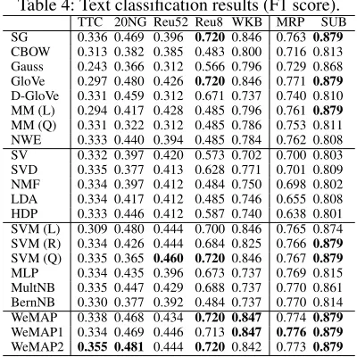
Table 4: Text classification results (F1 score). TTC 20NG Reu52 Reu8 WKB MRP SUB SG 0.336 0.469 0.396 0.720 0.846 0.763 0.879
CBOW 0.313 0.382 0.385 0.483 0.800 0.716 0.813 Gauss 0.243 0.366 0.312 0.566 0.796 0.729 0.868 GloVe 0.297 0.480 0.426 0.720 0.846 0.771 0.879
D-GloVe 0.331 0.459 0.312 0.671 0.737 0.740 0.810 MM (L) 0.294 0.417 0.428 0.485 0.796 0.761 0.879
MM (Q) 0.331 0.322 0.312 0.485 0.786 0.753 0.811 NWE 0.333 0.440 0.394 0.485 0.784 0.762 0.808 SV 0.332 0.397 0.420 0.573 0.702 0.700 0.803 SVD 0.335 0.377 0.413 0.628 0.771 0.701 0.809 NMF 0.334 0.397 0.412 0.484 0.750 0.698 0.802 LDA 0.334 0.417 0.412 0.485 0.746 0.655 0.808 HDP 0.333 0.446 0.412 0.587 0.740 0.638 0.801 SVM (L) 0.309 0.480 0.444 0.700 0.846 0.765 0.874 SVM (R) 0.334 0.426 0.444 0.684 0.825 0.766 0.879
SVM (Q) 0.335 0.365 0.460 0.720 0.846 0.767 0.879
MLP 0.334 0.435 0.396 0.673 0.737 0.769 0.815 MultNB 0.335 0.447 0.429 0.688 0.737 0.770 0.861 BernNB 0.330 0.377 0.392 0.484 0.737 0.770 0.814 WeMAP 0.338 0.468 0.434 0.720 0.847 0.774 0.879
WeMAP1 0.334 0.469 0.446 0.7130.847 0.776 0.879
WeMAP2 0.355 0.481 0.444 0.720 0.842 0.773 0.879
are SVM classifiers which respectively use a linear, RBF and quadratic kernel, MLP is a Multi-layer Perceptron classifier, MultiNB is a Naive Bayes classifier for Multinomial mod-els, and BernNB is a Naive Bayes classifier for multivari-ate Bernoulli models. In document classification task, our model outperforms all baselines, except for the Reuters-52 (Reu52) dataset, where an SVM classifier using the bag-of-words representations achieved the best performance. Note, however, that for this dataset our model is still the best per-forming word embedding model.
On the sentence classification datasets, our model again achieves the best performance (although many models achieve the same performance on SUB). In the NER task, as shown in Table 5, our model performs on par with SG in terms of F1, and it outperforms the other models.
Table 5: NER results showing Precision (Prec.), Recall (Rec.) and F-measure (F1).
Prec. Rec. F1 SG 0.871 0.883 0.877
CBOW 0.853 0.871 0.862 Gauss 0.864 0.880 0.872 GloVe 0.868 0.879 0.874 D-GloVe 0.865 0.877 0.871 MM (L) 0.869 0.879 0.874 MM (Q) 0.862 0.874 0.868 NWE 0.862 0.880 0.874 SV 0.859 0.876 0.867 SVD 0.859 0.873 0.866 NMF 0.844 0.861 0.853 LDA 0.832 0.849 0.840 HDP 0.839 0.856 0.847 WeMAP 0.874 0.878 0.876 WeMAP1 0.876 0.878 0.877
WeMAP2 0.871 0.879 0.875
Conclusions
In this paper, we have introduced a probabilistic word em-bedding model, in which word vectors are learned by find-ing the parameters that maximize a posterior probability. De-spite its probabilistic formulation, our model learns standard word vectors, in contrast to e.g. Bayesian versions of Skip-gram, which aim to learn word representations that take the form of probability distributions. The most immediate prac-tical benefit of our model is the fact that it allows us to asso-ciate a separate variance with each word. In this way, we are able to implicitly take into account the fact that some words are more informative than others. We presented experimen-tal results that showed our model to consistently perform well across a wide range of tasks, while remaining compu-tationally efficient.
The setting we have developed in this paper opens up sev-eral promising avenues for future work. For example, we could straightforwardly extend our model with informed pri-ors on the word vectpri-ors, e.g. to encode prior knowledge from a lexicon. Moreover, the use of priors may allow us to intro-duce additional parameters without overfitting. For exam-ple, in (Jameel and Schockaert 2017) a quadratic regression based word embedding model was found to outperform its linear counterpart. Similarly, we may replace the linear re-gression based formulation of GloVe with a model in which each context word is represented as a quadratic mapping, where priors could be used to encourage the model to stay close to being linear to avoid overfitting in the case of rare context words.
References
Barkan, O. 2017. Bayesian neural word embedding. In AAAI, 3135–3143.
Blei, D. M.; Ng, A. Y.; and Jordan, M. I. 2003. Latent Dirichlet allocation.JMLR3(Jan):993–1022.
Bravzinskas, A.; Havrylov, S.; and Titov, I. 2016. Embedding words as distributions with a Bayesian skip-gram model. NIPS Workshop.
Camacho-Collados, J., and Navigli, R. 2016. Find the word that does not belong: A framework for an intrinsic evaluation of word vector representations. InACL Workshop, 43–50.
Chac´on, E. A. B. 2016. Learning Gaussian word representations with neural networks. Master’s thesis, KU Leuven.
Chiu, J. P., and Nichols, E. 2016. Named entity recognition with bidirectional LSTM-CNNs.TACL4:357–370.
Das, R.; Zaheer, M.; and Dyer, C. 2015. Gaussian LDA for topic models with word embeddings. InACL, 795–804.
Dehghani, M.; Zamani, H.; Severyn, A.; Kamps, J.; and Croft, W. B. 2017. Neural ranking models with weak supervision. In
SIGIR, 65–74. ACM.
Dos Santos, L.; Piwowarski, B.; and Gallinari, P. 2017. Gaussian embeddings for collaborative filtering. InSIGIR, 1065–1068. Ensan, F. 2018. Neural word and entity embeddings for ad hoc retrieval.IPM54(4):657–673.
Golub, G. H., and Reinsch, C. 1970. Singular value decomposition and least squares solutions. Numerische mathematik14(5):403– 420.
He, S.; Liu, K.; Ji, G.; and Zhao, J. 2015. Learning to represent knowledge graphs with gaussian embedding. InCIKM, 623–632. Hofmann, T. 1999. Probabilistic latent semantic analysis. InUAI, 289–296. Morgan Kaufmann Publishers Inc.
Jameel, S., and Schockaert, S. 2016. D-Glove: A feasible least squares model for estimating word embedding densities. In COL-ING, 1849–1860.
Jameel, S., and Schockaert, S. 2017. Modeling context words as regions: An ordinal regression approach to word embedding. In
CoNLL, 123–133.
Kim, Y. 2014. Convolutional neural networks for sentence classi-fication. InEMNLP, 1746–1751.
Lee, D. D., and Seung, H. S. 2001. Algorithms for non-negative matrix factorization. InNIPS, 556–562.
Li, C.; Wang, H.; Zhang, Z.; Sun, A.; and Ma, Z. 2016. Topic modeling for short texts with auxiliary word embeddings. In SI-GIR, 165–174.
Mandt, S.; Hoffman, M. D.; and Blei, D. M. 2017. Stochastic gradient descent as approximate Bayesian inference.JMLR18(1). Mikolov, T.; Sutskever, I.; Chen, K.; Corrado, G. S.; and Dean, J. 2013. Distributed representations of words and phrases and their compositionality. InNIPS, 3111–3119.
Mitra, B.; Nalisnick, E.; Craswell, N.; and Caruana, R. 2016. A dual embedding space model for document ranking.arXiv preprint arXiv:1602.01137.
Murphy, K. P. 2007. Conjugate Bayesian analysis of the Gaussian distribution. Technical Report 2σ2.
Musto, C.; Semeraro, G.; De Gemmis, M.; and Lops, P. 2015. Word embedding techniques for content-based recommender sys-tems: An empirical evaluation. InRecSys Posters.
Nalisnick, E.; Mitra, B.; Craswell, N.; and Caruana, R. 2016. Im-proving document ranking with dual word embeddings. InWWW, 83–84.
Pennington, J.; Socher, R.; and Manning, C. 2014. GloVe: Global vectors for word representation. InEMNLP, 1532–1543.
Popescul, A.; Pennock, D. M.; and Lawrence, S. 2001. Proba-bilistic models for unified collaborative and content-based recom-mendation in sparse-data environments. InUAI, 437–444. Morgan Kaufmann Publishers Inc.
Robertson, S. E., and Walker, S. 1994. Some simple effective approximations to the 2-poisson model for probabilistic weighted retrieval. InSIGIR, 232–241.
Rosen-Zvi, M.; Griffiths, T.; Steyvers, M.; and Smyth, P. 2004. The author-topic model for authors and documents. InUAI, 487–494. Shi, B.; Lam, W.; Jameel, S.; Schockaert, S.; and Lai, K. P. 2017. Jointly learning word embeddings and latent topics. InSIGIR, 375– 384.
Teh, Y. W.; Jordan, M. I.; Beal, M. J.; and Blei, D. M. 2005. Sharing clusters among related groups: Hierarchical dirichlet processes. In
NIPS, 1385–1392.
Vilnis, L., and McCallum, A. 2014. Word representations via Gaus-sian embedding.ICLR.
Wallach, H. M.; Mimno, D. M.; and McCallum, A. 2009. Rethink-ing LDA: Why priors matter. InNIPS, 1973–1981.
Wang, Z.; Zhang, J.; Feng, J.; and Chen, Z. 2014. Knowledge graph and text jointly embedding. InEMNLP, 1591–1601. Wang, X.; McCallum, A.; and Wei, X. 2007. Topical n-grams: Phrase and topic discovery, with an application to information re-trieval. InICDM, 697–702.
Widdows, D., and Ferraro, K. 2008. Semantic vectors: a scalable open source package and online technology management applica-tion. InLREC. Citeseer.
Yang, Z.; Tang, J.; and Cohen, W. W. 2016. Multi-modal Bayesian embeddings for learning social knowledge graphs. InIJCAI, 2287– 2293.
Zamani, H., and Croft, W. B. 2017. Relevance-based word embed-ding. InSIGIR, 505–514. ACM.
Zhao, S.; Zhao, T.; King, I.; and Lyu, M. R. 2017. Geo-teaser: Geo-temporal sequential embedding rank for point-of-interest rec-ommendation. InWWW, 153–162.
Zhong, H.; Zhang, J.; Wang, Z.; Wan, H.; and Chen, Z. 2015. Aligning knowledge and text embeddings by entity descriptions. InEMNLP, 267–272.