A Generalized Language Model in Tensor Space

The Thirty-Third AAAI Conference on Artificial Intelligence (AAAI-19)

A Generalized Language Model in Tensor Space

Lipeng Zhang,

Peng Zhang,

, Xindian Ma,

Shuqin Gu,

Zhan Su,

Dawei Song

2_{School of Computer Science and Technology, Beijing Institute of Technology, Beijing, China} {lpzhang, pzhang, xindianma, shuqingu, suzhan}@tju.edu.cn, [email protected]

Abstract

In the literature, tensors have been effectively used for captur-ing the context information in language models. However, the existing methods usually adopt relatively-low order tensors, which have limited expressive power in modeling language. Developing a higher-order tensor representation is challeng-ing, in terms of deriving an effective solution and showing its generality. In this paper, we propose a language model named Tensor Space Language Model (TSLM), by utiliz-ing tensor networks and tensor decomposition. In TSLM, we build a high-dimensional semantic space constructed by the tensor product of word vectors. Theoretically, we prove that such tensor representation is a generalization of then-gram language model. We further show that this high-order tensor representation can be decomposed to a recursive calculation of conditional probability for language modeling. The exper-imental results on Penn Tree Bank (PTB) dataset and Wiki-Text benchmark demonstrate the effectiveness of TSLM.

Introduction

Language Modeling (LM) is a fundamental research topic that underpins a wide range of Natural Language Process-ing (NLP) tasks, e.g., speech recognition, machine transla-tion, and dialog system (Yu and Deng 2014; Lopez 2008; Wang, Chung, and Seneff 2006). Statistical learning of a language model aims to approximate the probability dis-tribution on the set of expressions in the language (Brown et al. 1992). Recently, Neural networks (NNs), e.g., Recur-rent Neural Networks (RNNs) have been shown effective for modeling language (Bengio et al. 2003; Mikolov et al. 2010; Jozefowicz et al. 2016).

In the literature, a dense tensor is often used to represent a sentence or document. Cai et al. (2006) proposed TensorLSI, which considered sentences or documents as2-order tensors (matrices) and tried to find an optimal basis for the tensor subspace in term of reconstruction error. The 2-order ten-sor (matrix) only reflects the local information (e.g., bi-gram information). Liu et al. (2005) proposed to model text by a multilinear algebraic tensor instead of a vector. Specifi-cally, they represented texts using3-order tensors to capture the context of words. However, they still adopted relatively

∗

Corresponding author: Peng Zhang ([email protected]) Copyright c2019, Association for the Advancement of Artificial Intelligence (www.aaai.org). All rights reserved.

low-order tensors, rather than high-order ones constructed by the tensor product of vectors. For a sentence withnwords (n > 3), an-order tensor (a high-order tensor) constructed by the tensor product of nword vectors, can consider all the combinatorial dependencies among words (not limited to two/three consecutive words in 2/3-order tensor). It turns out that low-order tensors have limited expressive power in modeling language.

It is challenging to construct a high-order tensor based language model (LM), in the sense that it will involve an ex-ponentially increasing number of parameters. Therefore, the research problems are how to derive an effective high-order tensor based LM and how to demonstrate the generality of such a tensor-based LM. To address these problems, our mo-tivation is to explore the expressive ability of tensor space in depth, by making use of tensor networks and tensor decom-position, in the language modeling process.

Tensor network is an elegant mathematical tool and an effective method for solving high-order tensors (e.g., ten-sors in quantum many-body problem), through contractions among lower-order tensors (Pellionisz and Llin´as 1980). Re-cent research shows the connections between neural net-works and tensor netnet-works, which provides a novel per-spective for the interpretation of neural network (Cohen et al. (2016) and Levine et al. (2017; 2018)). With the help of tensor decomposition, the high dimensionality of parame-ters in tensor space can be reduced greatly. Based on tensors, a novel language representation using quantum many-body wave function was also proposed in (Zhang et al. 2018).

Inspired by the recent research, in this paper, we propose a Tensor Space Language Model (TSLM), which is based on high-dimensional semantic space constructed by the ten-sor product of word vectors. Tenten-sor operations (e.g., multi-plication, inner product, decomposition) can be represented intuitively in tensor networks. Then, the probability of a sen-tence will be obtained by the inner product of two tensors, corresponding to the input data and the global parameters, respectively.

con-𝜶𝜶2 𝜶𝜶3 𝜶𝜶𝑛𝑛

𝜶𝜶1 𝑨𝑨

𝒗𝒗 𝑨𝑨 𝒗𝒗

𝒖𝒖

𝑨𝑨 𝛿𝛿 𝑖𝑖 ∈[𝑚𝑚] 𝑑𝑑1∈[𝑚𝑚1]

𝒖𝒖=𝑨𝑨𝒗𝒗

𝑢𝑢𝑖𝑖=� 𝑗𝑗=1 𝑛𝑛

𝐴𝐴𝑖𝑖𝑗𝑗𝑣𝑣𝑗𝑗

𝑑𝑑2∈[𝑚𝑚2]

𝑑𝑑1

𝑑𝑑2

𝑑𝑑3

= (a)

(c) (b)

1) 2) 3) 4)

𝑗𝑗 ∈[𝑛𝑛] 𝑖𝑖 ∈[𝑚𝑚] 𝑖𝑖 ∈[𝑚𝑚]

=

𝑑𝑑1𝑑𝑑2𝑑𝑑3…𝑑𝑑𝑛𝑛

𝓣𝓣

Vector 𝒗𝒗: Matrix 𝑨𝑨: 3-order 𝛿𝛿tensor: 𝑛𝑛-order tensor 𝓣𝓣:

𝑑𝑑1 𝑑𝑑2𝑑𝑑3 …𝑑𝑑𝑛𝑛

𝓣𝓣

𝒔𝒔,𝒄𝒄 = �

𝑑𝑑1,…,𝑑𝑑𝑛𝑛=1 𝑚𝑚

𝒯𝒯𝑑𝑑1…𝑑𝑑𝑛𝑛𝒜𝒜𝑑𝑑1…𝑑𝑑𝑛𝑛

𝑨𝑨=�

𝑖𝑖=1 𝑟𝑟

𝜆𝜆𝑖𝑖𝒖𝒖𝑖𝑖⨂𝒗𝒗𝑖𝑖

(d)

𝛿𝛿

=

𝑼𝑼 𝑖𝑖 𝑖𝑖 𝑽𝑽 𝑗𝑗 𝑘𝑘

𝑘𝑘 𝑗𝑗

𝝀𝝀𝑖𝑖

𝒔𝒔,𝒄𝒄

…

𝑛𝑛-order rank-one tensor 𝓐𝓐: 5)

𝑑𝑑1𝑑𝑑2𝑑𝑑3…𝑑𝑑𝑛𝑛

𝓐𝓐

…

𝜶𝜶1 𝜶𝜶2𝜶𝜶3 … 𝜶𝜶𝑛𝑛

…

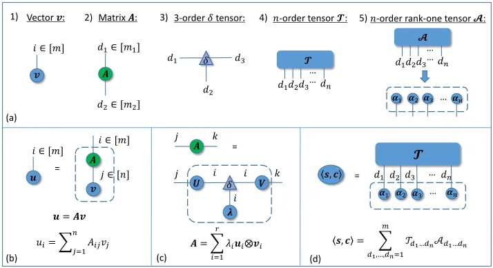
Figure 1: Introduction of Tensor Networks. (a) Tensors in the TN are represented by nodes. (b) A matrixAmultiplying a vector

v in TN notation. The contracted indices are denoted byj and are summed upon. The open indices are denoted byi, their number equals the order of the tensor represented by the entire network. The contraction is marked by the dashed line. (c) A TN notation illustrates the SVD of a matrixA. (d) A TN notation shows the inner product of two tensors.

ditional probability for language modeling. Finally, we eval-uate our model on the PTB dataset and the WikiText bench-mark, and the experimental results demonstrate the effec-tiveness of TSLM.

The main contributions of our work can be summarized as follows: (1) We propose a novel language model aiming to consider high-order dependencies of words via tensors and tensor networks. (2) We prove that TSLM is a generalization of then-gram language model. (3) We can derive a recursive calculation of conditional probability for language modeling via tensor decomposition in TSLM.

Preliminaries

We first briefly introduce tensors and tensor networks.

Tensors

1.Atensorcan be thought as a multidimensional array. The

orderof a tensor is defined to be the number of indexing en-tries in the array, which are referred to as modes. The dimen-sionof a tensor in a particular mode is defined as the num-ber of values that may be taken by the index in that mode. A tensorT ∈ Rm1×···×mn _{means that it is an-order}

ten-sor with dimensionmiin each modei∈[n] :={1, . . . , n}. For simplicity, we also call it amn_{-dimensional tensor in the} following text. A specific entry in a tensor will be referenced with subscripts, e.g.Td1...dn∈R.

2.Tensor productis a fundamental operator in tensor anal-ysis, denoted by⊗, which can map two low-order tensors to a high-order tensor. Similarly, the tensor product of two vector spaces is a high-dimensional tensor space. For exam-ple, tensor product intakes two tensors A ∈ _Rm1×···×mj

(j-order) andB ∈Rmj+1×···×mj+k_{(k-order), and returns a}

tensorA ⊗ B =T ∈ _Rm1×···×mj+k _{((j+k)-order) defined}

by :Td1...dj+k =Ad1...dj · Bdj+1...dj+k.

3.An-order tensorAisrank-oneif it can be written as the tensor product ofnvectors, i.e.,

A=α1⊗α2⊗ · · · ⊗αn (1)

This means that each entry of the tensor is the product of the corresponding vector elements:

Ad1d2...dn=α1,d1α2,d2· · ·αn,dn ∀i, di∈[mi] (2) 4.Therankof a tensorT is defined as the smallest number of rank-one tensors that generateT as their sum (Hitchcock 1927; Kolda and Bader 2009).

Tensor Networks

ATensor Network(TN) is formally represented by an undi-rected and weighted graph. The basic building blocks of a TN are tensors, which are represented by nodes in the net-work. The order of a tensor is equal to the number of edges incident to it. The weight of a edge is equal to the dimension of the corresponding mode of a tensor. Fig. 1 (a) shows five examples for tensors: 1) A vector is a node with one edge. 2) A matrix is a node with two edges. 3) In particular, a triangle node represents aδtensor,δ∈Rm×···×m, which is defined

as follow:

δd1...dn=

1, d1=· · ·=dn

0, otherwise (3)

Edges which connect two nodes in the TN represent a contraction operation between the two corresponding modes. An example for a contraction is depicted in Fig. 1 (b), in which a TN corresponding to the operation of multi-plying a vectorv ∈_Rn_{by a matrixA∈}

Rm×nis performed

by summing over the only contracted indexj. As there is only one open indexi, the result of contracting the network is a vector:u∈Rmwhich upholdsu=Av.

An important concept in the later analysis is Singular Value Decomposition (SVD), which denotes that a matrix

A ∈Rm×ncan be decomposed asA =UΛV, whereΛ ∈ Rr×r represents a diagonal matrix and U ∈ Rm×r, V ∈ Rr×nrepresent orthogonal matrices. In TN notation, we

rep-resent the SVD asA=Pr

i=1λiui⊗viin Fig. 1 (c).λiis a singular value,ui,viare the components ofU,V respec-tively. The effect of theδtensor is shown obviously, which can be observed as ‘forcing’ thei-th ‘row’ of any tensor to be multiplied only by thei-th ‘rows’ of other tensors.

Fig. 1 (d) shows theinner productof two tensorsT and A, which returns a scalar value that is the sum of the prod-ucts of their entries (Kolda and Bader 2009).

Basic Formulation of Language Modeling in

Tensor Space

In this section, we describe the basic formation of Tensor Space Language Model (TSLM), which is used for comput-ing probability for the occurrence of a sequences=wn

1 :=

(w1, . . . , wn)of lengthn, composed of|V|different tokens,

and the vocabularyVcontaining all the words in the model, i.e.wi ∈ V. In the next sections, we will prove that when we use one-hot vectors, TSLM is a generalization ofn-gram language model. If using word embedding vectors, TSLM can result in a recursive calculation of conditional probabil-ity for language modeling. In Related Work, we will discuss the relations and differences between our previous work on language representation for matching sentences (Zhang et al. 2018) and the tensor space language modeling in this paper.

Representations of Words and Sentences

First, we define the semantic space of a single word as a

m-dimensional vector space V with the orthogonal basis

{ed}md=1, where each base vector ed is corresponding to a specific semantic meaning. A wordwi in a sentencescan be written as a linear combination of themorthogonal basis vectors as a general representation:

wi= m

X

di=1

αi,diedi (4)

whereαi,di is its corresponding coefficient. For the basis

vectors{ed}md=1, there can be two different choices, one-hot

vectors or embedded vectors.

As for a sentences= (w1, . . . , wn)with lengthn, it can

be represented in the tensor space:

V⊗n:=V⊗V⊗ · · · ⊗V

| {z }

n

(5)

as:

s=w1⊗ · · · ⊗wn (6)

which is amn-dimensional tensor. Through the interaction of each dimension of words, the sentence tensor has a strong expressive power. Substituting Eq. 4 into Eq. 6, the repre-sentation of the sentencescan be expanded by:

s= m

X

d1,...,dn=1

Ad1...dned1⊗ · · · ⊗edn (7)

where{ed1 ⊗ · · · ⊗edn}

m

d1,...,dn=1 are the basis with m

n

dimension in the tensor space_V⊗n, which denotes the high-dimensional semantic meaning.Ais amn-dimensional ten-sor and its each entryAd1...dn is the corresponding

coeffi-cient of each basis. According to the Eq. 1 and 2, we will seeA, computed asQn

i=1αi,di, is a rank-one tensor.

A Probability Estimation Method of Sentences

A goal of language modeling is to learn the joint probability function of sequences of words in a language (Bengio et al. 2003). We assume that each sentencesiappears with a prob-abilitypi. Then, we can construct a mixed representation c

which is a linear combination of sentences, denoted as:

c:=Xpisi (8)

We consider the mixed representation c as a high-dimensional representation of a sequence containing n

words. For each sentencesi, it can be represented by coeffi-cient tensorAiand basis vectors. Therefore, based on Eqs. 7 and 8, the mixed representationccan be formulated with a coefficient tensorT:

c= m

X

d1,...,dn=1

Td1...dned1⊗. . .⊗edn (9)

The difference betweensin Eq. 7 andcin Eq. 9 is mainly on two different tensorsAandT. According to the Prelim-inaries,Ais essentially rank-one whileT has a higher rank and is harder to solve. We will show that the tensorT en-codes the parameters, andAis the input, in our model.

In turn, if we have estimated such a mixed representation

c(in fact, its coefficient tensorT) from our model, we can get the probabilitypiof a sentencesivia computing the in-ner product ofcandsi:

p(si) =hsi,ci (10)

Based on the Eq. 7, 9 and 10, we can obtain:

p(si) = m

X

d1,...,dn=1

Td1...dnAd1...dn (11)

as shown in the tensor network of Fig 1(d). This is the basic formula in TSLM for estimating the sentence probability.

TSLM as a Generalization of N-Gram

Language Model

𝒉𝒉𝟎𝟎 𝒉𝒉𝟏𝟏 𝒉𝒉𝟐𝟐

𝒙𝒙𝟏𝟏 𝒙𝒙𝟐𝟐

𝒚𝒚𝟏𝟏 𝒚𝒚𝟐𝟐

𝑊𝑊 𝑊𝑊

𝑈𝑈 𝑈𝑈

𝑉𝑉 𝑉𝑉

𝑔𝑔(�,�) 𝑔𝑔(�,�) …

(a)

(b)

𝑈𝑈 𝛿𝛿 𝑊𝑊

𝒉𝒉𝑡𝑡−1

𝜶𝜶𝑡𝑡 = 𝒉𝒉𝑡𝑡

(c) (d)

𝛿𝛿 𝑈𝑈

𝝀𝝀

𝒉𝒉0

𝜶𝜶1 𝜶𝜶2 𝜶𝜶𝑛𝑛

𝓐𝓐 …

…

𝑈𝑈 𝑈𝑈

𝛿𝛿 𝛿𝛿 𝑊𝑊 𝑊𝑊

𝑉𝑉 𝑉𝑉 𝑉𝑉

𝓣𝓣

…

𝒮𝒮(𝑡𝑡−1)

𝑉𝑉

𝛿𝛿

𝑈𝑈

=𝒯𝒯(𝑡𝑡)

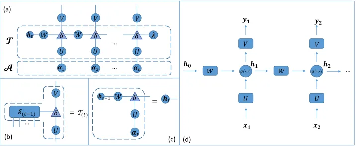
Figure 2: The TN represents the recursive calculation process of TSLM. (a) represents the inner product of two tensorsT and A, (b) denotes the recursive representations ofT(t)and (c) is the recursive representations ofht, respectively. (d) is a general

RNN architecture.

s, its joint probabilityp(s) =p(wn

1) :=p(w1, . . . , wn) re-lies on the Markov Chain Rule of conditional probability:

p(w₁n) =p(w1)

n

Y

i=2

p(wi|w1i−1) (12)

and the conditional probability p(wi|w1i−1) can be

calcu-lated as:

p(wi|w1i−1) = p(wi

1) p(w₁i−1) ≈

count(wi

1)

count(wi−₁ 1) (13)

where thecountdenotes the frequency statistics in corpus.

Claim 1.In our TSLM, when we set the dimension of vec-tor spacem =|V|and each wordwas anone-hotvector, the probability of sentences consist of wordsd1. . . dn in vocabulary is the entryTd1...dnof tensorT.

Proof. The detailed proof can be found in Appendix.

Intuitively, the specific sentencescan be represented as an one-hot tensor. The mixed representationccan be regarded as the total sampling distribution. The tensor inner product hs,cirepresents statistics probability that a sentences ap-pears in a language.

Claim 2.In our TSLM, we define the word sequencewi₁= (w1, w2, . . . , wi)with lengthias:

wi₁:=w1⊗ · · · ⊗wi⊗1i+1⊗ · · · ⊗1n (14) which means that the sequencewi

1is padded via using full

one vector1. Then, the probabilityp(wi1)can be computed

asp(wi

1) =hwi1,ci.

Proof. It can be proved by the marginal probability of

mul-tiple discrete variables (in Appendix).

Therefore, the conditional probability p(wi|wi−1 1) inn

-gram language model can be calculated by Bayesian Condi-tional Probability Formula using tensor representations and tensor inner product as follow:

p(wi|w1i−1) =

hwi

1,ci

hwi−₁ 1,ci (15)

This kind of representation of conditional probability is a special case of TSLM based on the one-hot basis vectors. Because of the one-hot vector representation, the n-gram language model hasO(|V|n_{)parameters. Compared withn} -gram language model, our general model hasO(mn₎ param-eters (m |V|). However, the tensor space still contains exponential parameters, and in the next section, we will in-troduce tensor decomposition to deal with this problem.

Deriving Recursive Language Modeling

Process from TSLM

We have defined the method for estimating probability of a sentencesby the inner product of two tensorsT andAin Eq. 11. In this section, we describe the recursive language modeling process in Fig. 2. Firstly, our derivation is under the condition of basis vectors {ed}md=1 as embedded

vec-tors. Secondly, we recursively decompose the tensorT (see Fig. 3), to obtain the TN representation of tensorT in Fig. 2 (a). Then, we use the intermediate variables in Fig. 2 (bc) to estimate the conditional probability p(wt|w1t−1). In the

following, we introduce the recursive tensor decomposition, followed by the calculation of conditional probability.

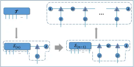
Recursive Tensor Decomposition

We generalize the SVD from matrix to tensor as shown in-tuitively in Fig. 3, inspired by the train-style decomposition of Tensor-Train (Oseledets 2011) and Tucker Decomposi-tion (Kolda and Bader 2009). Fig. 3 illustrates a high-order tensor recursively decomposed as several low-order tensor (vectors, matrices, etc.).

The formula of the recursive decomposition about tensor T is :

T = r

X

i=1

λiS(n),i⊗ui

S(n),k= r

X

i=1

Wk,iS(n−1),i⊗ui

(16)

𝑈𝑈 𝑊𝑊

𝛿𝛿 𝛿𝛿 𝛿𝛿

𝑈𝑈 𝑈𝑈

𝝀𝝀 𝟏𝟏

…

𝓣𝓣

𝑈𝑈 𝛿𝛿 𝝀𝝀 …

𝒮𝒮(𝑛𝑛)

𝑈𝑈 𝛿𝛿 𝝀𝝀 …

𝑊𝑊

𝒮𝒮(𝑛𝑛−1)

𝑈𝑈 𝛿𝛿

Figure 3: The recursive generalized SVD for the tensorT.

tensorT ∈Rm×···×mcan be decomposed as an-order

ten-sor1 _S

(n) ∈ Rm×···×r, a diagonal matrixΛ ∈ Rr×r and a

matrixU ∈Rr×m. One can consider this decomposition as

the matrix SVD after tensor matricization, also as unfold-ing or flattenunfold-ing the tensor to matrix by one mode. Recur-sively, (n-1)-order tensor S(n),k, which can be seen as the

k-th ‘row’ of the tensorS(n), can be decomposed like the

tensorT andWis a matrix composed byrgroups of singu-lar value vectors.

We employ this decomposition to extract the main fea-tures of the tensor T which is similar with the effect of SVD on matrix, then approximately represent the parame-ters of our model, wherer(r≤m) denotes the rank of ten-sor decomposition. This tenten-sor decomposition method re-duce theO(mn_{)magnitude of parameters approximatively} toO(m×r).

A Recursive Calculation of Conditional Probability

In our model, we compute the conditional probability distri-bution as :

p(wt|w1t−1) =sof tmax(hT(t),A(t−1)i) (17)

where A(t−1) is the input of (t-1) words, represented as

α1, . . . ,α(t−1)in Fig. 2 (a).hT(t),A(t−1)iis denoted asyt.

As shown in Fig. 2 (b), T(t) ∈ Rm×···×m×|V| is

con-structed by matrixV ∈ Rr×|V|,S(t−1)and matrixU. The V is the weighted matrix mapping to the vocabulary:

T(t),k= r

X

i=1

Vk,iS(t−1),i⊗ui (18)

As shown in Fig. 2 (c), when calculating the inner prod-uct of two tensorsT andA, we can introduce intermediate variablesht, which can be recursively calculated as:

h1=Wh0Uα1 ...

ht=Wht−1Uαt

(19)

where setting the h0 := W−11, and the matrices W and U decomposed from Eq. 16 in the last section. The

sym-1

To distinguish, we use the first parenthesized subscript to indi-cate the order of the tensor.

boldenotes the element-wise multiplication between vec-tors. This multiplicative operation is derived from the ten-sor product (in Eq. 16) and theδ-tensor, which we have ex-plained it ‘forces’ the two vectors connected with it to be multiplied by elements (in Preliminaries).

Based on the analysis above, the recursive calculation of conditional probability of our TSLM can be formulated as:

p(wt|wt−1 1) =sof tmax(yt)

yt=Vht

ht=g(Wht−1, Uαt) g(a,b) =ab

(20)

whereαt∈Rmis the input at time-stept∈[n],ht∈Rris

the hidden state of the network,yt ∈R|V|denotes the

out-put, and the trainable weight parametersU ∈ Rm×r, W ∈ Rr×r, V ∈Rr×|V|are the input to hidden, hidden to hidden

and hidden to output weights matrices, respectively, andgis a non-linear operation.

The operation stands for element-wise multiplication between vectors, for which the resultant vector upholds(a

b)i=ai·bi. Differently, in the RNN and TSLM architecture,

gis defined as:

g_{RN N}(a,b) =σ(a+b)

g_{T SLM}(a,b) =ab (21)

whereσ(·)is typically a point-wise activation function such as sigmoid, tanh etc. A bias term is usually added to Eq. 21. Since it has no effect with our analysis, we omit it for sim-plicity. We show a general structure of RNN in Fig. 2(d).

In fact, recurrent networks that include the element-wise multiplication operation have been shown to outperform many of the existing RNN models (Sutskever, Martens, and Hinton 2011; Wu et al. 2016). Wu et al. (2016) had given a more general formula for hidden unit in RNN, named Mul-tiplicative Integration, and discussed the different structures of the hidden unit in RNN.

Related Works

Here, we present a brief review of related work, including some representative work in language modeling, and the more recent research on the cross fields of tensor network, neural network and language modeling.

PTB WikiText-2

Train Valid Test Train Valid Test

Articles - - - 600 60 60

Tokens 929,590 73,761 82,431 2,088,628 217,646 245,569

Vocab size 10,000 33,278

OOV rate 4.8% 2.6%

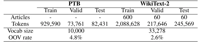
Table 1: Statistics of the PTB and WikiText-2.

PTB WikiText-2

Model Hidden size Layers Valid Test Hidden size Layers Valid Test

KN-5(Mikolov and Zweig 2012) - - - 141.2 - - -

-RNN(Mikolov and Zweig 2012) 300 1 - 124.7 - - -

-LSTM(Zaremba, Sutskever, and Vinyals 2014) 200 2 120.7 114.5 - - -

-LSTM(Grave, Joulin, and Usunier 2016) 1024 1 - 82.3 1024 1 - 99.3

LSTM(Merity et al. 2017) 650 2 84.4 80.6 650 2 108.7 100.9

RNN† 256 1 130.3 124.1 512 1 126.0 120.4

LSTM† 256 1 118.6 110.3 512 1 105.6 101.4

TSLM 256 1 117.2 108.1 512 1 104.9 100.4

RNN+MoS†(Yang et al. 2018) 256 1 88.7 84.3 512 1 85.6 81.8

TSLM+MoS 256 1 86.4 83.6 512 1 83.9 81.0

Table 2: Best perplexity of models on the PTB and WikiText-2 dataset. Models tagged with†indicate that they are reimple-mented by ourselves.

Recently, Cohen et al. (2016) and Levine et al. (2017; 2018) use tensor analysis to explore the expressive power and interpretability of neural networks, including convolu-tional neural network (CNN) and RNN. Levine et al. (2018) even explored the connection between quantum entangle-ment and deep learning. Inspired by their work, Zhang et al. (2018) proposed a Quantum Many-body Wave Function inspired Language Modeling (QMWF-LM) approach. How-ever, in QMWF-LM and TSLM, the term language

mod-elinghas different meanings and application tasks.

Specif-ically, QMWF-LM is basically a language representation

which encodes language features extracted by a CNN, and performs the semantic matching in Question Answer (QA) task as anextrinsic evaluation.

Different from QMWF-LM, in this paper, TSLM focuses on the Markov process of conditional probabilities in lan-guage modeling task with an intrinsic evaluation. Based on the tensor representation and tensor networks, we pro-pose the tensor space language model. We have established the connection between TSLM and neural language models (e.g., RNN based LMs) and proved that TSLM is a more general language model.

Experiments

Datasets

PTBPenn Tree Bank dataset (Marcus, Marcinkiewicz, and Santorini 1993) is often used to evaluate language models. It consists of 929k training words, 73k validation words, 82k test words, and has 10k words in its vocabulary.

WikiText-2 (WT2)dataset (Merity et al. 2017). Compared with the preprocessed version of PTB, WikiText-2 is larger. It also features a larger vocabulary and retains the original case, punctuation and numbers, all of which are removed in PTB. It is composed of full articles.

Table 1 shows statistics of these two datasets. The out of vocabulary (OOV) rate denotes the percentage of tokens have been replaced by anhunkitoken. The token count in-cludes newlines which add to the WikiText-2 dataset.

Evaluation Metrics

Perplexityis the typical measure used for reporting progress in language modeling. It is the average per-word log-probability on the holdout data set.

PPL =e(−n1 P

ilnp(wi))

The lower the perplexity, the more effective the model is. We follow the standard procedure and sum over all the words.

Comparative Models and Experimental Settings

In order to demonstrate the effectiveness of TSLM, we compare our model with several baseline models, in-cluding Kneser-Ney 5-gram (KN-5) (Mikolov and Zweig 2012), RNN based language model (Mikolov et al. 2010), Long Short-Term Memory network (LSTM) based language model (Zaremba, Sutskever, and Vinyals 2014), and RNN added Matrix of Softmax (MoS) language model (Yang et al. 2018). Models tagged with†indicate that they are reim-plemented by ourselves.

Kneser-Ney 5-gram (KN-5): It uses Kneser-Ney Smoothing on then-gram language model (n=5) (Chen and Goodman 1996; Mikolov and Zweig 2012). It is also the most representative statistical language model, and we con-sider it as a low-order tensor language model.

LSTM: LSTM neural network is an another variant of RNN structure. It allows to discover both long and short pat-terns in data and eliminates the problem of vanishing gradi-ent by training RNN. LSTM approved themselves in vari-ous applications and it seems to be very promising course also for the field of language modeling (Soutner and M¨uller 2013).

RNN+MoS: A high-rank RNN language model (Yang et al. 2018) breaking the softmax bottleneck, formulates the next-token probability distribution as a Matrix of Soft-max (MoS), and improves the perplexities on the PTB and WikiText-2. It is the state-of-the-art softmax technique for solving probability distributions.

Since our focus is to show the effectiveness of language modeling in tensor space, we choose to set a relatively small scale network structure. Specifically, we set the same scale parameters for comparison experiments, i.e. 256/512 hid-den size, 1 hidhid-den layer, 20 batch size and 30/40 sequence length. Among them, the hidden size is equivalent to the ten-sor decomposition rankr, and sequence length means the tensor ordernin our model.

Experimental Results and Analysis

Table 2 shows the results on PTB and WT2, respectively. From Table 2, we could observe that our proposed TSLM achieves the lower perplexity, which reflects that TSLM out-perform others. It is obvious that KN-5 method gets the worst performance. We choose KN-5 as a baseline, since it is a typicaln-gram model and we prove that TSLM is a gen-eralization ofn-gram. Although the most advanced Kneser-Ney Smoothing is used, it still has not achieved good perfor-mance. The reason could be that statistic language model is based on the word frequency statistics and does not have the semantic advantages that word vectors in continuous space can satisfy.

The LSTM based language modeling can theoretically model arbitrarily long dependencies. The experimental sults show that our model has achieved relatively better re-sults than LSTM reimplemented by ourselves. Based on the MoS, RNN based language models achieve state-of-the-art results. To prove the effectiveness of our model using MoS, we compared our model to RNN+MoS model on the same parameters. The empirical results of our model have also been improved, which also illustrates the effectiveness of our model structure.

We have shown that TSLM is a generalized language model. In practice, its performance is better than RNN based language model. The reason could be that the non-linear op-erationgin Eq. 20 is an element-wise multiplication, which is capable of expressing more complex semantic informa-tion than a standard RNN structure with activainforma-tion funcinforma-tion using an addition operation.

Note that, the parametersn,mandrare crucial factors for modeling language in TSLM. The order nof the ten-sor reflects the maximum sentence length. With the increase of the maximum sentence length, the performance of the model gradually increases. However, after a certain degree of growth, the expressive ability of the TSLM will reach an upper bound. The reason can be summarized as: The size of

0 10 20 30 40 50 The order n (PTB) 100

110 120 130 140 150 160

PPL

RNN with 256 units LSTM with 256 units TSLM with 256 units

0 10 20 30 40 50 The order n (WikiText-2) 100

110 120 130 140 150 160

RNN with 512 units LSTM with 512 units TSLM with 512 units

Figure 4: Perplexity (PPL) with different max length of sen-tences in corpus.

1632 64 128 256

The rank r (PTB)

100 125 150 175 200 225 250 275 300

PPL

RNN with length 30 LSTM with length 30 TSLM with length 30

3264 128 256 512

The rank r (WikiText-2)

100 125 150 175 200 225 250 275 300

RNN with length 40 LSTM with length 40 TSLM with length 40

Figure 5: Perplexity (PPL) with different hidden sizes.

the corpus determines the size of the tensor space we need to model. The larger the order is, the larger the semantic space that TSLM can model and the more semantic information it can contain. As shown in Fig. 4, we can see that the model is optimal whennequals 30 and 40 on PTB and WikiText datasets, respectively. There are similar experimental phe-nomena in RNN and LSTM.

Other key factors that affect the capability of TSLM are the dimension of the orthogonal basis m and the rank of tensor decomposition r, where each orthogonal basis de-note the basic semantic meaning. The tensor decomposi-tion is enough to extract the main features of the tensor T when r = m. They correspond to the word embedding size and hidden size in RNN or LSTM, and are usually set as the same value. We try to set the value of them as [16,32,64,128,256,512, ...]. As shown in Fig. 5, we can see that the model is optimal when the decomposition rank

requals 256 and 512 on PTB and WikiText datasets, respec-tively. These phenomena is mainly due to the saturation of semantic information in tensor space, which means that the number of the basic semantic meaning is finite with respect to the specific corpus.

Conclusions and Future work

demonstrate the effectiveness of our model, compared with the standard RNN-based language model and LSTM-based language model on two typical datasets to evaluate language modeling. In the future, we will further explore the potential of tensor network for modeling language in both theoretical and empirical directions.

Acknowledgement

This work is supported in part by the state key develop-ment program of China (grant No. 2017YFE0111900), Nat-ural Science Foundation of China (grant No. U1636203, 61772363), and the European Union’s Horizon 2020 research and innovation programme under the Marie Skłodowska-Curie grant agreement No. 721321.

Appendix

Claim 1

In our TSLM, when we set the dimension of vector space

m=|V|and each wordwas anone-hotvector, the proba-bility of sentencesconsist of wordsd1, . . . , dn in vocabu-lary is the entryTd1...dnof tensorT.

Proof of Claim 1

Proof. In our TSLM, when we set the dimension of

vec-tor space m = |V| and each word w as an one-hot vec-tor, the specific sentenceswill be represented as an one-hot tensor. The mixed representationccan be regarded as the total sampling distribution. The tensor inner producths,ci represents statistics probability that a sentencesappears in a language. Specifically, the word wi is an one-hot vector

wi = (0, . . . ,1, . . . ,0), and the vectors of any two different words are orthogonal (word vector itself is basis vector):

hwi,wji=hei,eji=

1, i=j

0, i6=j (22)

Firstly, for the sentences = (w1, . . . , wn)with lengthn is represented ass=w1⊗ · · · ⊗wn. It is an one-hot tensor,

and the tensors of any two different sentences are orthogonal (when being viewed as the flatten vectors):

si=wi,1⊗ · · · ⊗wi,n

sj=wj,1⊗ · · · ⊗wj,n

⇒ hsi,sji= n

Y

k=1

hwi,k,wj,ki

=

1, wi,k =wj,k, ∀k∈[n] 0, otherwise

⇒ hsi,ci=hsi,

X

j

pjsji=pi

(23)

Secondly, for the representations in TSLM, the orthogonal basis can be composed by{wd}|

V|

d=1, and the sentenceswill

be represented as:

s= |V|

X

d1,...,dn=1

Ad1...dnwd1⊗ · · · ⊗wdn (24)

where

Ad1...dn=

1, dk= index(wk,V),∀k∈[n]

0, otherwise (25)

which means tensorAis an one-hot tensor, andindex(w,V) means the index ofwin vocabularyV. We have definedc:=

P

pisias :

c= |V|

X

d1,...,dn=1

Td1...dnwd1⊗ · · · ⊗wdn (26)

Then, the probability of sentencesiis:

pi=hsi,ci

= |V|

X

d1,...,dn=1

Td1...dnAd1...dn

=Td1...dn, dk= index(wk,V),∀k∈[n]

(27)

Therefore, the probability of sentence s consist of words

d1, . . . , dnisp(w1. . . wn=d1. . . dn) =Td1...dn.

Claim 2

In our TSLM, we define the word sequence wi₁ = (w1, w2, . . . , wi)with lengthias:

wi₁:=w1⊗ · · · ⊗wi⊗1i+1⊗ · · · ⊗1n (28) Then, the probabilityp(w₁i)can be computed asp(wi₁) = hwi

1,ci.

Proof of Claim 2

Proof. According to the marginal distribution in probability

theory and statistics, for two discrete random variables, the marginal probability function can be written asp(X=x):

p(X =x) =X

y

p(X =x, Y =y) (29)

wherep(X = x, Y = y)is the joint distribution of two variablesXandY.

Firstly, in our TSLM, we can define the marginal distribu-tion using the word variablewas:

p(wi) =

X

wj∈V

p(wi, wj)

p(w1, . . . , wn−1) = X

wn∈V

p(w1, . . . , wn−1, wn)

(30)

Secondly, the probability of the word sequencewi₁ can be written as:

p(wi₁) =p(w1, . . . , wi)

= X

wi+1,···,wn∈V

p(w1, . . . , wi, wi+1, . . . , wn)

= |V|

X

di+1,···,dn=1

Td1...dn, dk= index(wk,V),∀k∈[i]

Then, the inner producthw1i,cican be written as:

hwi1,ci

=hw1⊗ · · · ⊗1,

|V|

X

d1,···,dn=1

Td1...dnwd1⊗ · · · ⊗wdni

= |V|

X

d1,···,dn=1

Td1...dnhw1⊗ · · · ⊗1,wd1⊗ · · · ⊗wdni

= |V|

X

d1,···,dn=1

Td1...dn

i

Y

j=1

hwj,wdji

n

Y

j=i+1

h1,wdji

= |V|

X

di+1,···,dn=1

Td1...dn, dk= index(wk,V),∀k∈[i]

(32) Therefore, we derive that the probabilityp(wi1)can be

com-puted asp(wi

1) =hwi1,ciaccording to Eq. 31 and 32.

References

Bengio, Y.; Ducharme, R.; Vincent, P.; and Janvin, C. 2003. A neural probabilistic language model. Journal of Machine Learning Research3:1137–1155.

Brown, P. F.; Desouza, P. V.; Mercer, R. L.; Pietra, V. J. D.; and Lai, J. C. 1992. Class-based n -gram models of natural language.Computational Linguistics18(4):467–479.

Cai, D.; He, X.; and Han, J. 2006. Tensor space model for document analysis. InProceedings of the 29th annual inter-national ACM SIGIR conference on Research and development in information retrieval, 625–626. ACM.

Chen, S. F., and Goodman, J. 1996. An empirical study of smoothing techniques for language modeling. InProceedings of the 34th annual meeting on Association for Computational Lin-guistics, 310–318. Association for Computational Linguis-tics.

Cohen, N.; Sharir, O.; and Shashua, A. 2016. On the ex-pressive power of deep learning: A tensor analysis.Computer Science.

Grave, E.; Joulin, A.; and Usunier, N. 2016. Improving neu-ral language models with a continuous cache. arXiv preprint arXiv:1612.04426.

Hitchcock, F. L. 1927. The expression of a tensor or a polyadic as a sum of products.Studies in Applied Mathematics 6(1-4):164-189.

Jozefowicz, R.; Vinyals, O.; Schuster, M.; Shazeer, N.; and Wu, Y. 2016. Exploring the limits of language modeling. arXiv preprint arXiv:1602.02410.

Kneser, R., and Ney, H. 2002. Improved backing-off for m-gram language modeling. In International Conference on Acoustics, Speech, and Signal Processing, 181–184 vol.1. Kolda, T. G., and Bader, B. W. 2009. Tensor decompositions and applications. Siam Review51(3):455–500.

Levine, Y.; Yakira, D.; Cohen, N.; and Shashua, A. 2018. Deep learning and quantum entanglement: Fundamental

connections with implications to network design. In Inter-national Conference on Learning Representations.

Levine, Y.; Sharir, O.; and Shashua, A. 2017. Benefits of depth for long-term memory of recurrent networks. arXiv preprint arXiv:1710.09431.

Liu, N.; Zhang, B.; Yan, J.; and Chen, Z. 2005. Text repre-sentation: from vector to tensor. InIEEE International Confer-ence on Data Mining, 725–728.

Lopez, A. 2008. Statistical machine translation. Acm Com-puting Surveys40(3):1–49.

Marcus, M. P.; Marcinkiewicz, M. A.; and Santorini, B. 1993. Building a large annotated corpus of English: the penn treebank. MIT Press.

Merity, S.; Xiong, C.; Bradbury, J.; Socher, R.; Merity, S.; Xiong, C.; Bradbury, J.; and Socher, R. 2017. Pointer sen-tinel mixture models. InICLR.

Mikolov, T., and Zweig, G. 2012. Context dependent recur-rent neural network language model. SLT12:234–239. Mikolov, T.; Karafi´at, M.; Burget, L.; Cernock´y, J.; and Khu-danpur, S. 2010. Recurrent neural network based lan-guage model. InINTERSPEECH 2010, Conference of the In-ternational Speech Communication Association, Makuhari, Chiba, Japan, September, 1045–1048.

Oseledets, I. V. 2011. Tensor-train decomposition. Siam Journal on Scientific Computing33(5):2295–2317.

Pellionisz, A., and Llin´as, R. 1980. Tensorial approach to the geometry of brain function: Cerebellar coordination via a metric tensor.Neuroscience5(7):1125–1136.

Soutner, D., and M¨uller, L. 2013. Application of lstm neural networks in language modelling. InInternational Conference on Text, Speech and Dialogue, 105–112.

Sutskever, I.; Martens, J.; and Hinton, G. E. 2011. Generat-ing text with recurrent neural networks. InProceedings of the 28th International Conference on Machine Learning (ICML-11), 1017–1024.

Wang, C.; Chung, G.; and Seneff, S. 2006. Automatic induc-tion of language model data for a spoken dialogue system. Language Resources and Evaluation40(1):25–46.

Wu, Y.; Zhang, S.; Zhang, Y.; Bengio, Y.; and Salakhutdi-nov, R. R. 2016. On multiplicative integration with recurrent neural networks. InAdvances in Neural Information Processing Systems, 2856–2864.

Yang, Z.; Dai, Z.; Salakhutdinov, R.; and Cohen, W. W. 2018. Breaking the softmax bottleneck: A high-rank RNN language model. InInternational Conference on Learning Rep-resentations.

Yu, D., and Deng, L. 2014. Automatic Speech Recognition: A Deep Learning Approach. Springer.