Distributed Stochastic Variance Reduced Gradient Methods
by Sampling Extra Data with Replacement
Jason D. Lee [email protected]
Marshall School of Business University of Southern California Los Angeles, CA 90089, USA
Qihang Lin [email protected]
Tippie College of Business University of Iowa
Iowa City, IA 52242, USA
Tengyu Ma [email protected]
Department of Computer Science Princeton University
Princeton, NJ 08544, USA
Tianbao Yang [email protected]
Department of Computer Science University of Iowa
Iowa City, IA 52242, USA
Editor:Francis Bach
Abstract
We study the round complexity of minimizing the average of convex functions under a new setting of distributed optimization where each machine can receive two subsets of functions. The first subset is from a random partition and the second subset is randomly sampled with replacement. Under this setting, we define a broad class of distributed algorithms whose local computation can utilize both subsets and design a distributed stochastic vari-ance reduced gradient method belonging to in this class. When the condition number of the problem is small, our method achieves the optimal parallel runtime, amount of com-munication and rounds of comcom-munication among all distributed first-order methods up to constant factors. When the condition number is relatively large, a lower bound is provided for the number of rounds of communication needed by any algorithm in this class. Then, we present an accelerated version of our method whose the rounds of communication matches the lower bound up to logarithmic terms, which establishes that this accelerated algorithm has the lowest round complexity among all algorithms in our class under this new setting.
Keywords: distributed optimization, communication complexity, first-order method, lower bound, stochastic variance reduced gradient
c
1. Introduction
In this paper, we consider the distributed optimization problem of minimizing the average of N convex functionsfi :Rd→R fori= 1, . . . , N, i.e.,
min
x∈Rd
f(x) := 1 N
N
X
i=1 fi(x)
(1)
using m machines. For simplicity of notation, we assume N =mnfor an integer n but all of our results can be easily generalized for an arbitrary N. In this paper, the norm k · k represents the Euclidean norm and h·,·i represents the inner product in Rd. Throughout the whole paper, we make the following standard assumptions on problem (1).
Assumption 1 The functionsfi for i= 1, . . . , N in (1) satisfy the following properties:
• Each function fi is convex and L-smooth, which means fi is differentiable and its
gradient∇fiisL-Lipschitz continuous, i.e.,k∇fi(x)−∇fi(y)k ≤Lkx−yk, ∀x, y∈Rd.
• The average function f is µ-convex with µ≥0, i.e., f(x)≥f(y) +h∇f(y), x−yi+
µ
2kx−yk
2, ∀x, y∈ Rd.
When µ >0,f isµ-strongly convex and we callκ= Lµ thecondition number off. Note that the functionf itself can beLf-smooth, namely,k∇f(x)−∇f(y)k ≤Lfkx−yk, ∀x, y∈
Rd, for a constantLf ≤L. Letx∗ be an optimal solution of (1) and a deterministic solution
ˆ
x is called an -optimal solution to (1) if f(ˆx) −f(x∗) ≤ . If ˆx is a random variable generated by a stochastic algorithm, we call it an-optimal solution if E[f(ˆx)−f(x∗)]≤. One of the most important applications of problem (1) is empirical risk minimization (ERM) in statistics and machine learning. Let {ξ1, ξ2, . . . , ξN} be a set of i.i.d. samples
from an unknown distribution D. A regularized ERM problem with can be formulated as
min
x∈Rd
f(x) = 1 N
N
X
i=1
φ(x, ξi) +r(x)
, (2)
wherexrepresents a vector of parameters of a predictive model,φ(x, ξ) is a loss function, and r(x) is a regularization term. Note that (2) has the form of (1) withfi(x) =φ(x, ξi) +r(x).
A commonly used regularization term is r(x) = λ2kxk2 and the regularization parameterλ
significantly influences µ and κ. The value of λ is typically in the order of Θ(1/√N) = Θ(1/√mn) as justified by Shamir and Srebro (2014), Shamir et al. (2014), Shalev-Shwartz et al. (2009) and Zhang and Lin (2015). For simplicity, in the rest of the paper, we will call fi theith data point or theith function interchangeably.
We consider a situation where allN functions are initially stored in a large storage space that has limited computation power. Then, these N functions are partitioned, sampled and distributed to m machines where the main computation is performed for solving (1). One common practice under a classical setting is to randomly and evenly partition the N functions into subsets S1, S2, . . . , Sm with|Sj|= Nm =n and storeSj in machinej. In this
paper, we consider a new setting where an extra set of functions Rj with |Rj| ≤ O(|Sj|)
machine j for the local computation. Since no machine can access all N functions, we consider solving (1) by synchronized distributed algorithms that alternate between a local computation procedure at each machine, and a round of communication to share information among the machines.
One contribution of this paper is to develop a distributed algorithm for (1) under this new setting. Compared to the previous methods where onlySjis stored in machinej, our method
requires more storage space or machines but significantly fewer rounds of communication to achieve an -optimal solution for (1) when the problem’s parameters are in a practical regime, showing the advantage of the new setting. Moreover, we define a broad class of distributed algorithms for (1) under the new setting, which includes the proposed method, and establish a lower bound for the number of rounds of communication needed by any algorithm in this class to find an-optimal solution. This lower bound matches the number of rounds required by the proposed method up to logarithmic factors, indicating that our lower bound is tight and the proposed method is nearly optimal in this class.
1.1 Performance Metrics
In the design of distributed algorithms, one often needs to consider more performance met-rics than in the single-machine scenario. A priori, the most important performance metric is the total runtime of algorithm—the time difference between the start of the first machine and the end of the last machine. However, there are other factors than the machines’ CPU time that affect the total runtime such as the communication between machines. Moreover, the latency in initiating communication is also non-negligible, and often the bottleneck of the entire system.
We use the following synchronous message passing model from the distributed compu-tation literature, e.g., Gropp et al. (1996) and Dean and Ghemawat (2008): We assume the communication occurs in rounds—in each round, machines exchanges messages with each other and, between two rounds, machines only perform computation based on their local information (local data points and messages received before). Under this model, three metrics are of main interests to us:
• Parallel runtime: The longest running time of themmachines spent in local parallel computation. In distributed first-order optimization methods, we measure it by the number of gradient computations, i.e., ∇fi(x) computed for anyiand x, in parallel.
• The amount of communication: The total amount of communication among m machines, measured by the number of bits transmitted through the network. It does not include the bits of the communication for distributing functions to machines be-fore an algorithm starts. For the algorithms that only communicate iterates x and gradients ∇fi(x), the amount of communication can be measured by the number of
vectors of sizeO(d) transmitted through the network.
• The number of rounds of communication: How many times m machines have to pause their local computation and initiate a round of communication to exchange messages. We also refer it as “rounds” or “round complexity” for simplicity.
number of rounds of communication an algorithm needs for solving (1), which has a signif-icant impact on the total runtime of an algorithm when the speed of network transmission is slow or initiating the communication between machines in each round is time consuming.
1.2 Main Contributions
Distributed algorithms with low round complexity: First, we propose a dis-tributed stochastic variance reduced gradient (DSVRG) method in the new distributed set-ting where machine j has access to two subsets of {fi}i∈[N]: a subset Sj of size n from
a random partition of {fi}i∈[N] and a subset Rj of size αn with α > 0 sampled with
replacement from {fi}i∈[N]. This method is a simple distributed implementation of the
single-machine stochastic variance reduced gradient (SVRG) method (Johnson and Zhang, 2013; Mahdavi et al., 2013; Xiao and Zhang, 2014; Koneˇcn`y and Richt´arik, 2017). We show in Theorem 14 that the DSVRG method with α = Θ(1) requires O
κ n
log 1
rounds of communication to find an-optimal solution for (1) in a realistic regime ofand κ that contains most of ERM problems in practices.
Second, using the acceleration techniques developed by Frostig et al. (2015) and Lin et al. (2015), we propose adistributed accelerated stochastic variance reduced gradient(DASVRG) method that further improves the theoretical performance of DSVRG. In a practical regime ofandκsimilar to DSVRG, we show in Theorem 16 that DASVRG withα= Θ(1) requires
only O
pκ n
log
κ n
log 1
rounds of communication to find an -optimal solution, which is lower than the round complexity of many existing techniques in the traditional setting with Rj =∅, showing the advantage of the new distributed setting. The proposed
algorithms may require more machines than previous approaches in order to have extra space for storing Rj in additional to Sj. However, when α = Θ(1) (e.g., α = 1), the
required number of machines will increase only by a constant factor under the new setting.
Round complexity lower bounds: We also contribute to the answer of a fundamental question about the round complexity for solving (1) under the new setting:
When each machine receives functions from both random partition and sampling with replacement, what is the minimum number of rounds of communication a distributed opti-mization algorithm needs in order to obtain an -optimal solution for (1)?
Since different algorithms utilize different operations in local computation which may influence how many rounds are needed, a class of algorithms must be specified before we can answer the question above affirmatively. Hence, we define a broad class of algorithms calleddistributed (extended) first-order algorithm, denoted by Fα (see Definition 1).
In Fα with α ≥ 0, machine j has access to the subsets Sj and Rj of {fi}i∈[N] as
described in the DSVRG and DASVRG methods above with |Rj| = αn. One realistic setting is when α ≤ O(1) so that the memory space required in each machine remains |Rj|+|Sj|= Θ(|Sj|) = Θ(n). It is only interesting to considerα < m−1, since, otherwise, |Rj|+|Sj| ≥N which means the memory space of machinejis large enough to store all the N functions so that distributed computing is no longer needed. InFα, each machine locally
vectors inW. With flexible schemes of communication and computation, the class Fα with α = 0 (i.e., Rj =∅) covers many exist methods in the classical setting. When α >0, the
classFα covers the proposed DSVRG and DASVRG methods.
We show that, when f isµ-strongly convex (µ >0), any algorithm inFα needs at least ˜
Ω q
κ/n+α (α+1)3log 1
rounds of communication in order to find an-optimal solution. Here
and elsewhere in the paper, ˜Ω(·) and ˜O(·) hide a logarithmic factor of m. In the scenario whereα≤O(1), this lower bound becomes ˜Ω pκ
nlog 1
,which suggests that the round complexity of DASVRG withα= Θ(1) is nearly optimal and our lower bound is tight up to logarithmic factors for a practical regime of parameters. Briefly speaking, this lower bound is proved by carefully designing the “worst” {fi}i∈[N] such that, with a high probability,
the random subset Sj ∪Rj in any single machine j does not contain enough (first-order)
information of f in (1) so that many rounds of communication must be performed. Since this proof is much more challenging than the round complexity analysis of the DSVRG and DASVRG methods and is the main technical result of this paper, we provide it first in the main body of the paper before introducing the new algorithms.
Optimal parallel runtime, amount of communication, and rounds: In some practical regime of parameters, we show that our DSVRG algorithm can be tuned so that it achieves the optimal parallel runtime, the optimal amount of communication, and the optimal number of rounds of communication simultaneously for solving (1). Concretely, when κ = O(n1−2δ) with a constant 0 < δ < 12, with appropriate choices of the control parameters (shown in Proposition 15), DSVRG finds an -optimal solution with a parallel runtime of O(n), an O(m) amount of communication and O(1) rounds of communication for any = Ω(n1s) wheresis any universal positive constant.
Note that κ = O(n1−2δ) is a common setting for machine learning applications. For
example, as argued in Shamir and Srebro (2014), Shamir et al. (2014), Shalev-Shwartz et al. (2009) and Zhang and Lin (2015), ERM often has the condition number κ in the order of Θ(√N) = Θ(√mn). Therefore, when the number of machines m is not too large, e.g., when m ≤ n0.8, we have that κ = Θ(√mn) ≤ n0.9 (so that δ = 0.05).1 Moreover, =n−10 (so that s = 10) is certainly a high enough accuracy for most machine learning applications since it exceeds the statistically optimal accuracy.
These performance guarantees of DSVRG, under the specific setting whereκ=O(n1−2δ) and = Ω(n1s), are optimal up to constant factors among all the distributed first-order
methods. First, to solve (1), allmmachines together need to compute at least Ω(N) gradi-ents (Agarwal and Bottou, 2015) in total so that each function in{fi}i∈[N]can be accessed
at least once. Therefore, at least one machine needs to compute at least Ω(n) gradients in serial given any possible allocation of functions. Second, the amount of communication is at least Ω(m) for even simple Gaussian mean estimation problems (Braverman et al., 2016), which can be solved as optimization (1). Third, at least O(1) rounds of communication is needed to integrate the computation results from machines into a final output.
Extension to non-strongly convex problem: Although we mainly focus on strongly convex problems, some of our results can be extended to the non-strongly con-vex case. Using a similar approach to the strongly concon-vex case, we show that whenµ= 0, any algorithm in Fα needs at least ˜Ω
q
L (α+1)3n
rounds of communication to find an
-optimal solution for (1). In the scenario where α ≤ O(1), this lower bound becomes ˜
Ω q
L n
.To achieve of this lower bound, we apply DASVRG to the strongly convex problem
minx∈Rd{f(x) + σ2kxk2} withσ = Θ(). According to the round complexity of DASVRG
in the strongly convex case, we show in Theorem 17 that, in a certain regime ofand κ, an
-optimal solution can be found by DASVRG withα= Θ(1) inO q
L n
log
L n
log 1
rounds of communication, showing that our lower bound is tight up to logarithmic factors in that regime.
1.3 Notations and Outline
For a positive integer K, let [K] denote the set {1,2, . . . , K}. We define a multi-set as a collection of items where some items can be repeated. We say two multi-sets are equal if they contain the same sets of unique elements and each unique element appears for the same number of times in both multi-sets. For a multi-set R, the notationR\{i}represents a multi-set identical to R except that the occurrence of i, if i∈R, is reduced by one. The union of a regular set S and a multi-set R, denoted by S ∪R, is defined as a regular set consisting of the items in eitherS orRwithout repetition. LetA⊗B denote the Kronecker product of matrices Aand B and let1n denotes the all-one vector inRn.
The rest of this paper is organized as follows. In Section 2, we review the related literature and compare the theoretical performance of our methods with existing work in distributed optimization. In Section 3, we define a broad family of distributed optimization algorithms and state our main results on the lower bounds for the rounds of communication for this family. In Section 4, we provide the proof of the main results. In Section 5 and Section 6, we present the DSVRG and DASVRG algorithms, respectively, and show their theoretical guarantees. We briefly describe how to apply DASVRG to non-strongly convex problems in Section 7. Finally, we present some numerical results in Section 8 and conclude the paper in Section 9.
2. Related Work
The work most closely related to our paper is Arjevani and Shamir (2015), where a lower bound for the rounds of communication was established for solving
min
x∈Rd
1 m
m
X
j=1
¯ fj(x)
(3)
using a broad class of distributed algorithms when machine j has only access to the local function ¯fj(x) forj= 1,2, . . . , m. To connect (3) to (1), we can define the local function as
¯ fj(x) :=
1 |Sj|
X
i∈Sj
fi(x) (4)
for a given partition{Sj}j∈[m] of{fi}i∈[N]. Arjevani and Shamir (2015) proved that, if the
rounds of communication to find an -optimal solution for (3). When δ = Ω(1), their lower bound can be achieved by a straightforward centralized distributed implementation of accelerated gradient methods. In a specific context of linear regression with functions in Sj being a i.i.d. sample, it was shown by Shamir et al. (2014) thatδ =O(√1n). In this case,
the lower bound by Arjevani and Shamir (2015) becomesO(
√ κ n.25log(
1
)), which has already
been achieved by DISCO (Zhang and Lin, 2015) and AIDE (Reddi et al., 2016).
With our notation, the aforementioned algorithms all belong to the family F0 where
each machine only receives the subsetSj from the random partition of{fi}i∈[N]. Unlike all
previous work, the DSVRG and DASVRG algorithms we propose belong to Fα withα >0
so that each machine has access to a subsetRj sampled with replacement from {fi}i∈[N]in
addition toSj. Moreover, in the setting of Arjevani and Shamir (2015), machinejprocesses
the entire local average function ¯fj in (4) in the local computation while machine j in our
algorithms can process each individual function inSj∪Rj. Because of these key differences,
DSVRG and DASVRG do not fall into the class of algorithms subject to the lower bound in Arjevani and Shamir (2015). That’s why the communication lower bound we establish forFα and the communication upper bound ensured by DASVRG can be both lower than
the lower bound by Arjevani and Shamir (2015). The “worst” set of functions {fi}i∈[N] constructed in our main proof is a generalization of the set of functions in Arjevani and Shamir (2015). Chen et al. (2017) established lower bounds for the round complexity when the data is partitioned on features which is different from the setting in our paper and Arjevani and Shamir (2015) where the data is partitioned on samples.
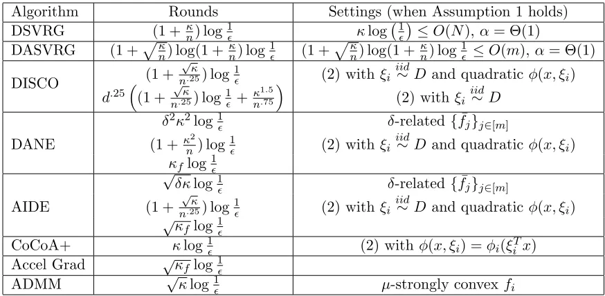
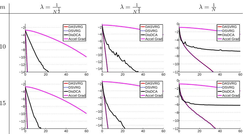
Recently, there have been many distributed optimization algorithms proposed for prob-lem (1) when f is strongly convex. We list several of them, including a distributed imple-mentation of the accelerated gradient method (Accel Grad) by Nesterov (2013), in Table 1 and present their rounds and key assumptions for a clear comparison. Except DSVRG and DASVRG, all algorithms in Table 1 belong to F0 (i.e.,Rj =∅).
The O(√κflog(1)) rounds of communication (κf := Lf
µ) of Accel Grad in Table 1 is
directly from the iteration complexity of the single-machine accelerated gradient method, and the O(√κlog(1)) round complexity of centralized ADMM was given by Deng and Yin (2016). The distributed dual coordinate ascent method, including DisDCA (Yang, 2013), CoCoA (Jaggi et al., 2014) and CoCoA+ (Ma et al., 2015), is a class of distributed coordinate optimization algorithms which can be applied to the conjugate dual formulation of (2) when fi(x) = φ(x, ξi) = φi(ξTi x) for φi on R1. By Ma et al. (2015) and Jaggi et al. (2014), CoCoA+ requiresO(κlog(1/)) rounds of communication to find an-optimal solution.2 Therefore, when applicable, both DSVRG and DASVRG with α= Θ(1) require fewer rounds of communication than the methods mentioned above.
Assuming the problem (1) has the form of (2) withξi’s i.i.d. sampled from a distribution
D(denoted byξiiid∼ D), the DANE (Shamir et al., 2014) and DISCO (Zhang and Lin, 2015)
algorithms requireO((1 +
√ κ
n.25) log(1/)) andO((1 +κ 2
n) log(1/)) rounds of communication,
respectively. Hence, DSVRG uses fewer rounds of communication than DANE and fewer than DISCO when κ≤n1.5. If applicable, DASVRG always uses fewer rounds of commu-nication than DISCO and DANE. Furthermore, DANE only has the theoretical guarantee
Algorithm Rounds Settings (when Assumption 1 holds)
DSVRG (1 +nκ) log1 κlog 1≤O(N), α= Θ(1)
DASVRG (1 +pκn) log(1 + κn) log1 (1 +pnκ) log(1 +κn) log1 ≤O(m),α = Θ(1)
DISCO (1 +
√ κ
n.25) log1 (2) with ξi iid
∼D and quadraticφ(x, ξi)
d.25
(1 +
√ κ n.25) log
1 +
κ1.5
n.75
(2) with ξiiid∼D
δ2κ2log1 δ-related{f¯j}j∈[m]
DANE (1 + κn2) log1 (2) with ξiiid∼D and quadraticφ(x, ξi)
κflog1
√
δκlog1 δ-related{f¯j}j∈[m]
AIDE (1 +
√ κ
n.25) log1 (2) with ξi iid
∼D and quadraticφ(x, ξi)
√
κflog1
CoCoA+ κlog1 (2) with φ(x, ξi) =φi(ξiTx)
Accel Grad √κflog1
ADMM √κlog1 µ-strongly convex fi
Table 1: Rounds and settings of different distributed optimization algorithms. Except DSVRG and DASVRG, all algorithms in this table only require α= 0 (i.e., they do not require a subset Rj sampled with replacement).
mentioned above when it is applied to quadratic problems. Also, DISCO only applies to self-concordant functions with easily computed Hessian3 and makes strong statistical as-sumptions on the data points. On the contrary, DSVRG and DASVRG works for a more general problem (1) and do not assume ξi
iid
∼D for (2).
In each iteration, DANE requires solving a non-trivial sub-problem to optimality. Reddi et al. (2016) proposed an INEXACTDANEalgorithm that is similar to DANE but only needs to solve the sub-problem approximately and still achieves the same round complexity as DANE up to a logarithmic factor. Applying the acceleration techniques developed by Frostig et al. (2015) and Lin et al. (2015) to INEXACTDANE, Reddi et al. (2016) further proposed an Accelerated Inexact DanE (AIDE) algorithm that matches the round complexity of DISCO up to a logarithmic factor.
Shamir (2016) consider a without-replacement SVRG which, if implemented in a dis-tributed way, is similar to the DSVRG proposed here. The main difference between his method and DSVRG is that his method sequentially accesses the data points in Sj while
while DSVRG accesses the data points in Rj for the local update. Since Shamir (2016)
assumes that the concatenation of {Sj}j∈[m] forms a random permutation of {fi}[N], his method essentially performs the iterative update of SVRG by sampling from{fi}[N]without replacement. When κ is smaller than N and is not extremely small (the same as what DSVRG requires), his method obtains the same round complexity as DSVRG. However, his complexity analysis only applies for quadratic {fi}[N]. Koneˇcn´y et al. (2016) proposed a
3. The examples in Zhang and Lin (2015) all take the form offi(x) =φi(ξiTx) for some functionφionR1,
Federated SVRG algorithm which is also a distributed implementation of SVRG and can be viewed as a special case of INEXACTDANEwith specific choices of parameters (Reddi et al., 2016). However, the performance analysis of INEXACTDANEunder those specific choices of parameters is only available when{fi}[N] are quadratic and δ-related.
The methods in comparison in Table 1 are centralized methods which are typically implemented in a star network with a center server. There also exist many distributed (sub)gradient methods (Nedi´c and Ozdaglar, 2007, 2009; Duchi et al., 2012; Jakoveti´c et al., 2012; Chen and Ozdaglar, 2012; Jakoveti´c et al., 2014; Beck et al., 2014; Shi et al., 2015a,b; Aybat et al., 2015) and distributed ADMM methods (Boyd et al., 2011; Wei and Ozdaglar, 2012; Mota et al., 2013; Shi et al., 2014; Chang et al., 2015; Makhdoumi and Ozdaglar, 2017; Deng and Yin, 2016; Mokhtari et al., 2016) for decentralized optimization over general networks. In general, the decentralized distributed methods require more rounds of com-munication than the centralized ones. For example, the number of comcom-munication rounds needed by the decentralized ADMM in Makhdoumi and Ozdaglar (2017) is O(√κlog(1)) multiplied by a network-dependent factor that is typically greater than one.
3. Lower Bounds on Rounds of Communication
In this section, we first define a broad family of distributed (extended) first-order methods which contains many existing distributed optimization algorithms in the literature. Then, we prove the lower bounds for the round complexity for this family of algorithms to find an -optimal solution for (1) under Assumption 1 withµ >0 and µ= 0, respectively.
The algorithms in the family we consider consist of a data distribution stage where the functions {fi}i∈[N] are distributed ontom machines, and a distributed computation stage
where, in each round, machines can not only use first-order information of the functions stored locally but also apply preconditioning using local second-order information.
Definition 1 (Distributed (extended) first-order algorithms Fα) Suppose there is a
stage of data distribution where {fi}i∈[N] are distributed to m machines such that:
1. The index set [N]is randomly and evenly partitioned intoS1, S2, . . . , Sm with|Sj|=n
for j= 1, . . . , m.
2. A multi-set Rj of size αn is created by sampling with replacement from [N] for j =
1, . . . , m, where α≥0 is a constant. When α= 0, we have Rj =∅ for all j.
3. Let Sj0 =Sj∪Rj. Machine j acquires functions in {fi}i∈S0j for j= 1, . . . , m.
We say an algorithm A for solving (1) belongs to the family Fα (A ∈ Fα) of distributed (extended) first-order algorithms if the machines do the following operations in rounds:
1. Machinejmaintains a local working set of vectorsWj ⊂Rdinitialized to beWj ={0},
2. In each round, for arbitrarily many times, machine j can add anyw∈Rd to W j if w
satisfies (c.f. Arjevani and Shamir (2015))
γw+ν∇Fj(w)∈span
w0,∇Fj(w0),(∇2Fj(w0) +D)w00,(∇2Fj(w0) +D)−1w00
w0, w00∈Wj, D is diagonal,∇2Fj(w0) and(∇2Fj(w0) +D)−1 exist
(5)
for some constants γ ≥ 0 and ν ≥ 0 with γν = 06 , where Fj = Pi∈Uj⊂S0
jfi with an
arbitrary subset Uj of Sj0.
3. At the end of the round, all machines can simultaneously send any vectors in Wj
to any other machines, and each machine can add the vectors received from other machines to its local working set.
4. The final output is a vector in the linear span of Wj for any j.
We use A({fi}i∈[N],{Sj0}j∈[m], H) to represent the output vector of A when it is applied
to (1) for H rounds with the inputs {fi}i∈[N] and the sets {Sj0}j∈[m] generated in the data
distribution stage described above.
Besides the randomness due to the data distribution stage, the algorithm A itself can be a randomized algorithm. Hence, the outputA({fi}i∈[N],{Sj0}j∈[m], H) can be a random
vector. Next, we provide some discussions on this class of algorithms.
In Fα, machines can only share iterates but not data points explicitly. Therefore, the
sets {Sj0}j∈[m] will not be changed during the algorithm. The class Fα allows gradient
updatew=w0−η∇Fj(w0) withη >0 in local computation, which corresponds to (5) with γ = 1, ν = 0. It also allows proximal mapping update w = arg minv 21ηkv−w0k2 +F
j(v)
withη >0 in local computation, which has an optimality conditionw+η∇Fj(w) =w0 and
thus corresponds to (5) withγ = 1, ν =η. As a result, the classF0 covers distributed Accel
Grad, ADMM, DANE and AIDE. Although the algorithms inFα can use the local second-order information like ∇2f
i(x) in each machine, Newton’s method is still not contained in
Fα since Newton’s method requires the access to the global second-order information such
as ∇2f(x) (machines are not allowed to share Hessian matrices with each other). That
being said, one can still use a distributed iteration method which can multiply∇2f
i(x) to a
local vector in order to solve the inversion of∇2f(x) approximately. This scheme will lead
to a distributed inexact Newton method such as DISCO, which also belongs to F0. The DSVRG and DASVRG algorithms proposed in this paper belong toFα withα >0.
We are ready to present the lower bounds for the rounds of communications.
Theorem 2 Suppose m ≥(e+ 4 max{1, α})2 and there exists an algorithm A ∈ Fα with
the following property:
“For any > 0 and any N convex functions {fi}i∈[N] satisfying Assumption 1 with
µ > 0 and κ ≥ 1.5n, there exists H such that the output xˆ =A({fi}i∈[N],{Sj0}j∈[m], H)
satisfiesE[f(ˆx)−f(x∗)]≤, where the sets{Sj0}j∈[m] are generated as in Definition 1.” Then, with k≡ d(e+ 4 max{1, α}) logme, we must have
H≥ p
2κ/(3n) +k−1−√k
4k√k
! log
1−1
e
µ
kx∗k2 4
≥Ω˜ s
κ/n+α (α+ 1)3log
µ
kx∗k2
!
In the definition of Fα, we allow the algorithm to access both randomly partitioned data and independently sampled data, and allow the algorithm to use local Hessian for preconditioning. This makes our lower bounds in Theorem 2 stronger: Even with more options in distributing data and with algorithms more powerful than first-order methods (in terms of the class of operations it can take), the number of rounds needed to find an -optimal solution still cannot be reduced.
The κ ≥ 1.5n condition is not critical because, when κ ≤ n132−2δ <1.5n for a constant 0< δ < 12, we will show in Proposition 15 in Section 5.2 that DSVRG only needsO(log(1δlog/n)) rounds, which almost meets the trivial lower bound Ω(1).
A similar result can be obtained for the non-strongly convex case.
Theorem 3 Suppose m ≥(e+ 4 max{1, α})2 and there exists an algorithm A ∈ Fα with
the following property:
“For any > 0 and any N convex functions {fi}i∈[N] satisfying Assumption 1 with µ= 0, there existsH such that the outputxˆ=A({fi}i∈[N],{Sj0}j∈[m], H)satisfiesE[f(ˆx)− f(x∗)]≤, where the sets{Sj0}j∈[m] are generated as in Definition 1.”
Then, with k≡ d(e+ 4 max{1, α}) logme, we must have H≥
q 1−1
e
Lkx∗k2
64k3n.
4. Proofs of Main Results
In this section, we will provide the proofs for Theorem 2 and 3. Before presenting all technical details, we will first give an informal sketch of the proofs.
4.1 Sketch of Proof for Main Results
We will only provide an informal proof sketch for Theorem 2. The proof of Theorem 3 follows a similar strategy.
Let k be an integer with k = Θ(log(m)), µ0 = nµ and κ0 = µL0. For simplicity, we
assume mk is an integer in this proof sketch although Theorem 2 and 3 hold without this assumption. LetE0 ={0} where0 is the all-zero vector inRb and let Et be the subspace
ofRb consisting of the vectors whose non-zero values only appear in the firsttcoordinates. Motivated by the proof for the lower bound of the iteration complexity of first-order methods (Nesterov, 2013), we construct a convex quadratic function ¯p : Rb → R and represent it as the average ofk convex quadratic functionsps:Rb →R fors= 1,2, . . . , k. In particular, we construct ¯p(w) = 12wTΣw+qTw+ µ20kwk2 = 1
k
Pk
s=1ps, where ¯ps(w) = 1
2w TΣ
sw+qsTw+µ 0 2kwk
2 for s= 1,2, . . . , k. We are able to choose Σ, Σ
s, q and qs here
such that the following properties are satisfied
1. The matrix Σ = 1kPk
s=1Σs. The matrix Σ is tridiagonal and the matrix Σs is block
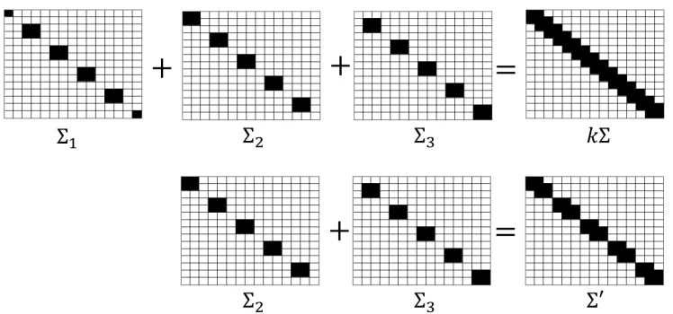
diagonal with a 2×2 block andk−2 consecutive zero entries alternatively appearing along its diagonal. The sparsity patterns of Σ and Σs can be seen in Figure 1 in an
example withb= 15 and k= 3.
2. The vector q= 1kPk
s=1qs withq, qs∈E1 fors= 1, . . . , k.
Figure 1: The sparsity pattern of Σ and Σ0 when U ={2,3},b= 15 andk= 3.
4. The vectorw∗ = arg minwp¯(w) is non-zero in all coordinates and, whenbis sufficiently larger than t,kwˆ−w∗k2 ≥Ω((1−√1
κ0)
2t) for any ˆw∈E t.
Because the gradient ∇p¯(w) = (Σ +µ0I)w+q, where Σ is tridiagonal and q ∈ E1,
if a first-order method is applied to minwp¯(w) with an initial solution of 0, the solution
will stay in Et after t iterations. According to the 4th property above, a large number of
iterations is needed for the first-order method to achieve an -optimal solution. We will use a similar argument to show that, when minwp¯(w) is solved by a distributed first-order
method but each machine does not have a full collection of {ps}s∈[k], a large number of
rounds of communication is needed in order to find an -optimal solution.
Suppose a machine can only locally access the functions in {ps}s∈U with U $ [k]. By the sparsity patterns of Σ and Σs, Σ0 = Ps∈UΣs will be block diagonal with the size of
each block being at most (k+ 1)×(k+ 1). The sparsity patterns of Σ0 can be seen in Figure 1 for an example with U = {2,3}, b = 15 and k = 3. Since q, qs ∈ E1, if the
local computation of this machine starts with an initial solution in Et and the solution is
updated only using linear combinations of gradients∇ps(w) = (Σs+µ0I)w+qs fors∈U,
this machine can only produce a solution inEt+k no matter how many local iterations are
performed. According to the 4th property above, this machine has to receive a solution outsideEt+k from other machines in order to make progress in approximtingw∗. Hence, if
no machine in a distributed first-order method has a full collection of{ps}s∈[k], many rounds
of communication is needed in order to generate an -optimal solution for minwp¯(w).
Since ¯p is the average of onlyk= Θ(log(m)) functions while the communication lower bound is given for minimizing the average of N functions, we will make a few copies of {ps}s∈[k] and add some zero functions to them. In particular, let v = mk and {gi}i∈[N]
be the multi-set of functions on Rb that consists of v copies of {ps}s∈[k] and N −vk zero
functions. Therefore, ¯g(w)≡ N1 PN
i=1gi(w) = p¯(nw) so thatw∗ = arg minw¯g(w). In addition,
each gi is L-smooth due to the 3rd property above and g is µ 0
n-strongly (i.e., µ-strongly)
convex becausem gi’s are µ0-strongly convex andN −m gi’s are zero.
Suppose an algorithm in Fα is applied to minwg¯(w) with the initial solution 0. Each
func-tions from {gi}i∈[N] by random sampling with replacement. Since k = Θ(log(m)) and {gi}i∈[N] contains only vk = m functions from {ps}s∈[k] and N −m zero functions, we
can show that, with a high probability, no machine will receive k or more functions from {ps}s∈[k]. According to the previous discussion, the number of non-zero coordinate in the solution generated by the algorithm will only increase by at most k between two consec-utive rounds of communication. In other words, if ˆw is the solution found by Fα after H rounds of communication, we must have ˆw ∈ Et with t = Hk. By the 4th property
above, the distance kwˆ−w∗k2 ≥Ω((1− √1 κ0)
2t). Since ¯g is strongly convex, this distance
implies an objective function gap of ¯g( ˆw)−¯g(w∗) ≥ Ω((1− √1 κ0)
2t). Hence, in order to
ensure ¯g( ˆw)−g¯(w∗)≤, with a high probably, the rounds of communication must satisfy H = kt ≥Ω(√κ0) log 1
= Ω(pκ
n) log 1
. This provides the lower bounds for the rounds of communication we found in this paper. Finally, we show that the same lower bound can be proved without having any zero function in the N functions. To do so, we raise the di-mension of the problem frombtod=nbby constructing a problem like (1), where{fi}i∈[N] consists of vncopies of {ps}s∈[k]with the first v copies defined on the first bcoordinates of x, the secondv copies defined on the secondbcoordinates ofxand so on. Problem (1) with such{fi}i∈[N]can be solved asnindependent problems onRbwith each problem equivalent to minwg¯(w) so that the same communication lower bound can be obtained.
4.2 Some Definitions and Lemmas
Before we start the formal proof for Theorem 2, some definitions and technical lemmas are provided in this section. Given a vector x∈Rd and a set of indicesD⊂[d], we use xD to
represent the sub-vector of xthat consists of the coordinates of xindexed by D.
Definition 4 A functionf :Rd→Risdecomposablewith respect to a partitionD1, . . . , Dr
of coordinates [d] if f(x) = g1(xD1) +· · ·+g
r(x
Dr) with g l :
R|Di| → R for l = 1, . . . , r.
A set of functions {fi}i∈[N] issimultaneously decomposable with respect to a partition
D1, . . . , Dr if each fi is decomposable with respect toD1, . . . , Dr.
It follows the Definition 1 and Definition 4 straightforwardly that:
Proposition 5 Suppose the functions{fi}i∈[N]in (1) are simultaneously decomposable with
respect to a partition D1, . . . , Dr so that fi(x) = Prl=1gli(xDl) with g l
i : R|Dl| → R for
i= 1, . . . , N and l= 1, . . . , r. Let x∗ be the optimal solution of (1). We must have
x∗D
l∈arg min w∈R|Dl|
¯
gl(w)≡ 1 N
N
X
i=1 gil(w)
, for l= 1,2, . . . , r. (6)
Moreover, any algorithm A ∈ Fα, when applied to{fi}i∈[N], becomes decomposable with respect to the same partitionD1, . . . , Dr in the following sense: Forl= 1, . . . , r, there exists
an algorithm Al∈ Fα such that, after any number of rounds H,
E[f(ˆx)−f(x∗)] =
r
X
l=1
E[¯gl( ˆwl)−¯gl(x∗Dl)],
Proof The proof of this proposition is straightforward. Since {fi}i∈[N] in (1) are simulta-neously decomposable with respect to a partitionD1, . . . , Dr, we have
f(x) = 1 N
N
X
i=1 r
X
l=1
gli(xDl) = r
X
l=1
¯ gl(xDl)
so that the problem (1) can be solved by solving (6) for eachl separately andx∗D
l must be
the solution of the l-th problem in (6).
In addition, the functionFj in Definition 1 is also decomposable with respect to the same
partitionD1, . . . , Dr. As a result, its gradient∇Fj(x) also has a decomposed structure in the
sense that the block [∇Fj(x)]Dlonly depends onxDl. Similarly, its Hessian matrix∇ 2F
j(x)
is a block diagonal matrix with r blocks and the l-th block only depends on xDl. These
properties ensure that each operationAis able to apply (as in Definition 1) to somex∈Rd can be decomposed intor independent operations applied on xD1, xD2, . . . , xDr separately.
Hence, given the sets {S0
j}j∈[m], the sequence of operations conducted byA on xDl can be
viewed as an algorithmAl∈ Fαapplied to{gil}i∈[N]so that ˆwl=Al({gil}i∈[N],{Sj0}j∈[m], H)
is indeed the sub-vector ˆxDl of the vector ˆx =A({fi}i∈[N],{S 0
j}j∈[m], H) for l= 1,2, . . . , r
and any H.
Because m≥(e+ 4 max{1, α})2 and k≡ d(e+ 4 max{1, α}) logme, we can show that m
k ≥
m
1.25(e+ 4 max{1, α}) logm ≥
e+ 4 max{1, α} 2.5 log(e+ 4 max{1, α}) ≥
e+ 4
2.5 log(e+ 4) >3
for any α ≥0, where we use the fact that 1.25x ≥ dxe forx ≥4 and the fact that logxx is monotonically increasing on [e,+∞). In the rest of the paper, we define
v≡jm k k
and θ≡ vk m.
It is easy to show that 23 <1−mk < θ≤1, where the first inequality is because mk >3 and the second and the last inequalities are by the definitions ofv and θ.
4.3 Proof for Theorem 2
Now we are ready to give the proof for Theorem 2 in this subsection. Let
µ0≡ µn θ , κ
0 ≡ L µ0 =
θκ n >
2κ
3n ≥1. (7)
We first generalize the machinery by Arjevani and Shamir (2015) to construct k functions onRb whereb=uk for some integersk, u≥1. The values ofkandu will be specified later. In particular, fori, j= 1, . . . , b, letδi,j be anb×bmatrix with its (i, j) entry being one and
others being zeros. LetM0, M1, . . . , Mb−1 be b×bmatrices defined as
Mi =
δ1,1 fori= 0
δi,i−δi,i+1−δi+1,i+δi+1,i+1 for 1≤i≤b−2 δb−1,b−1−δb−1,b−δb,b−1+
√
κ0+k−1+3√k √
κ0+k−1+√kδb,b fori=b−1.
Fors∈[k], let
Σs = u−1 X
i=0
Mik+s−1. (9)
For example, when u= 2 andk= 3 (sob= 6), the matrices Σs’s are given as follows
Σ1=
1 0 0 0 0 0
0 0 0 0 0 0
0 0 1 −1 0 0
0 0 −1 1 0 0
0 0 0 0 0 0
0 0 0 0 0 0
,Σ2=
1 −1 0 0 0 0
−1 1 0 0 0 0
0 0 0 0 0 0
0 0 0 1 −1 0
0 0 0 −1 1 0
0 0 0 0 0 0
,
Σ3=
0 0 0 0 0 0
0 1 −1 0 0 0
0 −1 1 0 0 0
0 0 0 0 0 0
0 0 0 0 1 −1
0 0 0 0 −1 K
,
whereK =
√
κ0+k−1+3√k √
κ0+k−1+√k.
We define kfunctions p1, . . . , pk:Rb →Ras follows
ps(w) =
L 4 h
1−µL0wTΣ1w
2 −
1− µL0e>1wi+µ20kwk2 fors= 1 L
4 h
1−µL0wTΣs2 wi+µ20kwk2 fors= 2, . . . , k, (10)
wheree1 = (1,0, . . . ,0)T ∈Rb, and denote their average by
¯ p≡ 1
k
k
X
s=1 ps=
L−µ0 4k " 1 2w T k X s=1 Σs !
w−eT1w #
+µ
0
2kwk
2. (11)
According to (7), we have 1− µL0 > 0 so that ps for any s ∈ [k] and ¯p are all µ0-strongly
convex functions. It is also easy to show that, for each s,λmax(Σs)≤4 so that ∇ps has a
Lipschitz continuity constant of L1−µL0+µ0 =L and ps is L-smooth.
Next, we characterize the optimal solution of minw∈Rbp¯(w).
Lemma 6 Let h∈Rbe the smaller root of the equationh2−2κ0−1+2κ0−1k
h+1 = 0,namely,
h≡ √
κ0+k−1−√k √
κ0+k−1+√k. Then,w
∗ = (w∗
1, w∗2, . . . , w∗b)T ∈Rb with
wj∗=hj, for j= 1,2, . . . , b (12)
Proof By (9), we have
k X
s=1 Σs=
2 −1 0 0 0 0
−1 2 −1 0 0 0
0 −1 2 −1 0 0
..
. ... . .. . .. . .. ...
0 0 0 −1 2 −1
0 0 0 0 −1
√
κ0+k−1+3√k
√
κ0+k−1+√k
.
With this tridiagonal structure in its Hessian matrix, ¯p(w) is related to but different from the functions constructed by Nesterov (2013) and Lan and Zhou (2017) to establish the iteration lower bound for single-machine first-order algorithms. We can show that the optimal solution of minw∈Rbp¯(w) must satisfy the following optimality conditions
w∗2−2
κ0−1 + 2k κ0−1
w∗1+ 1 = 0 wj∗+1−2
κ0−1 + 2k κ0−1
wj∗+wj∗−1 = 0, forj= 2,3, . . . , b−1 (13)
− √
κ0+k−1 + 3√k √
κ0+k−1 +√k +
4k κ0−1
!
w∗b +w∗b−1 = 0.
We can easily verify that w∗j =hj forj = 1,2, . . . , b satisfy all equations in (13) such that
w∗ is the optimal solution of minw∈Rbp¯(w).
We claim that{ps}s∈[k]in (10) has the following property according to our construction. Lemma 7 Suppose U is a strict subset of {ps}s∈[k] defined in (10), andq is an arbitrary linear combination of some functionsps in U. The Hessian of q is a block diagonal matrix
where each block is a square matrix of a size at most k.
Proof There must exist some s0 ∈ [k] with ps0 ∈/ U. Since q is a linear combination of ps’s in U, according to the construction in (10), the Hessian of q is a tridiagonal matrix
because it is a linear combination of a diagonal matrix (the Hessian of µ20kwk2) and all the
matrices Σs defined in (9) except Σs0. We note that Σs0 is the only matrix among all Σs’s
that has non-zero entries in the positions (s0−1 +ik, s0+ik) and (s0+ik, s0−1 +ik) for i= 0,1, . . . , u−1 and both the row and column indices of these positions are equally spaced with a gap ofk. Therefore, without Σs0 involved in the linear combination, the tridiagonal
Hessian ofq becomes block diagonal with each block of a size at mostk.
Lemma 8 For any b=uk with integers k, u≥1, let{gi}i∈[N] be the multi-set of functions onRb that consists of vcopies of {ps}s∈[k]defined as (10) and N−vk zero functions. More
specifically,
gi(w) =
ps(w) if i=s, s+k, s+ 2k, . . . , s+ (v−1)k,
0 if i≥vk+ 1. (14)
Suppose an algorithm A ∈ Fα is applied to{gi}i∈[N] to solve
min
w∈Rb¯g(w)≡
1 N
N
X
i=1
gi (15)
and the sets {Sj0}j∈[m] are generated as in Definition 1. Let E be the random event that
none of the m machines has all functions in {ps}s∈[k]. Let wˆ =A({gi}i∈[N],{Sj0}j∈[m], H).
Then, for any >0 and k≥1, there exist u and b=uk such that E[g( ˆw)−g(w∗)|E]≤
only ifH ≥ √
κ0+k−1−√k 4k√k
logµkw4∗k2.
Proof Let w∗ ∈ Rb defined as (12). Since ¯g = 1 N
PN
i=1gi = Nv
Pk
s=1ps = θnp¯, we have
w∗ = arg minw∈Rbp¯(w) = arg minw∈
Rbg¯(w) by Lemma 6.
Let E0 ={0}, where 0 is the all-zero vector inRb and let Et be the linear space in Rb spanned by the unit vectors e1, . . . , et for t = 1, . . . , b, where es ∈ Rb has one in its s-th component and zeros in other components.
Because A is applied to (15), by Definition 1, the working setWj in machinej in each
round can be updated for arbitrarily many times by including a vectorw such that
γw+ν∇Fj(w)∈span
w0,∇Fj(w0),(∇2Fj(w0) +D)w00,(∇2Fj(w0) +D)−1w00
w0, w00 ∈Wj, D is diagonal,∇2Fj(w0) and (∇2Fj(w0) +D)−1 exist
(16)
for some constantsγ≥0 andν ≥0 withγν 6= 0, whereFj =Pi∈Uj⊂Sj0gi with an arbitrary
subset Uj of Sj0. Suppose event E happens such that Sj0 does not contain all functions in
{ps}s∈[k] for anyj. The set Uj in (16) will be a strict subset of{ps}s∈[k] so that, according
to Lemma 7, the Hessian matrix ∇2F
j in (16) is block-diagonal with a block size at most
k. BecauseFj is always a quadratic function, such a property of its Hessian matrix means,
as long as Wj is contained byEt, any vector w satisfying (16) will be in Et+k. Therefore,
we can show that, at the beginning of round ` in algorithmA, if ∪jWj ⊂Et, then at the
end of round ` (and at the beginning of round `+ 1), we have ∪jWj ⊂ Et+k. Using this
finding and the fact that ∪jWj ={0}=E0 initially, we conclude that, afterH rounds in A, we must have∪jWj ⊂EHk. Lett=Hk. Since ˆw=A({gi}i∈[N],{Sj0}j∈[m], H), we must
have ˆw∈Et ifE happens.
By (12), we can show that
kw∗k2 =
b
X
j=1
(w∗j)2=
b
X
j=1
h2j = h
2(1−h2b)
Because ¯pdefined in (11) is µ0-strong convex, we have
2
µ0E[¯p( ˆw)−p¯(w ∗)|E]≥
E[kwˆ−w∗k2|E]≥ b X
j=t+1 E[(w∗j)
2|E]≥ h2t+2(1−h2b−2t)
1−h2 ≥
kw∗k2(h2t−h2b) 1−h2b
where the second inequality is because ˆw ∈ Et and the third inequality is due to (17).
For any k ≥ 1, when u is large enough so b = uk is large enough, the inequality above implies E[¯p( ˆw)−p¯(w∗)|E]≥ µ
0kw∗k2h2t
4 =
µ0kw∗k2
4 √
κ0+k−1−√k √
κ0+k−1+√k 2t
. Based on this inequal-ity, when E[¯g( ˆw) −g¯(w∗)|E] ≤ , or equivalently, when E[¯p( ˆw) − p¯(w∗)|E] ≤ nθ, we must have logµ0θ4knw∗k2≤2tlog1 + 2
√ k √
κ0+k−1−√k
≤ √ 4t√k
κ0+k−1−√k,which further implies H= kt ≥
√
κ0+k−1−√k 4k√k
log
µkw∗k2
4
.
In Lemma 8, the requirement of a large enoughb=ukis necessary since, ifbis fixed and the number of rounds H satisfies Hk ≥b, the solution ˆw =A({gi}i∈[N],{Sj0}j∈[m], H) can
be non-zero in all dimensions so that it may equalw∗. If this happens,g( ˆw)−g(w∗)≤for anyso that the lower bound forHin Lemma 8 does not hold. Because the communication lower bound we study does not depend on the dimension of the problem, we construct the functions with a dimension higher than Hk so that there are dimensions that will not be reached by the generated solutions so that the optimality gap has to reduce to zero slowly. We now complete the proof of Theorem 2 by constructingN special functions {fi}i∈[N] on Rd withd=nband b =uk for a sufficiently large u based on {ps}s∈[k] defined as (10),
so that any algorithm A ∈ Fα, when applied to {fi}i∈[N], will need at least the targeted
amount of rounds of communication.
For a large enough u, we partition the set of indices [d] = {1, . . . , d} into n disjoint subsets D1, D2, . . . , Dn with|Dl|=b and Dl={b(l−1) + 1, , b(l−1) + 2, . . . , bl}. For any
l∈[n] ands∈[k], letql,s(x) be a function onRd defined as
ql,s(x)≡ps(xDl), (18)
where{ps}s∈[k]is defined as (10). By its definition, the functionql,s(x) only depends on the
bcoordinates ofxindexed byDl. Therefore, we obtainnkdifferent functions{ql,s}l∈[n],s∈[k].
Finally, we define{fi}i∈[N]to be a set that consists ofvcopies of{ql,s}l∈[n],s∈[k]andN−vkn zero functions. In other words, the non-zero functions in the set {fi}i∈[N] we constructed in this way constitutes a multi-set as follows
p1(xD1), p2(xD1), · · ·, pk(xD1), · · · , p1(xD1), p2(xD1), · · ·, pk(xD1)
p1(xD2), p2(xD2), · · ·, pk(xD2), · · · , p1(xD2), p2(xD2), · · ·, pk(xD2)
..
. ... ... ... ... ... ... ... ...
p1(xDn), p2(xDn), · · ·, pk(xDn), . . . , p1(xDn), p2(xDn), · · ·, pk(xDn) , (19)
where thel-th row consists ofv copies of {ps}s∈[k] applied onxDl.
Because of Lemma 6 and the fact that
f(x) = 1 N
N
X
i=1
fi(x) =
v N n X l=1 k X s=1
ql,s(x) =
v N n X l=1 k X s=1
ps(xDl) = θ n n X l=1 ¯
the optimal solution x∗ for (1) with {fi}i∈[N] constructed as (19) is x∗ = 1n ⊗w∗ =
(w∗, w∗, . . . , w∗)T where w∗ ∈
Rd is defined as (12) and repeated forntimes in x∗.
Now, we want to verify that the functions {fi}i∈[N]satisfy our assumptions. In fact, we have shown thatps isL-smooth for eachs∈[k]. Sincefi is either a zero function or equals
ps(xDl) for some l ∈[n] and s∈[k], the function fi is L-smooth for each i∈ [N] as well.
Since ¯p is µ0-strongly convex (on Rb) and µ0 = nµθ , the function f defined in (1) must be µ-strongly convex (onRd) according to the relationship (20).
According to its construction, {fi}i∈[N] are simultaneously decomposable with respect to the partition D1, . . . , Dn with Dl={b(l−1) + 1, b(l−1) + 2, . . . , bl} (see Definition 4).
In fact,fi(x) =ps(xDl) for some s∈[k] and l∈[n] so thatfi(x) can be represented as
fi(x) = n
X
l=1
gil(xDl), (21)
where gli ∈ {ps}s∈[k] for exactly one l ∈ [n] and gil ≡ 0 for other l’s. Moreover, for any l∈[n], the following equality holds between the two multi-sets
{gli}i∈[N]={gi}i∈[N], (22)
where{gi}i∈[N]are defined as (14).4 By Proposition 5,Acan be decomposed with respective
to the same partitionD1, D2, . . . , Dn intoA1, . . . ,An∈ Fα and Al is applied to
min
w∈Rb
(
¯ gl≡ 1
N
N
X
i=1
gil= 1 N
N
X
i=1 gi= ¯g
)
, (23)
which is exactly the problem (15) and has the form of (1). Recall Definition 1 for the procedure of generating Sj0 = Sj ∪Rj, When {fi|i ∈ Sj0} is allocated to machine j for
algorithm A, what happens at the same time is that {gl
i|i∈Sj0} is allocated to machinej
for algorithm Al forl= 1,2, . . . , n.
We now focus on the solution generated by Al for somel. For machinej inAl, letY1,j
be the number of functions in {ps}s∈[k] (repetitions counted) that are contained inSj and
Y2,j be the number of functions in{ps}s∈[k] (repetitions counted) that are contained inRj.
Due to (14) and (22), exactly vk functions in{gl
i}i∈[N] are from{ps}s∈[k] and the other N−vk functions are zero. Hence,Y1,jhas a hypergeometric distribution where Prob(Y1,j=
r) equals the probability ofr successes inndraws, without replacement, from a population of size N that contains vk successes. Let r = elogm. According to Chvatal (1979) and
4. The equation (22) does not meansgil=gifor anylandi. It only means, for anylandi, there exists an
vk N ≤
1
n, we have Prob(Y1,j ≥r)≤ vkn
N r
rn−vkn/N
n−r
n−r ≤ 1
r
rn−1 n−r
n−r
,which implies
Prob(Y1,j ≥elogm) ≤
1 elogm
elogm
n−1 n−elogm
n−elogm
=
1 elogm
elogm
1 + elogm−1 n−elogm
n−elogm
<
1 elogm
elogm
eelogm−1 = 1 e
1 logm
elogm
≤ 1 e
1 2 log(e+ 1)
elogm ≤ 1
em2, (24)
where the second inequality is because (1 + x1)x < e, the third inequality is because m ≥ (e+ 4 max{1, α})2 ≥(e+ 1)2, and the last inequality is because (2 log(e+ 1))e> e2.
On the other hand, we have Y2,j = 0 when α = 0 and Y2,j =Pi∈Rj1gli∈{ps}s∈[k] when
α > 0, where 1gl
i∈{ps}s∈[k] for i ∈ Rj are αn i.i.d. binary random variables which equal
one with a probability of vkN and zero with a probability of 1− vkN. Suppose α > 0. The mean and the variance of1gl
i∈{ps}s∈[k] are
θ n and
θ n(1−
θ
n), respectively. Hence, by Bernstein
inequality (Uspensky, 1937), we have
Prob(Y2,j ≥4 max{1, α}logm) ≤ Prob(Y2,j> αθ+ 3 max{1, α}logm)
≤ exp −
1
2(3 max{1, α}logm)2 αθ 1−nθ
+ max{1, α}logm !
≤ exp −
1
2(3 max{1, α}logm)2
2 max{1, α}logm !
≤ exp (−2 max{1, α}logm)≤ 1
m2, (25)
where the first inequality is because max{1, α}logm > αθ and the third inequality is because max{1, α}logm≥αθ 1−nθ
. Supposeα= 0. (25) holds trivially.
Combining (24) and (25) for j= 1,2, . . . , mand using the union bound, we have
Prob(Y1,j+Y2,j <(e+ 4 max{1, α}) logm forj= 1,2, . . . , m)≥1−
2 m.
Therefore, we have shown that, with a probability of at least 1−2
m, the multi-set{g l
i|i∈Sj0}
contains fewer than (e+4 max{1, α}) logm≤kfunctions from{ps}s∈[k](repetition counted)
for any j∈[m]. In other words, with a probability of at least 1−m2, no machine inAl has
all of the functions in{ps}s∈[k]. If the event that “none of the mmachines has all functions
in{ps}s∈[k]” (same as the eventEin Lemma 8) indeed happens inAl, we callAlbad. Then, sincem≥(e+ 4 max{1, α})2, we have actually proved
Prob(Al is bad)≥1− 2
m ≥1− 1
By Proposition 5, afterH rounds, the solutions ˆx=A({fi}i∈[N],{S0
j}j∈[m], H)∈Rdand
ˆ
wl=Al({gli}i∈[N],{Sj0}j∈[m], H)∈R|Dl| forl= 1,2, . . . , nsatisfy
E[f(ˆx)−f(x∗)] =
n
X
l=1
E[¯gl( ˆwl)−g¯l(x∗Dl)] = n
X
l=1
E[¯g( ˆwl)−¯g(x∗Dl)]
≥
n
X
l=1
E[¯g( ˆwl)−g¯(x∗Dl)|Al is bad]Prob(Al is bad)
≥
n
X
l=1
E[¯g( ˆwl)−g¯(x∗Dl)|Al is bad]
1−1 e
.
Therefore, if E[f(ˆx)−f(x∗)]≤, there must exist an l∈[n] such that
E[¯g( ˆwl)−g¯(x∗Dl)|Al is bad]
1−1 e
≤
n. (27)
WhenAlis bad, none of the mmachines inAl has all functions in {ps}s∈[k]. By Lemma 8,
there exist uand b=uk such that (27) happens only if
H ≥
√
κ0+k−1−√k
4k√k
! log
1−1
e
µnkw∗k2
4
=
√
κ0+k−1−√k
4k√k
! log
1−1
e
µkx∗k2
4
,
≥
√κ0−1
4√2k√k
log
1−1
e
µkx∗k2
4
,
which is the desired lower bound after applying κ0 ≥ 2κ 3n. 4.4 Proof for Theorem 3
We provide the proof for Theorem 3 in this subsection by following a similar argument to the proof of Theorem 2. Some notations in the previous sections will be used here but defined differently.
We first use the machinery developed in Section 2.1.1 by Nesterov (2013) to construct kfunctions onRb whereb=uk for some integersk, u≥1. In particular, fori, j = 1, . . . , b, let δi,j be an b×b matrix with its (i, j) entry being one and others being zeros. Let
M0, M1, . . . , Mb−1 be b×bmatrices defined as
Mi=
δ1,1 fori= 0
δi,i−δi,i+1−δi+1,i+δi+1,i+1 for 1≤i≤b−1.
(28)
Here, only the Mb−1 in (28) is different from the Mb−1 in (8). For s ∈ [k], let Σs =
Pu−1
when u= 2 andk= 3 (sob= 6), the matrices Σs’s are given as follows.
Σ1=
1 0 0 0 0 0
0 0 0 0 0 0
0 0 1 −1 0 0
0 0 −1 1 0 0
0 0 0 0 0 0
0 0 0 0 0 0
,Σ2=
1 −1 0 0 0 0
−1 1 0 0 0 0
0 0 0 0 0 0
0 0 0 1 −1 0
0 0 0 −1 1 0
0 0 0 0 0 0
,
Σ3=
0 0 0 0 0 0
0 1 −1 0 0 0
0 −1 1 0 0 0
0 0 0 0 0 0
0 0 0 0 1 −1
0 0 0 0 −1 1
.
We define kfunctions p1, . . . , pk:Rb →Ras follows
ps(w) =
L 4 h
wTΣ
1w
2 −e > 1w
i
fors= 1
L 4 h
wTΣsw 2
i
fors= 2, . . . , k, (29)
wheree1 = (1,0, . . . ,0)T ∈Rb, and denote their average by
¯ p≡ 1
k
k
X
s=1 ps=
L 4k " 1 2w T k X s=1 Σs !
w−eT1w #
. (30)
It is also easy to show that λmax(Σs) ≤4 so that∇ps has a Lipschitz continuity constant
of Lso that ps is L-smooth.
Observing that
k X
s=1 Σs=
2 −1 0 0 0 0
−1 2 −1 0 0 0
0 −1 2 −1 0 0
..
. ... . .. . .. . .. ...
0 0 0 −1 2 −1
0 0 0 0 −1 2
,
we note that the function ¯p(w) defined in (30) is the one studied in Section 2.1.2 by Nesterov (2013) for establishing the lower bound for the iteration complexity for single-machine first-order methods. Following Section 2.1.2 by Nesterov (2013), the optimal solution and the optimal value of minw∈Rbp¯(w) can be characterized as follows.
Lemma 9 (Nesterov (2013)) The vector w∗ = (w∗1, w2∗, . . . , wb∗)T ∈Rb with
w∗j = 1− j
b+ 1, forj= 1,2, . . . , b (31)
is the optimal solution ofminw∈Rbp¯(w). Moreover,kw∗k2≤ b+13 andp¯(w∗) = 8Lk
Lemma 10 (Nesterov (2013)) Let p¯defined as (30). We have
min (w1,...,wt)∈Rt
¯
p(w1, . . . , wt,0, . . . ,0) = L 8k
−1 + 1
t+ 1
.
We can show that{ps}s∈[k] defined in (29) has the following properties.
Lemma 11 Suppose U is a strictsubset of {ps}s∈[k] defined in (10), andq is an arbitrary linear combination of some functionsps in U. The Hessian of q is a block diagonal matrix
where each block is a square matrix of a size at most k.
Proof Same as the proof of Lemma 7.
Lemma 12 For anyb=ukwith integersk, u≥1, let{gi}i∈[N]be the multi-set of functions onRb that consists of vcopies of {ps}s∈[k]defined as (29) and N−vk zero functions. More
specifically, {gi}i∈[N] is defined as (14) but with {ps}s∈[k] defined as (29). Suppose an
algorithmA ∈ Fα is applied to (15) and the sets{Sj0}j∈[m] are generated as in Definition 1.
Let E be the random event that none of the m machines has all functions in {ps}s∈[k]. Let ˆ
w =A({gi}i∈[N],{Sj0}j∈[m], H). Then, for any > 0 and k≥ 1, there exist u and b= uk
such that E[g( ˆw)−g(w∗)|E]≤only if H≥ q
3Lkw∗k2
128k3n.
Proof Let u= 2H+ 1,b= 2Hk+kand w∗ ∈Rb defined as (31). Since ¯g= N1 PNi=1gi= v
N
Pk
s=1ps= θp¯
n, we have w
∗ = arg min
w∈Rbp¯(w) = arg minw∈Rb¯g(w) by Lemma 9.
Let Et defined as in the proof of Lemma 8. Following the same argument as in the
proof of Lemma 8, we can show that, ifE happens, afterH rounds in algorithmA, we must have ∪jWj ⊂EHk, where Wj is the working set of machine j by Definition 1. Let t=Hk.
Since ˆw = A({gi}i∈[N],{S0
j}j∈[m], H), we must have ˆw ∈ Et if E happens. According to
Lemma 10, we have
¯
p( ˆw)≥ min (w1,...,wt)∈Rt
¯
p(w1, . . . , wt,0, . . . ,0) = L 8k
−1 + 1
Hk+ 1
,
which, together with Lemma 9, implies
E
¯
p( ˆw)−p¯(w∗)
kw∗k
E
≥
L 8k
−1 +Hk1+1+ 1− 1 b+1
1 3(b+ 1)
≥ 3L
32k3(H+ 1)2 ≥ 3L 128k3H2.
Based on this inequality, when E[¯g( ˆw) −g¯(w∗)|E] ≤ , or equivalently, when E[¯p( ˆw)− ¯
p(w∗)|E]≤ nθ ≤ 3n2 , we must have H≥ q
Lkw∗k2
64k3n.
The rest of the proof of Theorem 3 is almost identical to that of Theorem 2 so we will only provide a brief sketch. In particular, we will construct N special non-strongly convex functions{fi}i∈[N] onRdwithd=nbfor a sufficiently largebbased on{ps}s∈[k]defined as
(29), and show that any algorithmA ∈ Fα will need at least the targeted amount of rounds
of communication when it is applied to {fi}i∈[N].