On Consistent Vertex Nomination Schemes

On Consistent Vertex Nomination Schemes

Vince Lyzinski [email protected]

Department of Mathematics and Statistics University of Massachusetts Amherst Amherst, MA 01003, USA

Keith Levin [email protected]

Department of Statistics University of Michigan Ann Arbor, MI 48109, USA

Carey E. Priebe [email protected]

Department of Applied Mathematics and Statistics Johns Hopkins University

Baltimore, MD 21218-2608, USA

Editor:Edo Airoldi

Abstract

Given a vertex of interest in a network G1, the vertex nomination problem seeks to find

the corresponding vertex of interest (if it exists) in a second networkG2. A vertex

nom-ination scheme produces a list of the vertices inG2, ranked according to how likely they

are judged to be the corresponding vertex of interest inG2. The vertex nomination

prob-lem and related information retrieval tasks have attracted much attention in the machine learning literature, with numerous applications to social and biological networks. However, the current framework has often been confined to a comparatively small class of network models, and the concept of statistically consistent vertex nomination schemes has been only shallowly explored. In this paper, we extend the vertex nomination problem to a very general statistical model of graphs. Further, drawing inspiration from the long-established classification framework in the pattern recognition literature, we provide definitions for the key notions of Bayes optimality and consistency in our extended vertex nomination framework, including a derivation of the Bayes optimal vertex nomination scheme. In ad-dition, we prove that no universally consistent vertex nomination schemes exist. Illustrative examples are provided throughout.

Keywords: Vertex nomination, graph inference, recommender systems

1. Introduction

Statistical inference on graphs is an important branch of modern statistics and machine learning. In recent years, there have been numerous papers in the literature developing graph analogues of statistical inference tasks such as hypothesis testing (Asta and Shal-izi, 2015; Tang et al., 2017b), classification (Tang et al., 2013; Chen et al., 2016a), and clustering (Luxburg, 2007; Rohe et al., 2011; Sussman et al., 2012; Newman and Clauset, 2016). Moreover, growth in the size and complexity of network data sets have necessitated techniques for network-specific data mining tasks such as link prediction (Liben-Nowell

c

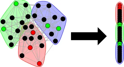
Figure 1: A visual representation of the classical Vertex Nomination framework: Given a community of interest in a network (here the red community) and some examples of vertices that are/are not part of the community of interest (colored red and green, respectively), rank the remaining vertices in the network into a nomination list, with those vertices from the community of interest concentrating at the top of the nomination list.

and Kleinberg, 2007; L¨u and Zhou, 2011); entity resolution and network alignment (Conte et al., 2004; Lyzinski, 2018); and vertex nomination (Coppersmith and Priebe, 2012; Cop-persmith, 2014; Suwan et al., 2015; Fishkind et al., 2015; Lyzinski et al., 2016). Akin to the development of classical statistics, algorithmic advancement has, in many ways, outpaced theoretical developments in these emerging graph-driven domains. This development has been necessitated by the dizzying pace of data generation, but there is nevertheless the need for a firm theoretical context in which to frame algorithmic progress. In this paper, drawing inspiration from the long-established classification framework in the pattern recog-nition literature (Devroye et al., 1997), we provide a rigorous theoretical framework for understanding statistical consistency in the vertex nomination inference task.

The vertex nomination (VN) task, which can be viewed as the graph analogue of the more classical recommender system task (Ricci et al., 2011), has traditionally been stated as follows: given a community of interest in a network and some examples of vertices that are or are not part of a community of interest, vertex nomination seeks to rank the remaining vertices in the network into a nomination list, with those vertices from the community of interest (ideally) concentrating at the top of the nomination list. See Figure 1 for a visual representation of this classical Vertex Nomination framework. In limited-resource settings, vertex nomination tools have proven to be effective in efficiently searching and querying large networks, with applications including detecting fraudsters in the Enron email network (Coppersmith and Priebe, 2012; Marchette et al., 2011; Suwan et al., 2015), uncovering web advertisements that have association with human trafficking (Fishkind et al., 2015), and identifying latent structure in connectome data (Fishkind et al., 2015; Yoder et al., 2018).

not aim to recover the community memberships of any vertices not in the community of interest. Clearly, any method that can recover the community memberships of all vertices in a graph can recover the interesting community, and hence any community detection algorithm can be repurposed for the VN problem just described with minor adaptation (e.g., by ranking vertices according to their probability of membership in the community of interest); see, for example, the spectral vertex nomination scheme of Fishkind et al. (2015). The specific performance of such an adaptation is highly dependent on the fidelity of the base clustering procedure, and the performance is often below that of the semi-supervised VN specific analogues (see Yoder et al., 2018).

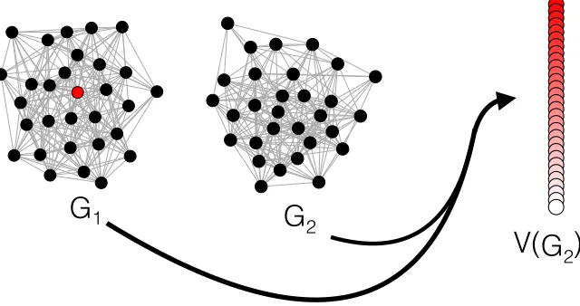
The above formulation of the VN task assumes the presence of strong community struc-ture among the vertices of interest in the graph. In practice, this is often a reasonable assumption, particularly if it is expected that interesting vertices will behave similarly to one another in the network. However, the particular features that mark a vertex as inter-esting are entirely task-dependent. To paraphrase the common proverb, interinter-estingness is in the eye of the practitioner. Interesting vertices may be, for example, those with large network centrality (Jeong et al., 2001; Newman, 2005), those with a particular role in the network (Lusseau and Newman, 2004), or those corresponding to a given user across social networks (Patsolic et al., 2017). In these applications, interesting vertices need not corre-spond precisely to the community structure captured by a generative network model, and hence such cases are ill-described by the community-based VN problem described above. To accommodate this task-dependency and broader notion of interesting vertices, we consider the following generalization and extension of the previously-presented VN problem: Given a vertex of interestv∗ in a graphG1 = (V1, E1), find the corresponding vertex of interestu∗ (if it exists) in a second graphG2= (V2, E2) by ranking the vertices of G2 according to our confidence that they correspond tov∗ in graphG1; see Figure 2 for a visual representation of this VN framework. In this formulation, which is an (potentially) unsupervised infer-ence task, what definesv∗ as interesting is entirely model-dependent, and different network models can highlight different characteristics of interest in the graph. Potential application domains for this VN generalization abound, including identifying users of interest across social network platforms (see, for example, Patsolic et al., 2017), identifying structural sig-nal across connectomes (see, for example, Sussman et al., 2018), and identifying topics of interest across graphical knowledge bases (see, for example, Sun and Priebe, 2013).

G

₂

G

₁

V( )

_G

₂

Figure 2: A visual representation of the generalized Vertex Nomination framework: Given a vertex of interestv∗(colored red) in a graphG1= (V1, E1), find the corresponding vertex of interest u∗ (if it exists) in a second graph G2 = (V2, E2), ranking the vertices ofG2 into a nomination list so that u∗ ideally appears at the top of the nomination list.

of VN consistency—and of VN Bayes optimality—in the two-graph VN framework. This framework is quite general, and further allows us to highlight the similarities and differences between our new VN consistency formulation and its analogue in the classification literature defined in, for example, Devroye et al. (1997).

The paper is laid out as follows. In the remainder of this section, we provide brief overviews of information retrieval as it relates to vertex nomination (Section 1.1) and the Bayes optimal classifier in the classical setting (Section 1.2), and conclude the introduction by establishing notation for the remainder of the paper (Section 1.3). In Section 2, we define the VN problem framework that is the focus of this paper, and in Section 3 we derive the VN analogue of a Bayes optimal scheme. In Section 4, we define a new notion of VN consistency, and we prove that no universally consistent VN scheme exists, providing an interesting contrast to the standard classification setting. We conclude in Section 5 with a short summary comparing and contrasting VN with classical classification and a discussion of implications and future directions.

1.1. Connections to Information Retrieval

Ricci et al. (2011) and Mihalcea and Radev (2011) for the state of the art circa 2010, and concentrate here on recapping more recent graph-based information retrieval techniques.

Many graph-based IR techniques rely on the assumption that similar objects (i.e., doc-uments, webpages, etc.) will lie near one another in a suitably-constructed graph. Indeed, this intuition underlies many graph-based approaches throughout machine learning and re-lated disciplines (see, for example, Belkin and Niyogi, 2003; Zhou et al., 2004). Techniques along these lines have been applied toward many tasks in natural language processing, typi-cally inspired by PageRank (Rothe and Sch¨utze, 2014). Along similar lines, Ma et al. (2012) applied a diffusion-based method (Coifman and Lafon, 2006) to the world wide web graph to yield an approach to ranking for query completion and recommendation. These infor-mation retrieval techniques can be naturally adapted to the vertex nomination problem by treating the vertex or vertices of interest as the object or objects to be retrieved.

The vertex nomination problem also bears similarities to the task of learning to rank (Duh, 2009; Liu, 2009; Li, 2011), in which the goal is to learn an ordering on a set of objects (e.g., documents, images, videos, etc.) according to (estimated) similarity or relevance to a given query object. In the learning to rank literature, graphs usually appear as training instances, with nodes corresponding to objects and edges encoding preferences or similarities among them elicited from users (e.g., an undirected weighted edge may join two documents judged to be similar). The work in Agarwal et al. (2006) is among the earliest to consider the problem of ranking objects in a network. The authors modified the PageRank algorithm to take preference information into account, rather than working solely with the hyperlink graph. In Agarwal (2010), the authors used a data graph encoding object similarities to obtain a regularizer similar to Belkin et al. (2006) on the empirical ranking error, with the target ranking encoded in a preference graph. More recent efforts along these lines have focused on the problem of incorporating network structure present between entities of different types, for example, between users and events in a social network (Luo et al., 2014; Pham et al., 2016). Here again, any learning to rank algorithm has a natural adaptation to the VN problem by using the first graph, in which some vertices are labeled, as training data to learn a ranking on the vertices of the second graph.

1.2. Bayes Error in Classical Pattern Recognition

In this section, we review the concepts of consistency and Bayes error from the statistical classification literature. We do not aim to give an exhaustive overview of the subject, but only to provide a rough outline as to the structures that we would like to replicate in the context of vertex nomination. For a more thorough treatment, we refer the interested reader to Devroye et al. (1997), whose presentation we follow below.

We begin by recalling the classical definition of Bayes error. Note that we will restrict our attention to the two-class problem to maximally bring forth the similarities (and differences) between statistical classification and VN, as in VN vertices are either of interest or not.

Any classifier that achieves the lowest possible error is said to be a Bayes optimal clas-sifier. We write h∗ for any such optimal classifier, which by definition satisfies h∗ ∈ arg minh:X →{0,1}L(h).It is easily seen in this two-class framework that the Bayes optimal

classifier is given by

h∗(x) =

(

1 if E(Y|X =x) =P(Y = 1|X=x)>1/2;

0 else. (1)

Practically speaking, the Bayes optimal scheme chooses the label which maximizes the class-conditional probability of the observed data. The corresponding error, L∗=L(h∗), is called the Bayes error. Of course, h∗ depends on the distribution F of (X, Y), and, when appropriate, we will make this dependence explicit by writingL∗_F.

In practice, a classifier is often constructed based on training data (X1, Y1),(X2, Y2), . . . ,(Xn, Yn), where the data (Xi, Yi) are drawn i.i.d. according to F. This supervised

classification framework is defined as follows.

Definition 2 Consider a set of potential observations X and a set of unknown class labels {0,1} for objects in X. A (supervised) classifier is a function

hn:X × {X × {0,1} }n→ {0,1},

which aims to predict the class label of a given observation in X based on n training ob-servations (x1, y1),(x2, y2), . . . ,(xn, yn)∈ X × {0,1}. Given a distribution F supported on

X × {0,1}, the error for the classifier hn is given by

LF(hn) =Phn(X,(Xi, Yi)ni=1)6=Y |(Xi, Yi)ni=1

where (X, Y),(X1, Y1),(X2, Y2), . . . ,(Xn, Yn) i.i.d.

∼ F.

Note thatLF(hn) is a random variable in which{(Xi, Yi)}n_i=1 are drawn i.i.d. from F, but

then held fixed as we average over (X, Y)∼F.

A sequence of classifiers h = (hn)∞n=1 is called a classification rule. Informally, a good classification rule is one for which the probability of error becomes arbitrarily close to Bayes optimal as n→ ∞. The precise nature of what we mean by close is codified in the concept of statistical consistency.

Definition 3 A classification rule h= (hn)∞n=1 isconsistent with respect toF if EF(L(hn))→L∗F.

The rule h is strongly consistentif

LF(hn) a.s.

→ L∗_F.

Perhaps surprisingly, given that F can have arbitrary structure on X × {0,1}, universally consistent classification rules exist; see Stone (1977) for the first proof of this phenomenon. In Fishkind et al. (2015), a notion of consistency for vertex nomination was presented, roughly analogous to Definition 3. In contrast to the classification task presented above, vertex nomination requires a ranking of the vertices, rather than merely the classification of a single vertex. As such, a vertex nomination scheme is evaluated in Fishkind et al. (2015) based on average precision (Manning et al., 2008), rather than simply a fraction of correctly-classified vertices. In Fishkind et al. (2015), VN consistency is defined in the context of stochastic block model (SBM) random graphs with respect to a provably optimal canonical nomination scheme. This canonical scheme plays an analogous role of Bayes optimal classifiers in this restricted model framework (see Section 3 below). The goal of this paper is to explore and further develop a broader notion of VN consistency that encompasses a more expressive class of models than the SBM.

1.3. Notation and Background

We conclude this section by establishing notation and reviewing a few of the more popular statistical network models that we will make use of as examples in the sequel.

1.3.1. Notation

For a set S, we let |S| denote its cardinality and S₂

denote the set of all unordered pairs of distinct elements from S. Throughout, we will denote graphs via the ordered pair G= (V, E), with vertices V and edges E ⊆ V₂

. All graphs considered herein will be labeled, hollow (i.e., containing no self-edges), and undirected. We let G_n denote the set of all labeled, hollow, undirected graphs onnvertices. Given a graphG, we will letV(G) denote the vertices ofG and E(G) denote its edges. We note that when Gis random, this latter set is a random subset of V₂

. For a set of vertices S ⊆ V(G), we let G[S] denote the subgraph of G induced by S, i.e., the graph G0 = (S, E) with {u, v} ∈ E if and only if {u, v} ∈E(G). In a few places, we will require the notion of anasymmetricgraph. A graph G∈ G_n is asymmetric if it has no nontrivial automorphisms (Erd˝os and R´enyi, 1963). For a positive integer n ∈Z, we will define [n] = {1,2, . . . , n}, and Gn to be the be the set of

labeled graphs on n vertices. Throughout this paper, we will often, in order to simplify notation, suppress dependence of parameters on n. Throughout, the reader should assume that, unless specified otherwise, all parameters depend on the number of verticesn.

1.3.2. Stochastic block models

The stochastic block model (SBM) is a widely studied model for edge-independent random graphs with latent community structure (Holland et al., 1983; Hoff et al., 2002; Karrer and Newman, 2011).

Definition 4 We say that a random graph G = (V, E) ∈ G_n is an instantiation of a stochastic block model with parameters (K, B, b), written G∼SBM(K, B, b), if

i. V is partitioned into K classes (called communities or blocks),V =V1∪V2∪ · · · ∪VK.

ii. The block membership vector b ∈ [K]|V| is such that for all k ∈ [K], bv = k if and

iii. The symmetric matrixB ∈[0,1]K×K denotes the edge probabilities between and within blocks, with

1{ {u,v}∈E(G)}

ind.

∼ Bernoulli(Bbu,bv).

We note that when K = 1, we recover the Erd˝os-R´enyi random graph (Erd˝os and R´enyi, 1959), in which the edges of G are present or absent independently with probability p. In this special case, we write G ∼ ER(n, p). By a slight abuse of notation, for a symmetric matrix P ∈ [0,1]n×n, we will write G ∼ ER(P) if, identifying the vertices of G with [n], we have {i, j} ∈ E(G) with probability Pi,j independent of the other edges. With no

restrictions onP, ER(P) random graphs can be viewed asn-block SBMs and are the most general edge-independent random graph model.

The latent community structure inherent to SBMs makes them a natural model for use in the traditional vertex nomination framework. Recall the traditional VN task: given a community of interest in a network and some examples of vertices that are or are not part of the community of interest, vertex nomination seeks to rank the remaining vertices in the network into a nomination list, with those vertices from the community of interest (ideally) concentrating at the top of the nomination list. As a result, previous work on VN consistency (Fishkind et al., 2015) has been posed within the SBM framework, with the optimal scheme only obtaining its optimality for SBMs. We note that we consider herein the SBM setting where communities are disjoint and each vertex can only belong to a single community. However, the results contained herein translate immediately to the mixed membership SBM setting (Airoldi et al., 2008); details are omitted for brevity.

1.3.3. Random dot product graphs

In stochastic block models, the block assignment vector can be viewed as a latent feature vector for the vertices in the network, with these features (i.e., block memberships) defining the connectivity structure in the network. The random dot product graph (RDPG) model (Young and Scheinerman, 2007) allows for more nuanced vertex features to be incorporated into the model and has been used as the setting for a VN formulation similar to the one proposed here; see Patsolic et al. (2017) for details.

Definition 5 We say that a random graph G = (V, E) ∈ Gn is an instantiation of a d

-dimensional random dot product graph with parametersX, written G∼RDPG(X), if i. The matrixX ∈_Rn×d _{is such that 0≤(XX}T₎

i,j ≤1 for all i, j∈[n]. The rows of X

provide the latent features for the vertices in V.

ii. The edges ofGare present or absent independently, with{i, j} ∈E(G)with probability (XXT)i,j. Written succinctly, G∼ER(XXT).

We can view the RDPG model as a example of the more general latent position random graph model (Hoff et al., 2002), in which edge probabilities are determined by hidden vertex-level geometry.

et al., 2017a). Note that the RDPG can be extended to a broader class of models, in which edge probabilities are given by evaluating a positive definite link function at vertices’ latent positions as in, for example, Tang et al. (2013). While incorporating this more general family of latent position graphs into the present VN framework would be straightforward, we restrict our focus to the RDPG model of Definition 5 for ease of exposition.

1.3.4. Correlation across networks

The vertex nomination problem we consider in this paper presupposes the existence of a vertex of interest in a networkG1 and, ideally, a corresponding vertex of interest in a second network G2. Often, such correspondences across networks are encoded into random graph models via edge-wise graph correlation (see, for example, Fishkind et al., 2019). Arguably the simplest such structure is seen in theρ-correlated Erd˝os-R´enyi model (see, for example, Lyzinski et al., 2015).

Definition 6 We say that bivariate random graphs(G1, G2)∈ Gn× Gn are an instantiation

of aρ-correlated ER(P) model, written (G1, G2)∼ρ-ER(P), if i. Marginally,G1 ∼ER(P) and G2 ∼ER(P).

ii. Edges are independent across G1 and G2 except that the indicators of the events {u, v} ∈ E(G1) and {u, v} ∈ E(G2) are jointly distributed as a pair of Bernoulli random variables with success probability Pu,v and correlation ρ. If the correlation

is allowed to vary across edges, so that these two events have correlation ρu,v, then

collecting these correlations in a symmetric matrixR = [ρi,j]ni,j=1, we write(G1, G2)∼ R-ER(P) (see Lyzinski and Sussman, 2018).

Ranging the values inR from 0 to 1 allows for the consideration of graphs that range from independent (R= 0) to isomorphic (R= 1). Intermediate values ofRallow for the encoding of a correspondence across networks between these two extremes. We will also consider R < 0, in which case edges across networks are anti-correlated. This is particularly useful for modeling situations in which corresponding vertices stochastically behave differently across networks.

2. Vertex Nomination

Loosely stated, the vertex nomination problem we consider in this paper can be summarized as follows: Given a vertex of interest v∗ in a graph G1 = (V1, E1), find the corresponding vertex of interest u∗ (if it exists) in a second graph G2 = (V2, E2) by ranking the vertices of G2 according to our confidence that they correspond to v∗ in graph G1. To formally define this version of vertex nomination, we will need to consider distributions on graphs with partially-overlapping node sets that have a built-in notion of vertex correspondence across graphs. To this end, we will consider distributions on G_n× G_m, where G_n is the set of labeled graphs on nvertices, with vertex labels given by {v1, v2, . . . , vn}, and Gm is the

set of labeled graphs onmvertices, with vertex labels given by{u1, u2, . . . , um}. Note that

fori∈[n]∩[m], vi and ui are merely vertex labels, and it is not necessarily the case that

vi =ui. We follow this labeling convention in order to emphasize the reality that the vertex

Definition 7 (Nominatable Distributions) For a given n, m∈_Z>0, the set of Nom-inatable Distributions of order (n, m), denoted Nn,m, is the collection of all families of

distributions of the following form

F(_Θn,m)={F_c,θ(n,m) s.t. 0≤c≤min(n, m)∈_Z, θ∈Θ⊂_Rd(n,m)} where F_c,θ(n,m) is a distribution on G_n× G_m parameterized by θ∈Θsatisfying:

i. The vertex sets V1 = {v1, v2, . . . , vn} and V2 = {u1, u2, . . . , um} satisfy vi = ui for

0 < i ≤ c. We refer to C = {v1, v2, . . . , vc} = {u1, u2, . . . , uc} as the core vertices.

These are the vertices that are shared across the two graphs and imbue the model with a natural notion of corresponding vertices.

ii. Vertices inJ1=V1\C and J2=V2\C, satisfyJ1∩J2=∅. We refer toJ1 andJ2 as junk vertices. These are the vertices in each graph that have no corresponding vertex in the other graph.

iv. The induced subgraphs G1[J1] and G2[J2] are conditionally independent given θ. A few examples will serve to illustrate this definition. We will return to the three example settings below several times throughout the rest of the paper in order to highlight and illustrate phenomena of interest.

Example 1 (R-ER(P)) Let (G1, G2)∼R-ER(P) withP, R∈Rn×nandR >0 entrywise, so thatG1 andG2 have correlated edges as described in Section 1.3.4. In this example, the model parameter is θ= (P, R), and the vertex sets of the two graphs can be thought of as fully overlapping, i.e., V1 =V2 =C = [n] and J1 =J2 =∅, since the correlation structure conveyed in the entries of R encodes an explicit correspondence between the edges of G1 and the edges ofG2 (and hence also a correspondence betweenV1 andV2). Note that if we consider C = [k] with k < n, then we would require (after suitably ordering the vertices) Ru,v = 0 for u, v > k. This highlights the way in which θ (and hence the distribution

F_c,θ(n,m)) can vary withc, and vice-versa.

Example 2 (RDPG) Let m > n and suppose that Y ∈ Rm×d has distinct rows and satisfies (Y YT)i,j ∈[0,1] for alli, j ∈[m]. LetX∈Rn×dbe a submatrix ofY, and consider G1 ∼ RDPG(X) and G2 ∼ RDPG(Y), where G1 and G2 are conditionally independent given Y. In this example, we can considerθ=Y, V1 = [n] =C,J1 =∅, V2 = [n]∪J2, and J2 ={un+1, un+2, . . . , um}. Note that as G1 andG2 are conditionally independent givenθ, we could also consider 0< c < n here as well. This illustrates that θ need not necessarily vary with c, and henceF_c,θ(n,m) need not vary with c, either.

Remark 8 In addition to the edge-independent and conditionally edge-independent net-work models considered above, the class of nominatable distributions contains a host of other popular random graph models, including the Exponential Random Graph Model (Frank and Strauss, 1986; Snijders et al., 2006; Robins et al., 2007), the preferential attach-ment model (Albert and Barab´asi, 2002), and the Watts-Strogatz small world model (Watts and Strogatz, 1998), among others. Indeed, if we consider the case where c=n=m, then any parametric distribution on G_n× G_n is a nominatable distribution.

Remark 9 The core vertices C in a nominatable distribution correspond to the vertices that can be sensibly identified across graphs. Note that this set does not require any further structure, aside from the conditional independence ofG1[J1] andG2[J2] given the parameter θ. Thus, we are largely free to specify any notion of correspondence we please. Depending on the application, this correspondence may be that of vertices playing similar structural roles, belonging to the same community, or some more complicated application-specific notion of correspondence. That is, the notion of cross-graph correspondence, and hence the notion of vertex similarity, is largely left to the practitioner to specify when she or he specifies an appropriate random graph model.

Given a pair of graphs (G1, G2)∼F_c,θ(n,m)∈ Nn,m, if the vertices in C are known across

graphs then identifying the corresponding vertex to v∗ ∈ C is immediate from the vertex labels. In practice, this information is unknown and the correspondences across graphs are only partially observed or even unobserved entirely. To model this added uncertainty, we consider passing the vertex labels of G2 through an obfuscating function.

Definition 10 Let (G1, G2) ∼ F_c,θ(n,m) ∈ Nn,m. An obfuscating function o: V2 → W is a bijection fromV2 toW withW∩Vi =∅ for i= 1,2. We call a setW satisfyingW ∩Vi =∅

for i= 1,2 an obfuscating set, and for a given obfuscating setW, we let O_W be the set of all obfuscating functions o:V2 →W.

Here, o models the practical reality that the correspondence of labels across graph is un-known a priori. Note that to ease notation, we shall write o(G2) (resp., o(g2) and o(Gm))

to denote the graphG2 (respectively,g2 andGm) whose labels have been obfuscated viao.

Before defining a VN scheme, we must make one additional definition: for a graph g∈ G_m andu∈V(g), define

I(u;g) ={w∈V(g) s.t. ∃an automorphismσ ofg, s.t. σ(u) =w}.

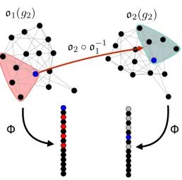
Figure 3: An illustration of the “label-independence” property of VN schemes. If the blue vertex in o₁(g2) (resp.,o2(g2)) is o1(u) (resp.,o2(u)) for u∈V2, then we require the ranks of I(o1(u);o1(g2)) (outlined in red in the network o1(g2) and colored red/blue in the ordering provided by Φ) to be equal to the ranks ofI(o₂(u);o₂(g2)) (outlined in grey in the network o₂(g2) and colored grey/blue in the ordering provided by Φ). Indeed, the set of ranks of o(I(u;g2)) via Φ is independent of the choice of obfuscation functiono.

Definition 11 (Vertex Nomination (VN) Scheme) For a set A, let TA denote the

set of all total orderings of the elements of A. For n, m > 0 fixed, obfuscating set W, and obfuscating function o ∈ O_W, a vertex nomination scheme is a function Φ : G_n×

o(Gm)×V1 → TW satisfying the following consistency property: If for each u ∈ V2, we

define rankΦ(g1,o(g2),v∗) o(u)

to be the position of o(u) in the total ordering provided by Φ(g1,o(g2), v∗), and we define rΦ :Gn× Gm×OW ×V1×2V2 7→2[m] via

r_Φ(g1, g2,o, v∗, S) ={rankΦ(g1,o(g2),v∗) o(u)

s.t. u∈S},

then we require that for any g1 ∈ Gn, g2 ∈ Gm, v∗ ∈V1, obfuscating functions o1,o2 ∈OW

and any u∈V(g2),

r_Φ g1, g2,o1, v∗,I(u;g2)

=r_Φ g1, g2,o2, v∗,I(u;g2)

(2)

⇔o2◦o−₁1

h

IΦ(g1,o1(g2), v∗)[k]);o1(g2)

i

=IΦ(g1,o2(g2), v∗)[k];o2(g2)

1 2 3 4 a b c d b a d c 1 2 3 4 a b c d b a d c

a. Well-defined scheme b. Not well-defined scheme

a b c d e b c e a d a b c d e b c e a d 1 4 2 3 5

a

b=e

c

d

b

c=d

e

a

a

b=e

c

d

b

c=d

a

e

1 2 3 4 a b c d b a d c 1 2 3 4 a b c d b a d c

a. Well-defined scheme b. Not well-defined scheme

a b c d e b c e a d a b c d e b c e a d

a

b=e

c

d

b

d

e=c

a

a

b=e

c

d

b

c

d

a

e

c. Not well-defined scheme Φ d. Not well-defined scheme

b. Not well-defined scheme Φ

d. Not well-defined scheme Φ

a. Well-defined scheme Φ

Φ

Φ

Φ

Φ

Φ

Φ

Φ

Φ

g

₂

g

2

g

2

g

₂ 1 4 2 3 5 1 4 2 3 5 1 4 2 3 5

O

₁

O

₁

O

₁

O

₁

O

₂

O

₂

O

₂

O

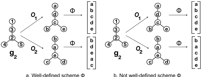
₂ a b c d e b d e a c a b c d e b a c d e

Figure 4: An example of the consistency criterion, Equation (2), in action. The left panel (a) shows a well-defined nomination scheme while the right panel (b) shows an ill-defined scheme. The key in this example is that any scheme satis-fying Equation (2) must have rΦ(g1, g2,o1, v∗,{1}) = rΦ(g1, g2,o2, v∗,{1});

r_Φ(g1, g2,o1, v∗,{3}) = rΦ(g1, g2,o2, v∗,{3}); rΦ(g1, g2,o1, v∗,{2}) =

rΦ(g1, g2,o2, v∗,{2}); and rΦ(g1, g2,o1, v∗,{4,5}) =rΦ(g1, g2,o2, v∗,{4,5}).

Given (G1, G2) ∼F_c,θ(n,m)∈ Nn,m realized asG1 =g1 and G2 =g2 withv∗ ∈V1 the vertex of interest inG1, a VN scheme Φ(·,·,·) produces a ranked list Φ(g1,o(g2), v∗) of the vertices ofo(g2) (i.e., the setW), ordered according to how likely each vertex inV(o(g2)) is judged to correspond tov∗, with optimal performance corresponding to

Φ(g1,o(g2), v∗)[1] =

(

o(v∗) ifv∗∈C

arbitrary v∈W ifv∗∈/ C.

Less formally, one can think of a VN scheme as ranking the vertices ofG2 according to how well they resemble the vertex of interestv∗ under some task-dependent measure.

Remark 12 Note that ifu∈V2 is such thatI(u;g2) ={u}(i.e.,uis topologically distinct within g2), then Equation (2) implies that

rank_{Φ(g1,o1(g2),v}∗₎ o₁(u)= rank_Φ(g

1,o2(g2),v∗) o2(u)

for anyo1,o2inOW. IfI(u;g2) contains vertices in addition tou, then Equation (2) implies

that the set of vertices topologically equivalent tou(namely, those inI(u;g2)) must achieve the same ranks via Φ under any two obfuscating functions; see Figure 4 for a simple example of this consistency criterion in action.

considered interesting precisely when they belong to one of K communities in a stochas-tic block model. While the two-graph VN formulation we consider in the present work (modulo symmetries) involves a single vertex of interest across graphs, the framework is easily extended to the setting where one may have multiple vertices of interest (and not of interest), and in particular it can encode instances of the one-graph version VN problem. To see this, consider an instance of the single-graph VN problem on graph G = (V, E) where V is partitioned into K communities as V = V1 ∪V2 ∪ · · · ∪VK and each of the

communities is comprised of labeled (i.e., seed vertices, whose community memberships are observed) and unlabeled (i.e., nonseed, whose community memberships are unobserved) vertices,Vk=Sk∪Uk, whereSk⊆Vkis the set of seeds from thek-th block andUk ⊆Vk is

the set of nonseed vertices. We can encode this one-graph VN instance as an instance of the two-graph problem by encoding additional information in the graphG1. Construct a vertex setV0 =V∪ {`1, `2, . . . , `K}. TheK new vertices{`k}Kk=1 will encode the label information present in the graph G. Let E0 = E∪L, where L = {{`k, s} : s ∈ Sk, k ∈ [K]}, so that

edges connect from seed vertices in S = S1 ∪S2∪ · · · ∪SK to their corresponding label

vertices. Take G1 = (V0, E0), and let the interesting vertices (and possible uninteresting vertices) be given by the elements of S ⊆ V0. The second graph G2 is then the subgraph of G induced by the unlabeled vertices U ⊆V passed through an appropriate obfuscating function. This pair (G1, G2), with anys∈S1 chosen to be the interesting vertex, encodes the label information present in the one-graph VN problem as well as the graph structure of G, as required.

3. Bayes Error and Bayes Optimality in Vertex Nomination

Viewing a VN scheme as an information retrieval system suggests that a scheme that puts

o(v∗) close to the top of the nomination list is potentially of great practical value, even if it fails to obtain perfect performance. Motivated by this, we adapt the recall-at-kmetric from classical information retrieval as a measure of performance. To wit, we define the level-k loss function and error for VN as follows.

Definition 14 (VN loss function, level-k error) Let Φ∈ Vn,m be a vertex nomination

scheme and oan obfuscating function. For (g1, g2) realized from (G1, G2)∼F_c,θ(n,m)∈ Nn,m

with vertex of interest v∗ ∈ C, and for k∈ [m−1], we define the level-k nomination loss via

`k(Φ, g1, g2,o, v∗) =1{rankΦ(g1,o(g2),v∗)(o(v

∗_{))≥k+ 1}}

= 1−1{rank_{Φ(g1,o(g2),v}∗₎(o(v∗))≤k}.

(3)

The level-kerror of Φ at v∗ is then defined to be

Lk(Φ, v∗) =E_(G

1,G2)∼F_c,θ(n,m)[`k(Φ, G1, G2,o, v

∗_)]

=P_(G

1,G2)∼F_c,θ(n,m)

rankΦ(G1,o(G2),v∗)(o(v

∗

From the definition of the level-kerror in Eq. (4), it is immediate that

L1(Φ, v∗) = 1−_P

(G1,G2)∼F_c,θ(n,m)

rankΦ(G1,o(G2),v∗)(o(v

∗_{)) = 1}

≥L2(Φ, v∗) = 1−P_(G

1,G2)∼Fc,θ(n,m)

rankΦ(G1,o(G2),v∗)(o(v

∗

))∈ {1,2}

≥L3(Φ, v∗) = 1−P_(G

1,G2)∼F_c,θ(n,m)

rank_{Φ(G1,o(G2),v}∗₎(o(v∗))∈ {1,2,3}

.. .

≥Lm−1(Φ, v∗) = 1−P_(G

1,G2)∼F_c,θ(n,m)

rankΦ(G1,o(G2),v∗)(o(v

∗_))∈[m−1]

, (5)

The level-1 loss function is analogous to the classical 0/1 loss function in classification, as L1(Φ, v∗) is simply the probability that Φ fails to “classify”o(v∗) as the vertex corresponding tov∗ ino(G2) (i.e., fails to rank it first). Considering 1 < km enables us to model the practical loss associated with using a VN scheme to search foro(v∗) ino(V2) given limited resources.

Remark 15 Unlike in the classification setting described in Section 1.2, whereLF(hn) is a

random variable indexed byn, the nomination errors defined in Definition 14 are sequences indexed by m and n and are not random. In the classical setting, LF(hn) denotes the

error rate of a classifier that classifies a single observationX based onn training instances {(Xi, Yi)}ni=1. In the case of VN, the notion of labeled training instances is, at best, more hazy. Indeed, in the present setting, the training data and test data are inseparable. The graphs (or, more specifically, their edges) are the training data, and in the present work, the graph orders n, m are better thought of as measuring problem dimension rather than training set size.

Analogous to the classification literature, we are now able to define the concept of Bayes optimality in the VN framework.

Definition 16 (Bayes error of a VN scheme) Let(G1, G2)∼F_c,θ(n,m) with vertex of in-terest v∗ ∈C (where we recall that C is the set of core vertices; see Definition 7), and let

o∈ OW be an obfuscating function. For k ∈[m−1], we define the level-k Bayes optimal

VN scheme to be any element Ψ ∈ arg minΦ∈Vn,mLk(Φ, v

∗_{), and define the level-k Bayes}

error to beL∗_k(v∗) =Lk(Ψ, v∗) for level-k Bayes optimal Ψ.

Now that we have a notion of Bayes error for VN, it is natural to ask whether an optimal VN scheme exists analogous to the Bayes optimal classifier of Equation (1). Toward this end, let (g1, g2) be realized from (G1, G2)∼Fc,θ(n,m)∈ Nn,m, and consider a vertex of interest

v∗ ∈C and obfuscating function o:V2 → W. In order to avoid the technical complexities associated with graph automorphisms, in what follows we will assume that F_c,θ(n,m)∈ Nn,m

is supported onGa

n× Gma, whereGna(resp.,Gma) is the set of asymmetric graphs inGn(resp.,

G_m). For analogous results in networks with symmetries, see Remark 18. Letting 'denote graph isomorphism, for (g1, g2)∈ Gn× Gm define the set

(g1,[o(g2)]) =

g1,˜g2

s.t. o(˜g2)'o(g2) =

g1,˜g2

s.t. ˜g2'g2 .

In order to define the Bayes optimal scheme, we will also need the following restriction of (g1,[o(g2)]): for eachw∈W,we define

(g1,[o(g2)])w=o(v∗₎=

n

g1,˜g2

s.t. ∃isomorphism σ s.t. o(˜g2) =σ(o(g2)), σ(w) =o(v∗)

o

. (7) We are now ready to define a Bayes optimal VN scheme.

For ease of notation, in the sequel we will write P_F(n,m)

c,θ

or even simply P in place of

P_(G

1,G2)∼F_c,θ(n,m) where there is no risk of ambiguity. Let

g=

n

g₁(i), g(₂i)oh

i=1 (8)

be such that the sets

n

g₁(i),[o(g(₂i))]oh

i=1 partition Ga

n× Gma. We will call this partition Pn,m, where we suppress dependence on g

and o for ease of notation. We will define a Bayes optimal scheme Φ∗ (independent of the choice of g) piecewise on each element of this partition, and we will prove in Theorem 17 that Φ∗ is level-kBayes optimal for allk∈[m−1]:

Φ∗

g(₁i),o(g(₂i)), v∗

[1]∈argmax

u∈W

P

h

g₁(i),[o(g(₂i))]

u=o(v∗₎

g(₁i),[o(g₂(i))]

i

Φ∗g(₁i),o(g(₂i)), v∗[2]∈ argmax

u∈W\{Φ∗_[1]}P

h

g₁(i),[o(g(₂i))]

u=o(v∗₎

g(₁i),[o(g₂(i))] i ..

.

Φ∗g(₁i),o(g₂(i)), v∗[m]∈ argmax

u∈W\{∪_j∈[m−1]Φ∗[j]}

P

h

g(₁i),[o(g₂(i))]

u=o(v∗₎

g₁(i),[o(g(₂i))] i, (9) with ties broken arbitrarily but deterministically. We refer the interested reader to Appendix B.1 for discussion of the case where ties are allowed in the ranking function. For each element

(g1, g2)∈

g(₁i),[o(g₂(i))]

\ng₁(i), g₂(i)

o

,

choose the permutation σ such that o(g2) =σ(o(g₂(i))), and define Φ∗(g(₁i),o(g2), v∗) =σ(Φ∗(g1(i),o(g

(i) 2 ), v

∗_)).

Lastly, the following theorem shows that this scheme (uniquely defined up to tie-breaking) is indeed Bayes optimal. A proof can be found in Appendix A.1.

Theorem 17 Let o∈OW be an obfuscating function, and let

g=ng₁(i), g(₂i)oh

i=1 be such that the sets

n

g₁(i),[o(g(₂i))]oh

partition Ga

n× Gma. Let Φ∗ = Φg∗ be as defined in Equation (9). Suppose that (G1, G2) ∼ F_c,θ(n,m)∈ Nn,m withF_c,θ(n,m) supported onGna× Gma, and consider a vertex of interestv∗ ∈C.

We have that Lk(Φ∗, v∗) = L∗k(v∗) for all k ∈ [m−1], partitions g, and all obfuscating

functions o.

Remark 18 The effect of symmetries on Theorem 23 is both subtle and cumbersome, as the specific tie-breaking procedures used in the analogue of Eq. (9) are of great import. To this end, consider g to be defined as above, and let T ∈ TW be the ordering that

speci-fies the (fixed but otherwise arbitrary) scheme by which elements within each I(v;o(g2)) are ordered. Informally, we will first rank the sets I(v;o(g2)) (rather than the individual vertices), and then use T to rank within and across each of the I(v;o(g2)). Full detail is provided below.

For each w∈W and v∈V(g2), define (g1,[o(g2)])I(w;o(g2))=o(v)=

n

g1,g˜2

s.t. ∃ iso. σ witho(˜g2) =σ(o(g2)), and σ(u) =o(v) for some u∈ I(w;o(g2))

o

.

(10)

As above, we will define the Bayes’ optimal VN scheme on each element of the partition provided viag. We first define a ranking Ψ of the sets

g₁(i),[o(g(₂i))]

I(u;o(g₂(i)))=o(v∗₎

indexed byu, and then will useT to give the total ordering from Ψ. To wit, for eachi∈[k], iteratively define (where ties in the argmax are broken in an arbitrary but nonrandom manner)

Ψ

g(₁i),o(g(₂i)), v∗

[1]∈ argmax

I(u;o(g₂(i)))⊂W

P

g₁(i),[o(g(₂i))]

I(u;o(g(₂i)))=o(v∗₎

g₁(i),[o(g(₂i))]

Ψg(₁i),o(g₂(i)), v∗[2]∈ argmax

I(u;o(g₂(i)))⊂W\{Ψ[1]}

P

g₁(i),[o(g(₂i))]

I(u;o(g(2i)))=o(v∗)

g₁(i),[o(g(₂i))]

.. .

Ψg(₁i),o(g₂(i)), v∗[`]∈ argmax

Io(g₂₎(u)⊂W\{∪`j−=11Ψ[j]}

P

g₁(i),[o(g(₂i))]

I(u;o(g₂(i)))=o(v∗₎

g(₁i),[o(g₂(i))]

.

(11) For each element

(g1, g2)∈(g (i) 1 ,[o(g

(i)

2 )])\ {(g (i) 1 , g

(i) 2 )}, choose an isomorphismσ such thato(g2) =σ(o(g2(i))), and define

Ψ(g1,o(g2), v∗) =σ(Ψ(g1(i),o(g (i) 2 ), v

∗_)).

For each (g1, g2)∈ Gn× Gm, we define a VN scheme Φ∗T from Ψ as follows:

1. Initialize Φ∗_T(g1,o(g2), v∗) as an empty list; initialize j = 1;

2. If Ψ(g1,o(g2), v∗)[j] is nonempty, add the top ranked (according to T) element from Ψ(g1,o(g2), v∗)[j] to the end of Φ∗T(g1,o(g2), v∗), else do nothing; set j = j + 1 (mod |Ψ(g1,o(g2), v∗)|)

3. Repeat Step 2 until there are no more vertices to add to Φ∗_T(g1,o(g2), v∗).

If T[1] =o(v∗), then Φ∗_T(g1,o(g2), v∗) is Bayes optimal (as in Theorem 17) in the sense of Definition 16. See Appendix A.1 for details.

Example 1, continued. Let (G1, G2) ∼ R-ER(P) for P, R ∈ Rn×n. Under mild model assumptions, we have that limn→∞L∗_k(v∗) = 0 for any fixedk. This is due to the fact that

the optimal graph matching ofG1 too(G2) will almost surely recover the true vertex labels of o(G2) for nsuitably large; i.e.,

argmin_Q∈ΠnkAQ−QBk_F ={In}with probability→1,

where Πn is the set ofn×n permutation matrices, A is the adjacency matrix for G1 and B the adjacency matrix for G2. More concretely, we have the following theorem adapted to our present setting from Lyzinski and Sussman (2018). A proof sketch can be found in Appendix B.

Theorem 19 Let (A, B) ∼R-ER(P), and for any fixed permutation matrix Q define the random variableδ(Q) :=kAQ−QBk_F. Define 0< := mini,j;i6=j2Ri,jPi,j(1−Pi,j). There

exist positive constants c1, c2 such that if 2> c1log(n)/n, then for sufficiently large n, P(∃ Q∈Πn\ {In} s.t. δ(Q)≤δ(In))≤2 exp

−c22n .

Similarly to the Bayes optimal scheme, we define the graph matching VN scheme, denoted ΦM, separately on each element of Pn,n. For a given (˜g1,[o(˜g2)]) ∈ Pn,n,let (g1, g2) be an fixed element in (˜g1,[o(˜g2)]). Define ΦM(g1,o(g2), v∗)[1] to be a fixed but arbitrary element from

r−1(v∗) s.t. Qr∈argminQ∈ΠnkAQ−QBkF , (12)

where each r :W → V2 appearing above is a bijection and Qr its associated permutation matrix (having identified bothW andV2 with the set [n]). Define

R₁=nr:W →V2 s.t. r is a bijection withr−1(v∗) = ΦM(g1,o(g2), v∗)[1]

o

.

Ifj >1, define ΦM(g1,o(g2), v∗)[j] to be any element of

n

r−1(v∗) s.t. Qr∈ argmin

Q∈Π(n)\{Qr:r∈Sj<sub>`=1</sub>−1R`}

kAQ−QBk_Fo,

whereRj is defined analogously toR1. For each element (g01, g20)∈(˜g1,[o(˜g2)])\ {(g1, g2)}, choose a permutation σ such thato(g₂0) =σ(o(g2)), and we then define ΦM(g1,o(g20), v∗) = σ(ΦM(g1,o(g2), v∗)).Theorem 19 states that under mild model assumptions, we have that ΦM(G1,o(G2), v∗)[1] =o(v∗) asymptotically almost surely, and thus limn→∞L1(ΦM, v∗) =

that limn→∞L∗_k(v∗) = 0 in this model for any fixed k.

The next two examples serve to illustrate how the level-k Bayes error behaves in the presence of stochastically indistinguishable vertices. In essence, we cannot hope to perform better than randomly ordering stochastically equivalent vertices.

Example 3, continued. Let G1 and G2 be independent ER(n, p) graphs. Since the vertices are stochastically indistinguishable within each of the two graphs, no nomination scheme can do better than random chance in this model. Thus, withc =n, we have that L∗_k(v∗) = (1−k/n)(1 +o(1)) for all k∈[n−1] and all v∗∈[n].

Example 4 Letp1, p2, q∈[0,1] with 1≥p1> p2 ≥0 andq 6=p1, p2. Define the matrix

B =

p1 q q p2

,

and let G1, G2 be independent SBM (2, B, bn) graphs where bn(i) = 1 if i ≤n/2 (n even)

andbn(i) = 2 ifi > n/2. Withc=nand the correspondence equal to the identity function,

let (kn)∞n=2 be a nondecreasing divergent sequence satisfying kn ≤ n/2 for all n >1, then

limnL∗kn(v

∗_{) = lim}

n[(1−2kn/n)∨0] for allv∗. Indeed,L∗kn is asymptotically equivalent to randomly ordering then/2 vertices inG2 that are stochastically equivalent tov∗.

4. VN Consistency

With the definition of Bayes optimality and the Bayes optimal scheme in hand, it is now possible to define a notion of consistent vertex nomination analogous to consistent clas-sification in the pattern recognition literature. Before defining a consistent VN rule (i.e., a sequence of VN schemes), we must first define the notion of sequences of nominatable distributions with nested cores. Such sequences of distributions are necessary in order to speak sensibly of a sequence of vertex nomination problem instances.

Definition 20 Let F = F_c(n,mn) n,θn

∞

n=n0 be a sequence of distributions such that F

(n,mn)

cn,θn ∈ Nn,mn for all n. We say thatF has nested cores if for alln0≤n1< n2, if

(G1, G2)∼Fn1 =F

(n1,mn₁)

cn1,θn1 and (

e

G1,Ge2)∼F_n2 =F

(n2,mn₂)

cn2,θn2 ,

we have, letting C1 and C2 be the core vertices associated with Fn1 and Fn2 respectively,

and denoting the junk vertices J1,1, J2,1, J1,2,Je_2,2 analogously,

[i.]V(G1) =C1∪J1,1⊂V(Ge1) =C₂∪J_2,1;

[ii.] V(G2) =C2∪J1,2 ⊂V(Ge2) =C₂∪J_2,2;

[iii.]C1 ⊂C2.

We are now ready to define a consistent VN rule.

Definition 21 Let

F=Fn=Fc(nn,m,θnn)

∞

be a sequence of distributions such thatFn∈ Nn,m(n)with nested cores satisfyinglimn→∞mn=

∞. For a given non-decreasing sequence (kn), we say that a VN rule Φ= (Φn,mn)

∞

n=n0 is

level-(kn) consistent at v∗ with respect to Fif

lim

n→∞Lkn(Φn,mn, v ∗

)−L∗_kn(v∗) = 0,

for any sequence of obfuscating functions of V2 with |V2| = mn. If a rule Φ is level-(kn)

consistent at v∗ for a constant sequence kn=k, n= 1,2, . . ., then we say simply that Φis

level-k consistent.

Remark 22 Equation (5) has an interesting implication for VN consistency in the setting where L∗_kn(v∗) → 0. In this case, level-(kn) consistency of a VN rule Φ implies that Φ is

(k0_n)-consistent for all (k_n0) such that lim inf kn0

kn ≥ 1. We conjecture that this implication holds true for the case where L∗_k

n(v

∗_{)→c >0, but this problem remains open at present.}

Example 1, continued. Let F = (F_n,θ(n,n_n=() _P

n,Rn)) be a sequence of Rn-ER(Pn) random graph models in Nn,n for some sequence of probability matrices (Pn)∞n=n0 and correlation

matrices (Rn)∞n=n0. Under mild model assumptions (see Theorem 19), the graph matching

vertex nomination rule ΦM defined in Equation (12) above is level-1 consistent, and hence

level-(kn) consistent for all (kn) sequences.

Example 3, continued. Let F = (F_n,θ(n,n_n=)_p) be a sequence of independent ER(n, p) ran-dom graph models in N. All vertex nomination rules are level-(kn) consistent for all (kn)

sequences. This holds for all possible values of c ∈ [n] in the nested sequence of ER(n, p) distributions, as all VN rules have effectively chance performance, regardless of core size under this model.

We define the consistency of a VN rule with respect to a broad class of graph sequences, and it is perhaps no surprise that there cannot be any level-(kn) universally consistent VN

rules. Indeed, even for constant sequenceskn:=k (i.e., those that are level-(kn) consistent

Theorem 23 Letnandmbe large enough to guarantee the existence of asymmetric graphs g1 ∈ Gn and g2 ∈ Gm. Consider a VN scheme Φ ∈ Vn,m, obfuscating function o, and

strictly increasing sequence (i)mi=1 satisfying i ∈ (0,_mi ). Then there exists a distribution

F_c,θ(n,m)∈ Nn,m over Gn× Gm and v∗∈C such that for each k∈[c−1],

L∗_k(v∗)≤m−k<1−

k

m <1−k < Lk(Φ, v

∗

),

where1−_mk represents the error probability of chance performance, i.e., the error probability of a VN scheme in the independent Erd˝os-R´enyi setting.

In the remainder of the section, we will suppress the dependence ofm=mnonn. If we

consider sequences (m,i)mi=1 satisfying the assumptions of Theorem 23 and limnm,m−kn = ∈(0,1) for a given (kn) satisfyingkn=o(m), we arrive at the following Corollary, namely

that level-(kn) universally consistent VN schemes do not exist for any sequence (kn)∞n=n0

that does not grow as fast as m=|V(G2)|.

Corollary 24 Let ∈ (0,1) be arbitrary, and consider a VN rule Φ = (Φn,m). For any

nondecreasing sequence (kn)∞n=n0 satisfying kn =o(m), there exists a sequence of

distribu-tions (F_c,θ(n,m)∈ N_n,m)∞_n=n0 with nested cores such that lim sup

n→∞L ∗

kn(v

∗_{) = <1 = lim}

n→∞Lkn(Φn,m, v ∗_).

Corollary 24 has a number of practical implications. Below, we will briefly outline two such implications. Unlike in the classification setting, where universally consistent rules (e.g., k-nearest neighbors) are theoretically guaranteed to perform well in big-data settings, the VN practitioner enjoys no such certainty. Indeed, in VN, the practitioner first needs to identify the consistency class of a VN rule (i.e., the set of models for which the VN rule is consistent) before applying it in real settings. Unfortunately, identifying and enumerating these consistency classes is theoretically and practically nontrivial, and we are investigating theory and heuristics for this at present. In a streaming data setting, the performance of a universally consistent classifier will approach Bayes optimality for the distribution governing the data, and the classifier will be guaranteed to successfully adapt itself to any changes in the underlying data distribution. The lack of universal consistency in the VN setting implies that his is not the case for graph data, as the performance, as the performance of a consistent VN scheme in the streaming setting could precipitously decline in the presence of distributional shifts in the data. Recognizing these shifts and their potential impact on VN performance is paramount and is the subject of current research.

4.1. Global Consistency

world networks, but, as we will demonstrate below, restricting our model class to sim-pler dependency structures still does not necessarily guarantee the existence of universally consistent schemes.

It is thus natural to explore a weaker notion of consistency, namely consistency for a sufficiently large family of nominatable sequences rather than for all nominatable sequences.

Definition 25 Let

F=

Fα =

F_c(n,mn),α n,θn

∞

n=n0

:α∈ A

be a family of nominatable sequences, indexed by some set A. We say that VN schemeΦis level-(kn) F-globally consistent if Φ is level-(kn) consistent for every F∈F. We call such

a family level-(kn) globally consistent.

The question of the maximal familyFfor which a level-(kn)F-globally consistent rule exists

is of prime interest. While we cannot offer a satisfactory complete answer to that question in the present work, we do offer some examples of globally consistent families.

Example 1 continued: In settings where corresponding vertices have correlated neighbor-hood structures across networks, there is hope for finding globally consistent rules. In the ongoing Example 1, we have seen a simple example of this in theR-ER(P) model, in which the matrix of correlationsRencodes a correspondence across the two graphs. As mentioned previously, Theorem 19 asserts that under some mild model assumptions onR andP in the R-ER(P) model, level-1 globally consistent VN rules exist (namely the graph matching VN scheme). If F denotes the set of distributions obeying these model assumptions, then we have that level-(kn)F-globally consistent rules exist for all sequences (kn). While we do not

expect the conditions of Theorem 19 to produce a maximal level-(kn) globally consistent

family for any given (kn), this example nonetheless provides an important intuition for the

properties such maximal families might possess.

Example 4 continued: The SBM provides a prime example of global consistency. Working in the one-graph framework of Remark 13, under appropriate growth conditions on the parameters of every sequence in family F, Theorem 6 in Lyzinski et al. (2016) implies the existence of a likelihood-based nomination scheme that is level-(|U1|) globally consistent for this family of models. Under similar growth conditions, Theorem 6 in Lyzinski et al. (2014) implies the existence of a level-(|U1|) globally consistent scheme based on spectral clustering, in which vertices are nominated based on their proximity to the vertex or vertices of interest.

Remark 26 An attempt at systematically constructing a maximal globally consistent fam-ily might begin by putting model restrictions onto elements ofN_n,m. A natural restriction to consider would be to demand that the models in F be nested in the following sense: For F ∈ F, if (G1, G2) ∼ F

(n2,mn₂)

cn₂,θn₂ with n1 < n2, then (G1

[n1]

, G2

[mn1]

) = (L G0₁, G0₂) where (G0₁, G0₂)∼F(n1,mn1)

cn₁,θn₁ . This property would allow us to consider “streaming” network modelsF, where forn1< n2, if (g1, g2) is realized from (G1, G2)∼F

(n2,mn2)

cn₂,θn₂ , and (g

0

1, g02) is realized from (G0₁, G0₂)∼F(n1,mn1)

n2−n1 vertices to (g01, g20). Additionally, this would serve to mimic the nested nature of the data in the classification consistency literature. However, as we will see in Example 5, global consistency depends both on the dependency structure within each graph (as seen in Theorem 23)and the vertex correspondence (i.e., the potential dependency structure across graphs) encoded in the model.

4.2. Behavioral (In)consistency and Global (In)consistency

We suspect that if the vertices of interest have a common distinguishing probabilistic and/or topological characteristic (e.g., correlated neighborhoods, common SBM block structure, high network centrality, etc.) then a globally consistent rule may exist. Indeed, under mild model assumptions, this is the case in theR-ER(P) of Example 1; in the i.i.d. SBM of Example 4 where the correspondence is the identity function (Lyzinski et al., 2014); and in the i.i.d. ER of Example 3, to name a few. In each of these examples, there is a stochastic/topological similarity (or in the ER case, uniformity) between corresponding vertices across networks. In each, corresponding vertices behave similarly across networks. While we suspect that this behavioral similarity is not sufficient for global consistency, Example 5 demonstrates that behavioral inconsistencies within a family of nominatable distributions can preclude the existence of globally consistent nomination rules.

Example 5 For eachn, considern-vertex random graphsG1∼asym-SBM(2, B1, b(1)n )

inde-pendent ofG2∼asym-SBM(2, B2, b(2)n ), where asym-SBM denotes the stochastic blockmodel

distribution restricted to have support on asymmetric graphs. This restriction is made to avoid the unpleasantries of symmetries, and is asymptotically negligible as the SBMs con-sidered in this example are asymptotically almost surely asymmetric.

Case 1. In this case, corresponding vertices behave similarly across networks. To wit, let F= (Fn)∞n=n0 be the sequence of models where

B1 =B2=

p1 q q p2

, b(1)_n (i) =b(2)_n (i) =

(

1 ifi≤n/2;

2 ifi > n/2,

p1 6=p2,c =n, and the correspondence is the identity function. As stated before, in this model L∗_n/2(v∗) →0 for allv∗ ∈C. Without loss of generality, considerv∗ =v1 =u1 = 1. IfΦis consistent with respect to F then

PFn(rankΦ(G1,o(G2),v1)(o(u1))≥n/2 + 1)→0.

By the distributional equivalence of vertices within the same block, and the consistency property in the definition of a VN scheme, for any u, v∈b−_n1(1), k∈[n] we have that

PFn(rankΦ(G1,o(G2),v1)(o(u)) =k) =PFn(rankΦ(G1,o(G2),v1)(o(v)) =k).

Letting this common value be set to αk,n (with βk,n defined similarly as the common value

of PFn(rankΦ(G1,o(G2),v1)(o(u)) =k) for uin block 2), we have that

n X

i=1

PFn(rankΦ(G1,o(G2),v1)(o(ui)) =k) = 1 =

n(αk,n+βk,n)

giving us thatαk,n= 2/n−βk,n. Consistency implies that

n/2

X

k=1

αk,n→1,

which implies that

n/2

X

k=1 αk,n =

n/2

X

k=1

(2/n−βk,n) = 1− n/2

X

k=1

βk,n →1,

implying Pn/_k=12 βk,n→0.Therefore, for any u in block 2,

PFn(rankΦ(G1,o(G2),v1)(o(u))≥n/2 + 1)→1.

Case 2. In this case, corresponding vertices behave differently across networks. To wit, let ˜

F= ( ˜Fn)∞n=n0 be the sequence of models where

B1=

p1 q q p2

, B2 =

p2 q q p1

, b(1)_n (i) =b(2)_n (i) =

(

1 ifi≤n/2; 2 ifi > n/2,

c=n, and the correspondence is the identity function. As in Case 1 considered above, in this model L∗_n/2(v∗) → 0 for all v∗ ∈ C, and, as above, consider v∗ = v1 = u1. If Φ is consistent with respect toF˜ then

P_F˜_n(rankΦ(G1,o(G2),v1)(o(u1))≥n/2 + 1)→0.

Note that ifσ is the permutation such that

σ(i) =

(

i+n/2 ifi≤n/2;

i−n/2 ifi > n/2,,

thenPFn(g1, g2) =P_F˜_n(g1, σ(g2)). Define

En={(g1, g2) s.t. rankΦ(g1,o(g2),v1)(o(u1))≥n/2 + 1}}

i.e., and ˜En={(g1, g2) s.t. (g1, σ(g2))∈En}, i.e.,

˜

En={(g1, g2) s.t. rankΦ(g1,o(g2),v1)(o(un/2+1))≥n/2 + 1}.

IfΦis consistent with respect to Fwe have thatPFn(En)→0 which implies (as (g1, g2)∈ En⇔(g1, σ(g2))∈E˜n)P_F˜_n( ˜En)→0. IfΦis consistent with respect toF˜thenP_F˜_n(En)→0

and P_F˜_n( ˜En) → 1. We arrive at a contradiction, and Φ cannot be (n/2)-consistent with

Although Example 5 may seem artificial, it is a simple representation of a common phenomenon observed in network data. Often the same entity can behave quite differently across networks; see Patsolic et al. (2017) for an example of this in social networks and Chen et al. (2016b) for an example of this in connectomics. In such a setting, intuition says that a universal scheme that works in both behavioral settings should not exist. Indeed, at least in the simple block model setting considered above, we see that no such scheme exists. Example 5 also highlights an important difference between the VN setting and the more standard classification framework. We already noted that classification’s universal consistency relies on the distribution not changing in n, whereas in VN the distributions must vary with n (indeed, the graph sizes grow inn). Further, Example 5 shows that the nonexistence of a universally consistent scheme is not simply a consequence of changing the underlying distributional parameters with n, as these two SBM distributions are (essen-tially) fixed, in that the matrix B does not change with n. In this example the “training data” provided byG1 cannot be uniformly beneficial for a single VN scheme across the two differing model settings we consider. Contrast this with the classification setting of Devroye et al. (1997), where the training data uniformly provides progressively better estimates of the class-conditional distributions. Indeed, the training data helps delineate potentially interesting vertices from non-interesting ones in G2 in Case (1) for one VN scheme, and in Case (2) for another VN scheme, but there does not exist a VN scheme that achieves this desired class separation across both cases.

Remark 27 In the cases considered in Example 5, if we introduce positive edge-wise correlation of

ρ≤

s

min

p1(1−p2) p2(1−p1)

,p2(1−p1) p1(1−p2)

into both Case 1 and Case 2, then under mild assumptions on the growth ofp1 andp2, joint consistency can be recovered via a USVT centered graph matching nomination scheme (see Lyzinski and Sussman, 2018, for details). This example demonstrates that it is sometimes possible to toggle a family of models to allow for global consistency. A note of caution is needed, however, as in this particular example the correlationρ is introducing a behavioral consistency across networks that addresses the precise issue brought forth by the behavioral inconsistency in Example 5. In other, more nuanced model families, we do not expect the global-consistency modification (if it indeed exists) to be as straightforward as adding additional edge-correlation into the model.

4.3. Vertex Nomination on Networks with Node Covariates

It is natural to ask if incorporating vertex features into the VN framework can resolve the lack of universally consistent VN schemes. While straightforward to implement, the ameliorating effect of features is significantly more nuanced. Before defining the VN scheme with features, we need the following extension of I(v;g) forg ∈ G_n and v∈V(g). Letting X be the space of vertex features for graphs in Gn, for g ∈ Gn, v∈ V(g), and X ∈ Xn we

define

e

I(v;g, X) ={u∈V(g) :∃automorphism τ of g s.t. τ(v) =u and Xu =Xv},

Definition 28 (Vertex Nomination (VN) Scheme with features) Let X (resp., Y) be the space of vertex features of graphs in Gn (resp., Gm). Forn, m >0 fixed, obfuscating

set W and obfuscating function o ∈ O_W, a vertex nomination scheme with features is a function

Φ :Gn× Xn×o(Gm)× Ym×V1 → TW

satisfying the following consistency property: If for each u∈V2, we define rank_{Φ(g1,X,o(g2),o(Y),v}∗₎ o(u)

to be the position of o(u) in the total ordering provided byΦ(g1, X,o(g2),o(Y), v∗), and we define r_Φ :G_n× Xn_{× G}

m× Ym×OW ×V1×2V2 7→2[m] via

r_Φ(g1, X,o(g2),o(Y), v∗, S) ={rankΦ(g1,X,o(g2),o(Y),v∗) o(u)

s.t. u∈S},

then we require that for any g1 ∈ Gn, g2 ∈ Gm, v∗ ∈ V1, X ∈ Xn, Y ∈ Ym, obfuscating functions o1,o2 ∈OW and any u∈V(g2),

r_Φ g1, X,o1(g2),o1(Y), v∗,I(e u;g₂, Y)

=r_Φ g1, X,o2(g2),o2(Y), v∗,Ie(u;g₂, Y)

. (13)

We let Ve_n,m denote the set of all such VN schemes.

It is immediate that if the features are sufficiently informative, consistency can be estab-lished with features where it could not be without. Indeed, consider in Example 5 features that encode the community memberships of a few vertices (e.g., a few vertices whose cor-respondences across the two graphs are known a priori). Combined with spectral methods, these would be sufficient for consistent VN under either behavior regime. It is also immedi-ate that the fundamental idea presented in Example 5 has an analogue when vertex features are available, as illustrated by the following example.

Example 6 For each n, considern-vertex random graphs G1∼asym-SBM(3, B1, b(1)n )

in-dependent of G2∼asym-SBM(3, B2, b(2)n ), where asym-SBM again indicates the stochastic

block model with support restricted to the asymmetric graphs.

Case 1. In this case, corresponding vertices behave similarly across networks. To wit, let F= (Fn)∞n=n0 be the sequence of models where 3|nand

B1 =B2 =





p1 q q q p2 q q q p2



, b(1)_n (i) =b(2)_n (i) =   

 

1 ifi≤n/3; 2 ifi∈(n/3,2n/3]

3 ifi > n/3,

p1 6=p2,c=n, the correspondence is the identity function, andv∗= 1 is in block 1. Case 2. In this case, corresponding vertices behave differently across networks. To wit, let F= (Fn)∞n=n0 be the sequence of models where 3|nand

B1 =





p1 q q q p2 q q q p2



, B2 =





p2 q q q p1 q q q p2



, b(1)_n (i) =b(2)_n (i) = 

 

 

1 ifi≤n/3; 2 ifi∈(n/3,2n/3]

p1 6=p2,c=n, the correspondence is the identity function, andv∗= 1 is in block 1. Similar to Example 5, without features no VN scheme can be (n/3)-consistent for both Cases 1 and 2 simultaneously. In a similar fashion, if we consider featuresX andY defined via

Xv =Yv= (

1 ifb(1)(v) = 1 −1 ifb(1)_{(v) = 2,3,}

then joint consistency is achievable for both Cases 1 and 2, for example by relying on features and ignoring graph structure. However, if we consider features X and Y defined via

Xv =Yv = (

1 ifb(1)(v) = 1,2 −1 ifb(1)_{(v) = 3,}

then joint consistency is again not achievable for both Cases 1 and 2 simultaneously.

This example demonstrates that features, in general, are not enough to ensure universal consistency. Nevertheless, insofar as features supply additional information, they have the potential to improve VN performance. A more thorough examination of the effect and effectiveness of vertex features in VN is beyond the scope of this work, and is the subject of current research.

5. Discussion