189 *Corresponding author
email address: [email protected]
M. R. Nikpoura, P. Khosraviniab,* and D. Farsadizadehc
a
Department of Water Engineering, University of Mohaghegh Ardabili, Ardabil, Iran
b Department of Water Sciences and Engineering, University of Kurdistan, Sanandaj, Kurdistan, Iran c Department of Water Engineering, University of Tabriz, Tabriz,East Azerbaijan, Iran
Article info: Abstract
Formation of shock waves has an important role in supercritical flows studies. These waves often occur during passage of supercritical flow in the non-prismatic channels. In the present study, the effect of length of contraction wall of open-channel for two different geometries (1.5 m and 0.5 m) and fixed contraction ratio was investigated on hydraulic parameters of shock waves using experimental models (models 1 and 2). For achieving to this goal, values of height and instantaneous velocity were measured in various points of shock waves observed in contractions for four Froude Numbers. In general, non-uniform distribution of velocity and turbulence intensity profiles were completely clear. Comparing the results of models 1 and 2 shows that the height and velocity values of formed waves in the model 2 is so much more than that of model 1. Also, motion of the shock waves was accompanied with longitude gradient decrease of turbulence kinetic energy. The results of the present research can be very useful for design engineers.
Received: 11/11/2016
Accepted: 18/08/2018
Online: 26/08/2018
Keywords:
Contraction,
Shock wave,
Supercritical flow,
Turbulence intensity,
Turbulence kinetic energy.
Nomenclature
u Instantaneous velocity component in the
x- direction
u
Average velocity component in thex-direction
1
u Average of flow velocity beneath the
sluice gate
X Longitude distance at the beginning of
wave formation
z Vertical distance from the bed
d Opening of sluice gate
Q Flow discharge
H Flow head
y Water depth
Fr1 Froude number for incoming flow
K Water depth
'
u Minor fluctuation of instantaneous
velocity
Abbreviations
CSW Classic shallow water equations
ECSW Extended classic shallow water equations
CFD Computational fluid dynamic
VOF Volume of fluid
1. Introduction
190
hydraulic engineering applications. Along the peak flows, the supercritical flow can be observed in most of the natural channel such as rivers and mountainous streams [1]. Compared to subcritical flow, supercritical open channel flow is characterized by the formation of shock waves [2].
The transverse waves generated in fast flows of open channels are similar to shock waves in supersonic gases. Therefore, the transverse waves formed in supercritical flows are also known as shock waves. The presence of complications such as constriction, expansion, rising and lowering of bed level, bends, and etc. in channels with supercritical flow situations, will cause a sudden change in the depth and velocity of the flow and subsequently, the shock waves can form. In the study of supercritical flows, the formation of shock waves is of high importance. Based on the change cross-section geometry obstacle, within the flow area and deflection of the side wall, the shock wave can be generated in the supercritical flow situation. This issue can damage the hydraulic structure and the surrounding environment [3]. In a contraction, production of the shocks generates a disturbance pattern that can persist for a considerable distance downstream. However, if the transition is designed properly, the waves will not propagate in the downstream channel. It is necessary to estimate the location of oblique standing wave and the elevation of the water surface in order to design wall heights against over tapping [4]. For the first, Von-Karman (1938) was able to derive the governing two-dimensional of supercritical flow in contractions using the CSW [2]. The analytical solution for the wave development in straight transitions was provided by Chow (1959) [5]. In recent years, advanced numerical methods have been applied for studying shock waves in transitions. The unsteady, depth-averaged and two-dimensional shallow water equations to simulate transient free-surface flow under extreme boundary situations have solved using the finite difference method [6-7]. In order to predict different properties of the flow situation, the suitability of the numerical methods is demonstrated in their studies. Analysis of shallow water equations was carried out for numerical simulation of
supercritical flow in sharp bends [8]. Analyzing flow profiles was done in subcritical and supercritical flows in an open channel that included either a contraction in width or a rise in the bottom using the specific-energy concept [9]. The CSW equations were extended. For simulating supercritical flow (i.e. Froud number equals 8), the CSW equation, based on modified Rouse channel expansion, was extended. It should be noted that the experimental studies were done by Mazumder and Hager (1993) [10]. It should be noted that the experimental studies were done by Mazumder and Hager (1993) [11]. The results of the extended method (ESWE) were compared with the experimental data and standard SWE. In order to estimate the free surface of supercritical flow in gradually open channel expansions, a 3-D CFD model was applied [12]. The comparison result of surface flow profile and shock front wave revealed that the numerical and experimental results have the satisfactory agreement. For estimating the supercritical bend flow in a rectangular chute, an analytical model was developed [13]. The suggested model was tested by comparing the results with the experimental data and obtained theoretical equations of the free surface profile. By adding a convex corner to the inner bend wall, a new approach was developed for the reduction of wave height through the outer wall of bend [14]. The wave height can be reduced as 10-45%, using an optimized convex corner. Supercritical flow in curved open channels was simulated using three-dimensional CFD analysis [15]. The CFD analysis was carried out on two 45° curved open channels using the FLUENT. Overall results indicated that the model has an excellent prediction of flow pattern of supercritical bend flow and also the wave length and height in the inner and outer wall of bends. The complex flow pattern occurring in a closed conduit bend with supercritical flow situation was reported. They developed a simple empirical relationship that describes the effects of the bend deflection angle and approachs flow situations on the considered flow [16].
191 simulation, two distinct models including
Reynolds- averaged Navier–Stokes equations (RANS) with the k-e turbulence model and the Shallow Water Equations (SWEs) were utilized. Comparison results in good agreement between numerical simulation and observed data [17]. The capability of a coupled 1D-2D model to simulate the flow processes during supercritical flows in crossroads was studied. They stated that the coupled 1D-2D model can be useful for reducing running time while preserving the solution accuracy and level of detail [18]. On the base of literature and to the best of the authors' knowledge, although the free surface profile in contraction was investigated, analysis of turbulence parameters has not been considered at the contraction location. In the present study, values of depth and instantaneous velocity were measured in various points of shock waves observed in contractions for four Froude numbers. In addition to analyzing free surface and velocity profiles, turbulence parameters of shock waves including turbulence kinetic energy and turbulence intensity were investigated.
2. Materials and methods 2. 1. Experimental setup
The experiments of this research were conducted in the hydraulic laboratory at the University of Urmia, Department of Water Engineering. The test facility comprised of a horizontal 6.0 m long, 0.7 m high and 1.0 m wide rectangular metal flume. A head tank with a length of 1.75 m, height of 1.20 m and width of 1.65 m supplied the discharge into the flume. The entrance discharge to the reservoir was set by a valve installed on the drift tube of a pump. A steel sluice gate with a thickness of 3 mm and a height of 2.1 m was installed at the entrance of the flume in order to regulate the water level and control the Froude number. During the tests, four sheets of plexiglass with a thickness of 6 mm, length of 1 m and height of 30 cm were utilized to make upstream and downstream channels of transitions. Also, four sheets of plexiglass with a thickness of 6 mm, length of 1.5 and 0.5 m and height of 30 cm were utilized for walls of the transitions. A false floor made of compressed
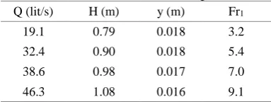
polyethylene with a thickness of 1 cm, length of 3.5 m and width of 1 m was placed at the beginning of the flume, in order to install walls of the transitions, upstream and downstream channels. In all experiments, the opening of sluice gate was 2 cm and widths of the upstream and downstream channels were considered 80 and 40 cm, respectively. The flow discharges were measured by an ultrasonic flow-meter having the accuracy of 0.02 lit/s. The wave heights in the section of contractions were measured at equally spaced intervals by a point gauge having the accuracy of 0.1 mm. An electromagnetic 2-D velocity meter was used for measuring of instantaneous velocity in various points of shock waves. The experiments were conducted for four Froude numbers including 3.2, 5.4, 7.0 and 9.1. It should be noted that the Froude number during the experiments were obtained by changing the water level in the tank head. Important flow parameters are listed in Table 1, where Q, H, y, and Fr1 are referred to the discharge, flow head, water depth, and Froude number for incoming flow, respectively.
Table 1. Characteristics of the experiments. Fr1 y (m)
H (m) Q (lit/s)
3.2 0.018
0.79 19.1
5.4 0.018
0.90 32.4
7.0 0.017
0.98 38.6
9.1 0.016
1.08 46.3
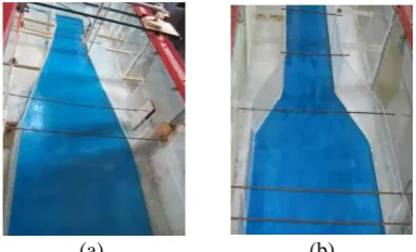
In order to investigate the effect of transition wall length on hydraulic parameters of the shock waves, two models of the contractions were used with straight walls and lengths of 1.5 and 0.5 m (model 1 and model 2). Fig. 1 shows a view of the contractions used in this study. After stabilizing the water level in the head tank for the Froude numbers in Table 1, with water passing under the sluice gate, supercritical flow was seen within the channel. Upon reaching the supercritical flow to the beginning of the transition, the shock waves start in diagonal form and collide with each other.
192
(a) (b)
Fig. 1. Upstream view of the contractions; (a) model 1 and (b) model 2.
Fig. 2. Formation of the shock waves in the model 1 for Fr1 = 7.0.
Fig. 3. Formation of the shock waves in the model 2 for Fr1 = 7.0
After reaching a steady flow situations and stability of wave’s pattern in the contractions, values of instantaneous velocity were measured by the velocity meter along the wave’s front in a distance of 10 cm from the beginning of the wave generation in five sections spaced 30 cm in length and 10 cm in the models 1 and 2. In addition, in the model 1, the values of velocity were measured in the vertical direction from a distance of 5 mm of the bed to 5 mm of the wave’s surface at intervals of 5 mm, vertically. For instance, the locations of instantaneous velocity measurements for model 2 are shown in Fig. 4.
Fig. 4. The locations of instantaneous velocity measurements for model 2.
In the same way, in the model 2, they were measured in a vertical direction from a distance of 5 mm of the bed to 1 cm of the wave’s surface at intervals of 5 mm. Velocity values were measured for 5 S at any point of the waves. 100 components of instantaneous velocity (u) were recorded within that time, and the average of them was considered for the target point (u). As mentioned, surface profiles of the shock waves were measured by the point gauge along the wave’s front. Due to the high intensity of flow turbulence and mixing of water and air, there was a risk of error when reading the wave surface profiles. In order to minimize the error,
the height was measured at
each point for several times, and the average of them was recorded as wave height of the target point.
3. Results and discussion
3. 1. Analysis of height and velocity profiles of shock waves
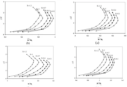
Figs. 5 and 6 show the velocity profiles of models 1 and 2 along the shock waves movement for the Froude numbers. X(m) demonstrates longitude distance at the beginning of wave formation (Figs. 5 and 6). And z, d, u and u1 indicate the vertical distance from the bed, the opening of sluice gate, instantaneous velocity in longitude direction and the average of flow velocity beneath the sluice gate.
193
(b)
)
a(
(d) (c)
Fig. 5. Velocity profiles of shock waves in the model 1 for: (a): Fr1=3.2 (b): Fr1=5.4 (c): Fr1=7.0 (d): Fr1=9.1.
(b) )a(
(d) (c)
Fig. 6. Velocity profiles of shock waves in the model 2 for: (a): Fr1=3.2 (b): Fr1=5.4 (c): Fr1=7.0 (d): Fr1=9.1. 0
1 2 3
0.4 0.6 0.8 1
u/u1
z/
d
X=0.1 X=0.4 X=0.7 X=1 X=1.2
0 1 2 3
0 0.2 0.4 0.6 0.8
z/
d
X=0.1 X=0.4 X=0.7 X=1 X=1.2
0 1 2 3 4
1 1.2 1.4 1.6
u/u1
z/
d
X=0.1 X=0.4 X=0.7 X=1 X=1.2
0 1 2 3
0.6 0.8 1 1.2 1.4
u/u1
z/
d
X=0.1 X=0.4 X=0.7 X=1 X=1.2
1
/u u
0 3 6 9
0 0.5 1 1.5
z/
d
x=0.1 x=0.2 x=0.3 x=0.4
x=0.5
0 2 4 6 8 10
0 0.2 0.4 0.6 0.8 1
z/
d
x=0.1 x=0.2
x=0.3 x=0.4
x=0.5
0 3 6 9 12
0 0.5 1 1.5 2
z/
d
x=0.1 x=0.2 x=0.3 x=0.4
x=0.5
0 2 4 6 8 10
0 0.5 1 1.5
z/
d
x=0.1 x=0.2 x=0.3 x=0.4
194
Figs. 7 and 8 show the free surface profiles of the models along the shock waves movement for the Froude numbers. The measured values indicate a non-uniform distribution of velocity in the vertical direction of the shock waves. The velocity values increased from the bed and began to decrease after the maximum value reached. On the other hand, it intensifies by movement of the shock waves front and amplification of water and air mixture. In each velocity profile, two distinct regions can be considered: velocity increment (the first region) and velocity reduction (second region).
Tables 2 and 3 show the reduction values of wave velocity in the models’ sections for X = 0.1 and X = 0.4. The values were calculated by subtracting the velocity of the wave surface from maximum velocity. Also, the results show that moving from wave front to downstream causes reducing velocity and increasing wave height. Actually, the interface of the first oblique wave and channel mainstream was accompanied with the dissipation of turbulence kinetic energy, the increment of the shock wave height and reduction of its velocity.
Fig. 7. Free surface profiles of the shock waves for the model 1.
Fig. 8. Free surface profiles of the shock waves for the model 2.
Table 2. Velocity reduction (m/s) in the second region at X=0.1.
Model Fr1=3.2 Fr1=5.4 Fr1=7 Fr1=9.1
Number 1 0.075 0.085 0.096 0.108
Number 2 0.842 1.331 1.868 2.402
Table 3. Velocity reduction (m/s) in the second region at X=0.4.
Model Fr1=3.2 Fr1=5.4 Fr1=7 Fr1=9.1
Number 1 0.087 0.096 0.107 0.121
Number 2 1.681 2.336 2.954 3.508
Comparing Figs. 5 and 6 and the results given in Tables 2 and 3, shows that the velocity reduction in the second region of model 2 is much greater than that of model 1. One of the factors making shock waves in the supercritical flow is the reduction of channel width. This factor, in model 2 was performed in a shorter distance than the model 1, so, fluid behavior changes in the model 2 was stronger than the model 1. Height and velocity of the shock waves of model 2 were bigger. The shock waves formed in the model 2 had a mixture of air and water stronger than the that of the model 1; this factor followed the severe reduction of the wave velocity in the second region. By comparing Figs. 7 and 8, it can be seen that wave front height of the model 1 increased with a mild slope, while in the model 2, the height of the shock waves increased suddenly, and after separating the wave front of the transition wall to the interface place of the waves, it slowly increased. Given that, in the model 1, the width reduction of the channel was carried out gradually and in the longer path than the model 2; therefore, the shock waves formed in the model 1 have the less height and velocity than the model 2.
3. 2. Analysis of turbulence kinetic energy
Figs. 9 and 10 show turbulence kinetic energy changes of the shock waves along their movement for various Froude numbers in the models 1 and 2. In the figures, K refers to the average of turbulence kinetic energy in any
2 3 4 5 6 7 8
0 0.2 0.4 0.6 0.8 1 1.2 1.4 1.6
Distance from begining of wave (m)
H
ei
g
h
t
o
f
w
a
v
e
(c
m
)
Fr=3.2 Fr=5.4
Fr=7.0 Fr=9.1
0 5 10 15 20 25 30
0 0.2 0.4 0.6 0.8 1
Distance from begining of wave (m)
H
ei
g
h
t
o
f
w
a
v
e
(c
m
) Fr=7.0
Fr=3.2 Fr=5.4
195 vertical direction of the wave. Downward trend
of the mentioned parameter is clear along the wave front. As mentioned, the interface of the first oblique wave and channel mainstream causes dissipation of turbulence kinetic energy. Longitudinal gradient reduction of turbulence kinetic energy for various Froude numbers in the models 1 and 2 are reported in Table 4. The mentioned values were achieved of difference between the values of turbulence kinetic energy at the beginning and end of the measuring points toward the length of the interval.
Fig. 9. Turbulence kinetic energy changes of the shock waves in the model 1.
Fig. 10. Turbulence kinetic energy changes of the shock waves in the model 2.
3.3. Analysis of turbulence intensity
Figs. 11 and 12 show turbulence intensity changes of the shock waves along their movement for various Froude numbers in the models 1 and 2. In the mentioned figures, u’ indicates minor fluctuation of instantaneous velocity. It can be seen that turbulence intensity values of the model 1 increased from the bed and began to decrease with a mild slope after reaching the maximum value, but model 2 faced a sudden drop after the maximum value is reached, then reached a constant amount. This situation is more evident with the wave development. As regards, the mixing water and air causes fluctuations reduction of the instantaneous velocity; thereby it is one of the reducing factors of turbulence intensity. Therefore, decreasing the turbulence intensity values in all two models can be due to the mixing of water and air. On the other hand, as mentioned above, the intensity of mixing water and air in the shock waves of the model 1 was far less than that of the other model; so, the turbulence intensity of the waves formed in this model did not face with sensible drops. It was also observed that in model 2 which accompanied with wave development and the increase of its height, the corresponding z/d amount to the place of maximum turbulence intensity increased. But during the wave development in the model 1, its thickness did not change significantly and thereby the place of maximum turbulence intensity did not have sensible change.
Table 4. Longitudinal gradient reduction of turbulence kinetic energy (m2/s2/m).
Model Fr1=3.2 Fr1=4.6 Fr1=5.4 Fr1=6.3 Fr1=7 Fr1=8.2 Fr1=9.1
1 0.115 0.117 0.120 0.123 0.124 0.127 0.131
2 0.308 0.313 0.318 0.328 0.330 0.338 0.345
0.2 0.4
0 0.7 1.4
X (m)
K
Fr=9.1
Fr=7.0
Fr=5.4
Fr=3.2
) ( 2
2
s m K
0.3 0.5
0 0.3 0.6
X (m)
K
Fr=9.1
Fr=7.0
Fr=5.4
Fr=3.2
) ( 2
2
196
( b
) )a(
( d
) )c(
Fig. 11. Turbulence intensity profiles of shock waves in the model 1 for (a) Fr1=3.2, (b) Fr1=5.4, (c) Fr1=7.0, and (d) Fr1=9.1.
Fig. 12. Turbulence intensity profiles of shock waves in the model 2 for (a) Fr1=3.2, (b) Fr1=5.4, (c) Fr1=7.0, and (d) Fr1=9.1.
0 1 2 3
0.3 0.4 0.5 0.6
y
z/
d
X=0.1 X=0.4 X=0.7 X=1 X=1.2
1 2
/
' u
u
0 1 2 3
0.1 0.2 0.3 0.4 0.5
y
z/
d
X=0.1 X=0.4 X=0.7 X=1 X=1.2
1 2
/
' u
u
0 1 2 3 4
0.4 0.5 0.6 0.7
y
z/
d
X=0.1 X=0.4 X=0.7 X=1 X=1.2
1 2/
' u
u
0 1 2 3
0.3 0.4 0.5 0.6
y
z/
d
X=0.1 X=0.4 X=0.7 X=1 X=1.2
1
2/
' u
u
( b
) )a(
( d
) )c(
0 3 6 9
0.3 0.4 0.5 0.6
x
z/
d
X=0.1 X=0.2 X=0.3 X=0.4 X=0.5
1 2/
' u
u
0 3 6 9
0.2 0.3 0.3 0.4 0.4 0.5 0.5
x
z/
d
X=0.1 X=0.2 X=0.3 X=0.4 X=0.5
1 2
/
' u
u
0 3 6 9 12
0.4 0.5 0.6 0.7
x
z/
d
X=0.1 X=0.2 X=0.3 X=0.4 X=0.5
1 2
/ ' u u
0 2 4 6 8 10
0.4 0.5 0.6 0.7
x
z/
d
X=0.1 X=0.2 X=0.3 X=0.4 X=0.5
1 2
/
' u
197 4. Conclusions
In this research, shock waves formation in open-channels contractions with rectangular sections was studied and the following results are obtained:
1. Distribution of velocity in the vertical direction of the shock waves was not non-uniform, as, the velocity values increased away from the bed and began to decrease after reaching the maximum value because of mixing water and air in the wave surface. 2. The increase in the Froude number and
development of wave front had increment impact on turbulence intensity of the wave and mixture of water and air.As a result, wave velocity decreased strongly in the second region. The reduction of velocity at a distance of 10 cm from the location of wave formation and Froude number in the range of 3.2-9.1 in the model 1, was 0.075-0.018, whereas it was 0.842-2.402 (m/s) in the model 2 that observed in the second region. Furthermore, the mentioned values at 40 cm from the location of wave formation for models 1 and 2, were obtained as 0.087-0.121 and 1.681-3.508 (m/s), respectively.
3. Comparing results of models 1 and 2, shows that the height and velocity values of formed waves in model 2 is so much more than model 1. Also, amount of velocity reduction in the second region of model 2 was much greater than model 1. Sudden reduction of channel width that accompanied with rapid collision of channel flow to transition wall and amplification of mixing water and air caused the mentioned differences.
4. For a constant Froude number, longitudinal gradient reduction of turbulence kinetic energy in the model 2 was greater than that of the model 1. Although shock waves of the model 2 had more amount of turbulence kinetic energy than that of model 1, during mileage by the waves more energy dissipation was observed in this model. So that for Froude number in the range of 3.2-9.1 in the model 1, the reduction in the gradient of the longitudinal kinetic energy of turbulence for models 1 and 2, were in the
range of 0.115-0.131 and 0.308-0.345 (m2/s2/m), respectively.
5. Turbulence intensity values of the model 1 increased away from the bed and began to decrease with a mild slope after reaching the maximum value, but values of the model 2, after reaching the maximum value, faced a sudden drop and then reached to a constant amount. Given that the mixing of water and air causes fluctuations domain reduction of the instantaneous velocity, decreasing the turbulence intensity values in the models could be due to the mixing of water and air. It should be mentioned that turbulence intensity maximum was seen in the shock waves of the model 2.
6. Based on the results of this study, it is recommended that designing the contractions in a state of supercritical flow, due to minimizing the height of shock waves and their destructive effects, the smallest convergence angle must be selected. If there is a restriction on the length of the transition wall before running the prototype, the formation of the shock waves must be investigated using experimental or numerical models.
References
[1] O. F. Jimenez, and M. H. Chaudhry, “Computation of supercritical free-surface flows”, Journal of Hydraulic Engineering, Vol. 114, No. 4. pp. 377-395, (1988).
[2] W. H. Hager, “Supercritical flow in channel junction”. Journal of Hydraulic Engineering, Vol. 115, No. 5. pp. 595-616, (1989).
[3] F. Feurich, and N. R. B. Olsen, “Finding Free Surface of Supercritical Flows- Numerical Investigation”. Journal
Engineering Applications of
Computational Fluid Mechanics, Vol. 6, No. 2. pp. 307-315, (2012).
198
Engineering, Vol. 125, No. 10. pp. 1039-1050, (1999).
[5] V. T. Chow, Open Channel Hydraulics, McGraw-Hill Publisher, Michigan, (1959).
[6] R. J. Fennema, and H. M. Chaudhry, “Explicit methods for 2-D transient free-surface flows”, Journal of Hydraulic Engineering, Vol. 116, No. 8. pp. 1013-1035, (1990).
[7] S. M. Bhallamudi, and M. H. Chaudhry, “Computation of flows in open-channel transitions”, Journal of Hydraulic Research, Vol. 30, No. 1. pp. 77-93, (1992).
[8] A. Valiani, and V. Caleffi, “Brief analysis of shallow water equations suitability to numerically simulate supercritical flow in sharp bends”. Journal of Hydraulic Engineering, Vol. 131, No. 10. pp. 912-916, (2005).
[9] S. C. Jain. “Nonunique water-surface profiles in open channels”. Journal of Hydraulic Engineering, Vol. 119, No. 12, pp. 1427-1434. (1993).
[10] S. Krüger, and P. Rutschmann,“Modeling 3D supercritical flow with extended shallow-water approach”,
Journal of
Hydraulic Engineering,
Vol. 132, No.9, pp. 916-926, (2006).
[11] S. K. Mazumder, and W. H. Hager, “Supercritical expansion flow in Rouse modified and reversed transitions”, Journal of Hydraulic Engineering, Vol. 119, No. 2, pp. 201-219, (1993).
[12] A. Stamou, D. Chapsas, and G. Christodoulou, “3-D numerical modeling of supercritical flow in gradual
expansions”,
Journal of
Hydraulic Research, Vol. 46, No. 3, pp. 402-409, (2008).[13] M. Hessaroeyeh, and A. Tahershamsi, “Analytical model of supercritical flow in rectangular chute bends”, Journal of Hydraulic Research, Vol. 47, No. 5, pp. 566-573, (2009).
[14] M. R. Jaefarzadeh, A. Shamkhalchian, and M. Jomehzadeh, “Supercritical flow profile improvement by means of a convex corner at a bend inlet”, Journal of Hydraulic Research, Vol. 50, No. 6, pp. 623-630, (2012).
[15] M. Montazeri Namin, R. Ghazanfari-Hashemi, and M. Ghaeini-Hessaroeyeh, “3D numerical simulation of supercritical flow in bends of channel”, Int. Conference “Mechanical, Automotive and Materials Engineering”, Dubai, United Arab Emirates, pp. 167-171, (2012).
[16] M. Kolarević, L. Savić, R. Kapor, and N. Mladenović, Supercritical flow in circular pipe bends. Fme Transactions, Vol. 42, No. 2, pp.128-132. (2014).
[17] S. Kocaman, and H. Ozmen-Cagatay, Investigation of dam-break induced shock waves impact on a vertical wall. Journal of Hydrology, Vol. 525, pp. 1-12. (2015). [18] R. Ghostine, I. Hoteit, J. Vazquez, A. Terfous, A. Ghenaim, and R. Mose, Comparison between a coupled 1D-2D model and a fully 2D model for supercritical flow simulation in crossroads. Journal of Hydraulic Research, Vol. 53, No. 2, pp. 274-281. (2015).
How to cite this paper:
M. R. Nikpour, P. Khosravinia and D. Farsadizadeh, “ Experimental analysis of shock waves turbulence in contractions with rectangular sections” Journal of Computational and Applied Research in Mechanical Engineering, Vol. 8, No. 2, pp. 189-198, (2018).