Vol.7 (2017) No. 5
ISSN: 2088-5334
An Optimized Back Propagation Learning Algorithm with Adaptive
Learning Rate
Nazri Mohd Nawi
#1, Faridah Hamzah
#, Norhamreeza Abdul Hamid
#, Muhammad Zubair Rehman*,
Mohammad Aamir
#, Azizul Azhar Ramli
##
Faculty of Computer Science and Information Technology, Universiti Tun Hussein Onn Malaysia, 86400, Johor, Malaysia
*Department of Computer Science and Information Technology, University of Lahore, Islamabad Campus, Pakistan 1
E-mail: [email protected]
Abstract
— Back Propagation (BP) is commonly used algorithm that optimize the performance of network for training multilayer
feed-forward artificial neural networks. However, BP is inherently slow in learning and it sometimes gets trapped at local minima. These problems occur mailnly due to a constant and non-optimum learning rate (a fixed step size) in which the fixed value of learning rate is set to an initial starting value before training patterns for an input layer and an output layer. This fixed learning rate often leads the BP network towrds failure during steepest descent. Therefore to overcome the limitations of BP, this paper introduces an improvement to back propagation gradient descent with adapative learning rate (BPGD-AL) by changing the values of learning rate locally during the learning process. The simulation results on selected benchmark datasets show that the adaptive learning rate significantly improves the learning efficiency of the Back Propagation Algorithm.
Keywords— back propagation; classification; momentum; adaptive learning rate; local minima; gradient descent
I. INTRODUCTION
The research on artificial neural networks (ANN) is very popular nowadays and has made considerable progress in recent years. Among the most popular tasks using ANN, we can mention pattern recognition, forecasting, and regression problems [1-2]. ANNs is known as diagnostic techniques that sculpted on the neurological functions of the human brain. Basically, ANNs works by processing information like biological neurons in the brain which consists of small processing units known as Artificial Neurons. Moreover, artificial neurons can be trained to perform complex calculations. In addition, an artificial neuron also can be trained to store, recognize, estimate and adapt to new patterns without having the prior information of the function it receives. Thus, this ability of learning and adaptation of ANNs has made it superior to the conventional methods used in the past [3,4,5].
The basic structure of ANN consists of an input layer, one or more hidden layers and an output layer of neurons where every node in a layer is connected to every other node in the adjacent layer. The popular algorithm that uses in ANN is Back Propagation (BP) algorithm [6]. The BP algorithm learns by calculating the errors of the output layer to find the
errors in the hidden layers. This is the main reason in qualitative ability that makes BP is highly suitable to be applied on problems in which no relationship is found between the output and the input. Despite the popularity and provide successful solutions, BP also known for some drawbacks. The main drawback of BP occur because it uses gradient descent (GD) learning which requires careful selection of parameters such as network topology, initial weights and biases, learning rate, activation function and value for the gain in the activation function [7]. Despite of all those drawbacks, the popularity and the ability of back propagating learning is still increasing. Essentially, because it is robust and suitable for problems in which no relationship is found between the output and inputs. Moreover, until today many researches are still focusing on improving BP algorithm. This includes optimizing some parameters such as momentum, activation and learning rate [7].
Moreover, to avoid the oscillation problem that might happen around the steep valley, the fraction of last weight update is added to the current weight update and the magnitude is adjusted by a parameter called momentum.
In this paper, instead of using a fix learning rate for the whole learning process, the learning rate is changed adaptively in order to speed up the learning process of the neural network.The paper is organized as follows: Section II discusses the standard back propagation (BP) algorithm and some of the improvements that been introduced by researchers on back propagation algorithm. In addition this section also introduces the proposed method for improving BP’s training efficiency. In Section III, the robustness of the proposed algorithm is evaluated by comparing convergence rates for Back Propagation Gradient Descent (BPGD) and Back Propagation Gradient Descent with Adaptive Learning Rate (BPGD-LR) on several benchmark datasets. The paper is concluded in the Section IV.
II. MATERIALANDMETHOD
One of the most popular learning algorithms for ANN is back propagation algorithm. A back-propagation algorithm belongs to the error connection learning type, whose learning process can be broken into two parts which is input feed-forward propagation and error feed-back propagation. The error is propagated backward when it appears between the input and the expected output during the feed-forward process. The best part of BP algorithm is that during the back-propagation, the connection weights values between each layer of neurons are corrected and gradually adjusted until the minimum output error is reached.
Gradient descent (GD) technique is expected to bring the network closer to the minimum error without taking for granted the convergence rate of the network. Most of gradient based optimization methods use the following gradient descent rule:
) ( ) ( ) (
n ij n n ij
w E w
∂ ∂ − =
∆
η
(1)where
η
(n) is the learning rate value at step n and the gradient based search direction at step n is:( )
) ( )
( n
n ij n
g w
E
d =
∂ ∂ −
= (2)
The learning rate parameter is introduced to generate the slope that moves downwards along the error surface to search for the minimum point. The slow rates of convergence are due to the existence of local minima. Furthermore, the convergence rate is relatively slow for a network with more than one hidden layer. Apart from the gradient and learning rate there are some other factors that play an important role in the assignment of proper change to the weight specifically in term of its sign. These factors are momentum, activation function and gain in activation function. Moreover, the momentum is used to overcome the oscillation problem. An outline of the standard back propagation training algorithm is given by Qin [9] as follows:
Step 1: Randomly initialize weights
and offsets. Set all weights
and node offsets to small
random values.
Step 2: Load input and desired output
and set the desired output to 1. The input could be new on each trial or samples from a training set.
Step 3: Calculate actual outputs by
using the sigmoid nonlinearity formulas to calculate outputs.
Step 4: Adjust and Adapt weights.
Step 5: Repeat the process by going to
Step 2
Despite its popularity, back-propagation neural networks (BPNN) have several limitations such as the slow rate of convergence. Other than that, the use of BPNN will consume computation time. Moreover, there are local minimum points in the goal function of BPNN. Since the convergence rate of BPNN is very low, the network easily becomes unstable and not suitable for large problems data sets. Furthermore, the convergence behaviour of BPNN also depends on the choice of initial values of connection weights and other parameters used in the algorithm such as the learning rate and the momentum term [10]. Thus, BPNN needs improvement to perform well and overcome those drawbacks.
One of the most effective parameter that means to accelerate the convergence of back propagation learning is the learning rate which values lies between [0,1]. Controlling learning rate value has become a crucial factor for neural network learning algorithm beside the neuron weight adjustments for each iteration during the training process because it affects the convergence rate. The learning rate parameter is used to determine how fast the BP method converges to the minimum solution [11]. The larger the learning rate, the bigger the step and the faster the convergence. However, if the learning rate is made too large the algorithm will become unstable. On the other hand, if the learning rate is set to too small, the algorithm will take a long time to converge [12]. Many researches [13,14,15,16] used different strategies to speed up the convergence time by varying the learning rate. The best strategies in gradient descent BP is that it utilizes larger learning rate when the neural network model is far from the solution and smaller learning rate when the neural net is near the solution [17].
Some researchers also demonstrated that using an adaptive learning rate will attempt to keep the learning step size as large as possible while keeping learning stable. It is done by making the learning rate responsive to the complexity of the local error surface.
less than one since momentum factors close to unity is needed to smooth error oscillation. In addition, during the middle of training, when steep slope occurs, a small momentum factor is recommended [19].
There are various approaches that had been introduced by researchers to improve BP learning algorithm in term of adjusting learning parameters such as learning rate, momentum and gain tuning of the activation function. Those approaches showed that they significantly speed-up the network convergence and avoid getting stuck in local minima. Moreover, researchers also proposed another techniques by substituting BP training with more efficient
algorithms such as Levenberg-Marquardt algorithm,
Resilient back propagation algorithm and many others as presented in [14]. Other approach modified the existing back propagation learning algorithm with adaptive gain by adaptively change the momentum coefficient together with learning rate. The results indicated that the proposed algorithm can hasten up the convergence behavior as well as slide the network through shallow local minima compare to conventional BP algorithm [15].
The same author then proposed an algorithm that use of local activation functions of neurons where in each hidden nodes has its own activation function for each training pattern. The author proposed a technique that adjusted the weights by the adaptation of gain parameters together with adaptive momentum and learning rate value during the learning process. The experiments results as presented in [16]
demonstrated that the proposed method improved
significantly the performance of the learning process.
Later, another research proposed the Global Quick-prop strategy that behaves faster, predictably and reliably. The Global Quick-prop outperforms the classical method in the number of successful runs. However, the delta-bar-delta method or the Quick-prop method introduces additional problem–dependent heuristic learning parameters to alleviate the stability problem. The advantage of using this technique was shown in [20] and it indicated that it can find the proper learning rate that compensates for the small magnitude of the gradient in the flat regions and dampens the large weight changes in highly deep regions.
There is also a research that used globally convergent first-order batch training algorithms which employ local learning rates [21]. These algorithms employed heuristic strategies to adapt the learning rates at each iteration and require fine tuning additional problem-dependent learning parameters that help to ensure sub-minimization of the error function along each weight direction. The advantages of this technique were it provided a condition under which global convergence was guaranteed and introduced a strategy for adapting the search direction and tuning the length of the minimization step. Besides that, the approach was able to decrease the error by searching a local minimum with small weight steps. As a result it managed to avoid oscillations and ensure sub-minimization of the error function along each weight direction.
Therefore, for the research contribution of this paper we suggest a simple modification to the gradient based search direction. Instead of global learning rate which used fix learning rate for the whole learning process, we introduce a
new way to change adaptively the learning rate locally in order to speed up the learning process of the neural network.
We proposed the following iterative algorithm that changed the gradient based search direction by using adaptive learning rate value. Whereas, the gradient based search direction is a function of the vector gradient of error with respect to weights.
Randomly initialize the initial weight
vector and set the learning rate values with unit values. Repeat the following Steps 1 and Step 2 on an epoch-by-epoch basis until the targeted error minimization criteria are satisfied.
Step 1.Set a unit values for learning rate value into the activation function, calculate the gradient of error with respect to weights
by using Equation (5), and
gradient of error with respect to the learning rate parameter by using Equation (7)
Step 2. Use the gradient weight vector and gradient of learning rate vector calculated in Step 1 to calculate the new weight vector and vector of new leaning rate values for use in the next epoch.
A simple multilayer feed-forward network can be consider as used in a standard back propagation algorithm [12]. For a particular input pattern
o
0, the desired output is the teacherpattern
t
=
[
t
1...
t
n]
T, and the actual output iso
kL, where Ldenotes the output layer. The error function on that pattern is defined as,
∑
−= k L
k
k o
t
E 2
) ( 2
1 (3)
Where s
k
o be the activation values for the th
k node of
layer s , and let s T
n s s
o o
o =[ 1... ] be the column vector of
activation values in the layer s and the input layer as
layer 0. Let
w
ijs be the weight values for theconnecting link between the th
i node in layer s−1 and
the th
j node in layer s , and let
w
sj=
[
w
1sj...
w
njs]
T bethe column vector of weights from layer s−1 to the
th
j
node of layers. The net input to thej
th node oflayer s is defined as
=
−=
∑
−k s k s
k j s
s j s
j
w
o
w
o
net
(
,
1)
, 1,and let
net
s=
[
net
1s...
net
ns]
T be the column vector ofthe net input values in layers. The activation value
for a node is given by a function of its net inputs and the gain parameter
c
sj;
(
s)
j s j s
j
f
c
net
o
=
(4)This information in Equation (4) is now used to derive an expression for modifying gain values for the next epoch. As for common for BP training, most of gradient based optimization methods used the following gradient descent rule: ) ( ) ( ) ( n ij n n ij w E w ∂ ∂ − =
∆
η
(5)Thus, in this paper we proposed a new method where the value of learning rate
η
(n)at stepn and the gradient based
search direction at step n is adaptively changed as the standard equation for search direction is as follows:
) ( ) ( ) ( ) ( n n ij n n g w E d = ∂ ∂ −
=
η
.The proposed method change the gradient based search direction by modifying and varying the learning rate value to yield
) ( ) ( ( ) ( ) ( ) ( ) ) ( ) ( ) ( n j n n n j n ij n n c g c w E
d
η
=η
∂ ∂ −
= (6)
The derivation of the proposed procedure for calculating the learning rate together with gain value is based on the gradient descent algorithm. The error function as defined in Equation (1) is differentiated with respect to the weight value
w
ijs. The chain rule yields,s ij s j s j s j s j s s s ij w net net o o net net E w E ∂ ∂ ∂ ∂ ∂ ∂ ∂ ∂ = ∂ ∂ + + . . . 1 1 1 1 1 1 1 1
1 ... ]. . '( ) .
[ − + + + + − − = s j s j s j s j s nj s j s n s o c net c f w w M
δ
δ
(7)where s j s j net E ∂ ∂ − =
δ
. In particular, the first three factorsof Equation (7) indicate that the following equation holds:
∑
+ + = k s j s j s j n s j k s k s c net c fw ) '( )
( ,1 ( )
1
1
δ
η
δ
(8)It should be noted that, the iterative formula as
described in Equation (8) to calculate s
1
δ
is as thesame as used in the standard back propagation algorithms [10] except for the appearance of the gain value in the expression. The learning rule for calculating weight values as given in Equation (5) is derived by combining (7) and (8).
In this approach, the gradient of error with respect to the learning rate value together with gain parameter can also be calculated by using the chain rule as previously described; it is easy to compute as
s j s s j s j k s j k s k s j net net c f w c E ) )( ( ' )
( ,1
1
η
δ
∑
+ += ∂
∂ (9)
Then the gradient descent rule for the learning rate and gain value becomes,
s j s j s j s j c net c =
ηδ
∆ (10)
The new learning rate and gain value is updated at the end of every epoch by using a simple gradient based method as given by the following formula,
\ s j old j new
j
c
c
c
=
+
∆
(11)
η
newj=
η
oldj+
∆
η
sj (12)As been mentioned earlier that in gradient descent method, the search direction at each step is given by the local negative gradient of the error function, and the step size is determined by a learning rate parameter. Suppose at step n
in gradient descent algorithm, the current weight
vector is
w
n, and a particular gradient based searchdirection is
d
n . The weight vector at step n+1 iscomputed by the following expression: n n n n d w
w( +1) = +
η
(13)where,
η
n is the learning rate value at step n.By using the proposed method, the gradient based search direction is calculated at each step by using Equation (6).
III.RESUTSANDDISCUSSION
The performance of the proposed algorithm is evaluated using five benchmark datasets: Australian credit card approval dataset, diabetes dataset, glass dataset, heart dataset and horse colic dataset. All benchmark datasets were taken from UCI learning repository [22]. There are 30 trials in a set of simulation and each set were simulated by two algorithms which are (a) Back Propagation Gradient Descent (BPGD) and (b) Back Propagation Gradient Descent with Adaptive Learning Rate (BPGD-AL). Further analysis will be done to summarize the best algorithm for each set in terms of epochs or speed of convergence, computation time or CPU time and classification accuracy. The simulation results were programmed by using the Matlab R2010b. Meanwhile, in Table 1 shows some values that been used in this simulation.
TABLEI
THE VALUE OF VARIABLE THAT USED IN THE SIMULATION
Variables Value
Hidden nodes 5
Target error 0.01 Maximum epoch 5000 Trials total 30
A. Australian credit card dataset
the best of learning rate is 0.3. Whereas, for the proposed BPGD-AL algorithm, the best coefficient momentum is 0.5 and the best of range learning rate is within [0.2, 0.3]. Table 2 shows the comparison performance between BPGD and BPGD-AL algorithm for Australian credit card approval dataset.
TABLEII
THE COMPARISON PERFORMANCE BETWEEN BPGD AND BPGD-AL ALGORITHM FOR AUSTRALIAN CREDIT CARD APPROVAL DATASET.
BPGD BPGD-AL
Epochs 1133 850
CPU Time (s) 39.19 3.96
Accuracy (%) 92.52 88.46
SD 604 400
Success 30 30
Failure 0 0
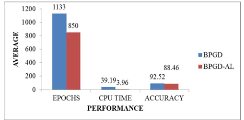
From Table 2, clearly demonstrate that the proposed BPGD-AL algorithm performs well on Card dataset. The proposed BPGD-AL converges to global minima in 3.96 seconds for the CPU Time with the average accuracy of 88.46%. In addition, in term of epochs, BPGD-AL performs very well with 850 epochs as compared to BPGD with 1133 epochs. Figure 1 shows the bar graph of comparison performance between BPGD and the proposed BPGD-AL algorithm for Australian credit card approval dataset.
Fig 1: The comparison performance between BPGD and BPGD-AL algorithm for Australian credit card approval dataset
From the Figure 1, we can see in term of epoch the proposed BPGD-AL algorithm performed the best with 850 epochs as compared to the BPGD algorithm with 1133 epochs. Furthermore, in term of CPU time, the proposed BPGD-AL algorithm also shows the best performance with 3.96 seconds as compared to BPGD algorithm with 39.19 seconds. However, in term of accuracy, BPGD algorithm manages to classify better with the average accuracy of 92.52% as compared to the proposed BPGD-AL algorithm which is 88.46%.
B. Diabetes dataset
The Diabetes dataset is taken from UCI Machine Learning website. The dataset describes that diabetes patient records were obtained from two sources: an automatic electronic recording device and paper records. Therefore, this dataset consists of 384 instances where 193 instances were used for testing. As for the attributes, there are 10 attributes where eight attributes are for input and two attributes are for output. For BPGD algorithm, the best of coefficient momentum is 0.3 and the best of learning rate is 0.3. Whereas for the proposed BPGD-AL algorithm, the best
coefficient momentum is 0.3 and the best of range learning rate is [0.3, 0.4]. Table 3 shows the comparison performance between BPGD and the proposed BPGD-AL algorithm for Diabetes dataset.
TABLEIII
THE COMPARISON PERFORMANCE BETWEEN BPGD AND BPGD-AL ALGORITHM FOR DIABETES DATASET.
BPGD BPGD-AL
Epochs 2664 2595
CPU Time (s) 48.08 26.94
Accuracy (%) 77.91 77.90
SD 2664 2595
Success 30 30
Failure 0 0
In this dataset, BPGD algorithm performs slightly better than the proposed BPGD-AL algorithm in term of the average of accuracy with 77.91%. In term of CPU time, the proposed BPGD-AL outperforms with the average of 26.94 seconds. As for the number of epoch, the proposed BPGD-AL converges to global minima within 2595 epoch rather than BPGD with 2664 epochs. Hence, in this dataset, the proposed BPGD-AL has outperformed BPGD in terms of epochs and CPU time. Figure 2 shows the bar graph of comparison performance between BPGD and the proposed BPGD-AL algorithm for Diabetes dataset.
Fig 2: The comparison performance between BPGD and BPGD-AL algorithm for Diabetes dataset
Figure 2 clearly demonstrate that the proposed BPGD-AL algorithm outperformed BPGD with the best performance in term of epoch and CPU time with 2595 epochs and 26.94 seconds of CPU time as compared to BPGD algorithm with 2664 epoch and 48.08 seconds for CPU time. But, in term of accuracy, BPGD algorithm performs slightly better with the average of 77.91% as compared to the proposed BPGD-AL with average accuracy of 77.90%.
C. Glass dataset
momentum is 0.2 and the best of range learning rate is [0.3, 0.4]. Table 4 shows the comparison performance between BPGD and the proposed BPGD-AL algorithm for Glass dataset.
TABLEIV
THE COMPARISON PERFORMANCE BETWEEN BPGD AND BPGD-AL ALGORITHM FOR GLASS DATASET.
BPGD BPGD-AL
Epochs 2083 2365
CPU Time (s) 44.94 22.31
Accuracy (%) 79.68 77.03
SD 2083 2365
Success 30 30
Failure 0 0
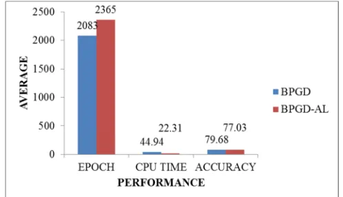
From Table 4, clearly we can see that the proposed BPGD-AL algorithm show a very good performance in term of CPU time with 22.31 seconds as compared to BPGD algorithm which took 44.94 seconds. But in term of epoch and accuracy the BPGD algorithm show the best performance with 2083 epochs and average accuracy is 79.68% as compared with to the proposed BPGD-AL algorithm which took are 2365 epochs and average accuracy is 77.03%. Figure 3 shows the bar graph of comparison performance between BPGD and the proposed BPGD-AL algorithm for Glass dataset.
Fig. 3: The comparison performance between BPGD and BPGD-AL algorithm for Glass dataset
Figure 3 shows the results of simulation for glass dataset on BPGD and the proposed BPGD-AL algorithm. In term of epoch the BPGD algorithm outperforms the proposed BPGD-AL algorithm with 2083 epochs. In term of CPU time, the proposed BPGD-AL algorithm performs the best of average of CPU time with 22.31 seconds as compared to BPGD algorithm which took 44.94 seconds. Hence, in term of accuracy the BPGD algorithm shows the best of average with 79.68% as compared to the proposed BPGD-AL algorithm which took 77.03%. This is probably because the dataset that been used not suit for this simulation and that is why it did not performed very well.
D. Heart dataset
The fourth benchmark problem dataset is heart dataset. The dataset were collected from UCI Machine learning repository which consist of 303 instances, 13 inputs, one output and 75 attributes. This dataset deals with all the symptoms of a heart disease present in a patient on the basis of information given as input. For BPGD algorithm, the best
of coefficient momentum is 0.7 and the best of learning rate is 0.3. Whereas, for the proposed BPGD-AL algorithm, the best coefficient momentum is 0.7 and the best of range learning rate is [0.2, 0.3]. Table 5 shows the comparison performance between BPGD and the proposed BPGD-AL algorithm for Heart dataset.
TABLEV
THE COMPARISON PERFORMANCE BETWEEN BPGD AND BPGD-AL ALGORITHM FOR HEART DATASET.
BPGD BPGD-AL
Epochs 1783 1329
CPU Time (s) 63.58 6.38
Accuracy (%) 90.30 88.46
SD 1783 1329
Success 30 30
Failure 0 0
As demonstrated in the Table 5, the proposed BPGD-AL has it best average CPU time with 6.38 seconds. Moreover, for epochs, BPGD-AL also outperformed where it converges to global minima just within 1329 epochs. In term of accuracy, BPGD is the highest average accuracy with 90.30% as compared to the proposed BPGD-AL. Figure 4 shows that the bar graphs of comparison performance between BPGD and BPGD-AL algorithm for Heart dataset.
Fig 4: The comparison performance between BPGD and BPGD-AL algorithm for Heart dataset
Figure 4 shows that the proposed BPGD-AL performed it best in terms of epoch and CPU time but not very well in term of accuracy. In term epoch, the proposed BPGD-AL algorithm achieved 1329 while BPGD algorithm took 1783. On the other hand, in term of CPU time the proposed BPGD-AL algorithm took only 6.38 seconds while BPGD algorithm need 63.58 seconds to converge. Hence, in term of accuracy, BPGD algorithm shows the best average accuracy with 90.30% and the proposed BPGD-AL algorithm with 88.46%.
E. Horse Colic dataset
performance between BPGD and the proposed BPGD-AL algorithm for Horse Colic dataset.
TABLEVI
THE COMPARISON PERFORMANCE BETWEEN BPGD AND BPGD-AL ALGORITHM FOR HORSE COLIC DATASET.
BPGD BPGD-AL
Epochs 2729 2385
CPU Time (s) 97.90 25.14
Accuracy (%) 80.08 79.09
SD 2729 2385
Success 27 30
Failure 3 0
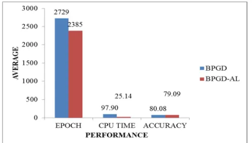
Based on Table 6, it shows that the proposed BPGD-AL algorithm achieved the best in term of epoch as compared to BPGD algorithm with 2385 epochs and CPU time is 25.14 seconds while BPGD took 2729 epochs and 97.90 seconds. But in term of accuracy, the BPGD algorithm still perform better with 80.08% as compared to the proposed BPGD-AL algorithm which took 79.09%. Figure 5 shows that the bar graphs of comparison performance between BPGD and BPGD-AL algorithm for Horse Colic dataset.
Fig 5: The comparison performance between BPGD and BPGD-AL algorithm for Horse Colic dataset
Figure 5 clearly shows that the proposed BPGD-AL algorithm out performed BPGD in term of epoch and CPU time as compared to BPGD algorithm. In term of epoch, the proposed BPGD-AL algorithms need 2385 epochs while BPGD took 2729 epochs. Hence, in term of CPU time, the proposed BPGD-AL algorithms need only 25.14 seconds to converge while BPGD is 97.90. But in term of accuracy, BPGD still performed the best with average accuracy of 80.08% while the proposed BPGD-AL is 79.09%.
IV.CONCLUSION
In this paper, an improved back propagation with adaptive learning rate (BPGD-AL) was proposed to overcome the slow learning of the original BPGD algorithm. The efficiency of the proposed BPGD-AL was investigated by comparing the performance with BPGD algorithm on several classification benchmark datasets taken from the UCI Machinery Learning Repository. The simulation results on
Australian credit card approval demonstrated the
performance of the proposed BPGD-AL algorithm outperforms in terms of number of epochs i.e. 850 and convergence time of 3.96 seconds as compared to BPGD algorithm. For diabetes dataset, the proposed BPGD-AL
algorithm also outperforms in terms of number of epochs i.e. 2595 and a convergence time of 26.94 seconds. Moreover, in glass dataset, the performance of the proposed BPGD-AL algorithm outperforms in terms of convergence with 22.31 seconds when compared with BPGD algorithm. For heart disease dataset, the proposed BPGD-AL algorithm outperforms in terms of 1329 epochs and 6.38 seconds. The above results clearly show that the proposed BPGD-AL
algorithm significantly improved the computational
efficiency of the training process. In the future, this algorithm will be tested against other BP methods especially the hybrid ones and sensitivity analysis on the results will also be performed to find the concreteness in the results.
ACKNOWLEDGMENT
The authors would like to thank Universiti Tun Hussein Onn Malaysia (UTHM) Ministry of Higher Education (MOHE) Malaysia for financially supporting this Research under Trans-disciplinary Research Grant Scheme (TRGS) vote no. T003. This research also supported by GATES IT Solution Sdn. Bhd under its publication scheme.
REFERENCES
[1] Samsudin, N.A., Bradley, A.P. “Group-based meta- classification”. Proceedings - International Conference on Pattern Recognition. Institute of Electrical and Electronics Engineers Inc., 2008.
[2] Samsudin, N.A., Bradley, A.P. “Extended naïve bayes for group based classification”. Advances in Intelligent Systems and Computing. Vol. 287, Springer Berlin Heidelberg, 2014. Page. 497-506.
[3] Rehman, M.Z. and Nawi, N.M. "The effect of adaptive momentum in improving the accuracy of gradient descent back propagation algorithm on classification problems." Communications in Computer and Information Science. Vol. 179 CCIS, Issue. Part I, Springer Berlin Heidelberg, 2011. Page. 380-390.
[4] Waddah Waheeb, Rozaida Ghazali. “Chaotic Time Series Forecasting Using Higher Order Neural Networks”. International Journal on Advanced Science, Engineering and Information Technology, Vol. 6 (2016) No. 5, pages: 624-629.
[5] Jabril Ramdan, Khairuldin Omar, Mohammad Faidzul, “A Novel Method to Detect Segmentation points of Arabic Words using Peaks and Neural Network”. International Journal on Advanced Science, Engineering and Information Technology, Vol. 7 (2017) No. 2, pages: 625-631
[6] Nazri Mohd Nawi, Muhammad Zubair Rehman, and Abdullah Khan. "A New Bat Based Back-Propagation (BAT-BP) Algorithm." Advances in Systems Science. Springer International Publishing, 2014. 395-404.
[7] Senan, N., Ibrahim, R., Nawi, N.M., Mokji, M.M. “Feature extraction for traditional Malay musical instruments classification system”, SoCPaR 2009 - Soft Computing and Pattern Recognition, 2009. Page. 454-459.
[8] Siti Mariyam Shamsuddin, Ashraf Osman Ibrahim, and Citra Ramadhena. Weight Changes for Learning Mechanisms in Two-Term Back-Propagation Network. INTECH Open Access Publisher, 2013.
[9] He Qin. "Neural Network and its Application in IR." Graduate School of Library and Information Science, University of Illinois at Urbana-Champaign Spring (1999).
[10] Chiroma, H., Abdul-Kareem, S., Khan, A., Nawi, N.M., Ya'U Gital, A., Shuib, L., AbuBakar, A.I., Rahman, M.Z., Herawan, T. “Global warming: Predicting OPEC carbon dioxide emissions from petroleum consumption using neural network and hybrid cuckoo search algorithm”, Vol. 10, Issue. 8, PLoS ONE, 2015, page. 548-552. [11] Magoulas, George D., Michael N. Vrahatis, and George S.
[12] Dao, Vu NP, and V. R. Vemuri. "A performance comparison of different back propagation neural networks methods in computer network intrusion detection." Differential equations and dynamical systems 10.1&2 (2002): 201-214.
[13] N. A. Hamid, N. M. Nawi and R. Ghazali, “The Effect of Adaptive Gain and Adaptive Momentum in Improving Training Time of Gradient Descent Back Propagation Algorithm on Classification Problems,” Proceeding of the International Conference on Advanced Science, Engineering and Information Technology 2011. Putrajaya, Malaysia.
[14] Norhamreeza Abdul Hamid, et al. "Accelerating Learning Performance of Back Propagation Algorithm by Using Adaptive Gain Together with Adaptive Momentum and Adaptive Learning Rate on Classification Problems."Ubiquitous Computing and Multimedia Applications. Springer Berlin Heidelberg, 2011. 559-570. [15] Norhamreeza Abdul Hamid, et al. "Learning Efficiency Improvement
of Back Propagation Algorithm by Adaptively Changing Gain Parameter together with Momentum and Learning Rate." Software Engineering and Computer Systems. Springer Berlin Heidelberg, 2011. 812-824.
[16] Norhamreeza Abdul Hamid, et al. "Solving Local Minima Problem in Back Propagation Algorithm Using Adaptive Gain, Adaptive Momentum and Adaptive Learning Rate on Classification Problems." International Journal of Modern Physics: Conference Series. Vol. 9. World Scientific Publishing Company, 2012
[17] Kröse, Ben, et al. "An introduction to neural networks." (1993). [18] Chien Cheng Yu,and Bin Da Liu,”A backpropogation algorithm with
adaptive learning rate and momentum coefficient,” IEEE,2002 [19] Shao, H., and Zheng, H.,” A new bp algorithm with adaptive
momentum for FNNs training,” in: GCIS 2009, Xiamen, China, pp. 16--20 (2009)
[20] Magoulas, G. D., Plagianakos, V. P., & Vrahatis, M. N. (2000, July). Development and convergence analysis of training algorithms with local learning rate adaptation. In Neural Networks, IEEE-INNS-ENNS International Joint Conference on (Vol. 1, pp. 1021-1021). IEEE Computer Society.
[21] Magoulas, G. A., Plagianakos, V. P., & Vrahatis, M. N. (2002). Globally convergent algorithms with local learning rates. Neural Networks, IEEE Transactions on, 13(3), 774-779.