Vol.8 (2018) No. 1
ISSN: 2088-5334
Comparative Study of Density over Time by Several Approaches
Using Individual and Sample Data in the Mixed Traffic
Fadly Arirja Gani
#, Toshio Yoshii
*, Shinya Kurauchi
* #Graduate School of Science and Engineering, Ehime University, 3, Bunkyo-cho, Matsuyama, 790-8577, Japan E-mail: [email protected]
*
Department of Civil and Environmental Engineering, Ehime University, 3, Bunkyo-cho, Matsuyama, 790-8577, Japan E-mail: [email protected]; [email protected]
Abstract— At the macroscopic perspective, traffic analysis requires the knowledge of Fundamental Diagram, which involves the relationship between the variables of density, flow, and speed. As one of the macroscopic traffic flow variables, density can be derived by several approaches. At first, the density of traffic was measured over space, which difficult to be collected mainly in the long section of the road. Therefore, the density variable was simply derived from the fundamental relation of macroscopic traffic flow variable. By this method, the individual speed and flow variable are required in the local measurement. Both traffic density and flow will apply the concept of PCU, which refers to the Indonesian Highway Capacity Manual, 1997 to consider the different characteristic of the vehicle. In the mixed traffic of developing countries, providing traffic data was difficult due to the limitation of the traffic sensor infrastructures. Frequently, providing density variable relies on the sample data for speed analysis. In the present study, the estimation of density will focus on the local measurement over a time interval. By using individual data, density is proposed to be measured directly over time, in which the equation can be modified to utilize the sample data. The number of sample for speed analysis will be varied to know the accuracy and the performance of each approach in the density estimation of mixed traffic. Several approaches for density estimation will be summarized and compared each other. Theoretically, the estimated density which measured over time and space by using individual data can provide the most appropriate result. So, this estimated density will be established as an actual density throughout the study. Then, the performance of each approach either using individual or sample data will be evaluated upon the actual traffic density by mean absolute percentage error (MAPE). The result shows by using the same trap length to measure the speed, the existing and the proposed approaches provide a good estimation of density either by utilizing individual data or sample data of the vehicle speed. This result was indicated by the MAPE value, which obtained under ten percent. Based on the further evaluation of the MAPE value, the performance of each approach was changed by utilizing the different category of data. In addition, estimation of traffic density which utilizes the sample data of vehicle speed has good reliability.
Keywords— density; mixed traffic; passenger car unit; local measurement; time interval
I. INTRODUCTION
Transportation has a major role in the economic growth of a country. In Asian developing countries, the high growth targets to be achieved by government causes the demand for transportation was increasing rapidly. The increasing of transportation demand led to the traffic congestion and safety. In the urban area, the space for the infrastructures was limited while the automobile was growing faster. So, this condition requires the ability to optimize the utilization of the current infrastructure by managing the traffic itself. Essentially, planning, design, and operation of the transportation system require the knowledge of fundamental traffic flow characteristic: flow, density, and speed. These three variables were known as the macroscopic traffic flow variable. These variables were necessary to be acquired for
analyzing the traffic at the macroscopic perspective. Taking the measurement of macroscopic traffic flow variables can be distinguished based on the concept and the measurement interval [1]. The concept was varied according to the response to the characteristic of vehicles in the traffic analysis, such length of the vehicle and projected area of the vehicle [2]–[5]. And, the measurement interval was classified into three: time, space, and time-space interval.
any time instant. By the existence of sensor infrastructure in developed countries, taking the measurement of density over space was considered more difficult. Due to the difficulties, providing the density variable was developed by a different approach, where each approach will lead to the different estimated density value. The most convenient approach is derived density from the fundamental relation of macroscopic traffic flow variable. The estimated density by each approach may deviate from the actual density.
Briefly, this study focuses on investigating the approaches to derive the proper density in the mixed traffic by using sample data in the local measurement. So, the density will be estimated by a different approach. Basically, it was not known yet clearly which kind of approach can represent the actual traffic density in the most appropriate. Defining the approach for estimating the actual density was required to be established as the reference to assess the performance of the other approaches. Theoretically, a density which measured over time and space interval can provide the best-estimated value to represent the actual traffic density variable. This approach utilizes the individual data. Then, the effect of different approach can be shown by comparing each estimated density either utilize the individual or the sample data of vehicle speed. The analysis result will show which kind of approaches can provide a small error as compared to actual density. Finally, the proper approach to estimate the density variable in the mixed traffic can be obtained.
II. MATERIAL AND METHOD
In the present study, two approaches are proposed to estimate the actual traffic density over time for utilizing the sample data. Then, several existing and the proposed approaches will be compared to estimate the actual traffic density variable based on the field observation data.
A. Field Data
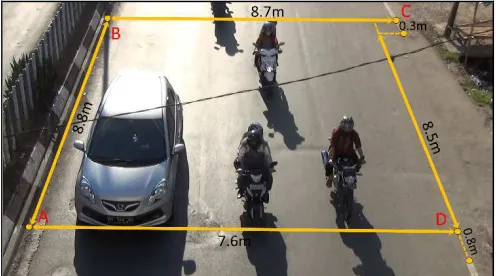
In this study, field data were collected at a mid-block section of two-lane urban road with a width of 8.7 meters in Makassar, Indonesia. Since the Indonesian highway was not equipped with the sensor infrastructure, the traffic data will be collected manually by video recording. The traffic condition of Urip Sumoharjo Street was observed through video camera from the pedestrian bridge on 20th September 2013 at 08.30-11.30 a.m. in sunny conditions. The observation of traffic considers a short section of a road as the detection zone with 8.8 meters in longitudinal length as seen in Fig. 1.
Fig. 1 Detection zone of the observation area
The video data will be converted into image data for 10 frames per second, then the arrival time and departure time for each vehicle will be recorded. The individual data will be shown for every minute. All the motorized vehicle in the share of traffic will be classified into three categories: motorcycle (mc), passenger car/light vehicle (lv), and heavy vehicle (hv).
B. Macroscopic Traffic Flow Variables
At the macroscopic perspective, three main variables: density k, flow rate q, and mean speed u are always connected by the identity relation of Fundamental Diagram in the Equation (1).
u
k
q
=
⋅
(1) This fundamental relation shows that knowing two variables automatically leads to the third. There are three different ways to represent the relationship between the macroscopic variables in the two-dimensional diagram:q=Q(k), u=U(k), and u=U(q). Generally, these three
relations were plotted to show the capacity flow and describe the condition of traffic, where the relation q=Q(k) between flow and density was the most often used. Simply, in single regime model, traffic was distinguished into two: uncongested phase and congested phase, which separated vertically at the critical density kc in the x-axis. The point of critical density kc in the x-axis will provide the capacity flow in the y-axis. In share of the road, the characteristic of traffic either at microscopic or macroscopic perspective was influenced by all surrounding stationary and moving objects (vehicles, median, and roadside activities). In addition, the adverse weather like rainfall in most developing countries also affects the microscopic and macroscopic traffic flow variables such as headway, density, flow and speed [6], [7]. The effect of the adverse weather in the traffic characteristic confirmed that this factor induced the reduction of road capacity [8].
Basically, it was widely known that the traffic flow q was measured directly over time and density k was measured over space by the Equation (2) and Equation (3) respectively.
T
n
q
∆
=
(2)X
m
k
∆
=
(3)where n - the number of the vehicle that passes a cross-section of the road during a time interval ∆T; m - the number
of the vehicle across a road section with ∆X length at an
instantaneous time.
∈
=
→
=
s i
i s
i
i
v
n
u
v
n
u
1
1
(4)
m
v
u
=
i i (5) where vi - the speed of vehicle i; ns - the number of vehicle sample that passes a cross-section of the road during a time interval ∆T.At the macroscopic perspective, density variable was often used to describe and model the actual traffic state with the flow variable. Density is a traffic measure which explains the extent of usage of road space by vehicles. Density is the other term of concentration which used interchangeably as one of the macroscopic traffic flow variables. Traffic density can be derived by several approaches. In the earlier study, a comparative evaluation of density estimation method in India has been conducted [9], [10]. The study compares several methods to derive density by assuming the traffic under a homogeneous condition in the vehicle unit. So, the different characteristic of the vehicle was not considered yet in the comparison. The estimated density over space was established to represent the actual density, which used to assess the performance of the other estimation method. In the measurement of space, density was defined as the number of vehicles observed for a specified length of road at a given time instance. At first, density considers neither the length nor the width of the vehicle. If similar types of vehicles are traveling on the road, density gives a fairly accurate measure of traffic quality. Density, expressed as a number of vehicles per unit length of roadway, is valid only under highly homogeneous traffic conditions, wherein the difference in individual vehicle speeds and vehicle dimensions are negligible. In practice, however, even under homogeneous traffic conditions, there are significant differences in the term two characteristics (speed and dimension) of vehicles. Therefore, it is important to consider the characteristic of the vehicle in the traffic analysis. The passenger car unit or PCU is one of the concepts, which has proposed to incorporate the characteristic of the vehicle in the traffic analysis. This concept was also known as passenger car equivalent (PCE), which first specifically addressed significantly in Highway Capacity Manual 1965 [11] to distinguish the characteristic of truck and passenger car.
In order to consider the characteristic of vehicles in the traffic analysis, the concept of PCU will be adopted to define the macroscopic traffic flow variable. By adopting the concept of passenger car unit, density k over space can be expressed by the Equation (6).
(
)
X
m
k
j j j∆
⋅
=
α
(6)where m, mj - the number of vehicle/vehicle category j across a road section with ∆X length at the instantaneous
time; αj - passenger car equivalent of a vehicle category j. Since, taking the measurement over space is difficult, providing density are developed to be derived from the other approach. Theoretically, density variable can be obtained by the other measurement interval: time interval and time-space interval. Taking the measurement of macroscopic traffic
flow variable at three different intervals can provide a similar result under homogeneous and stationary condition. In the local measurement with a time interval ∆T at the
specific point, density variable can be directly observed. In the reality condition, the measurement over space interval and time interval may differ each other. The relation between both intervals has been investigated by the earlier study which analyzes the relating time-occupancy measurement and space-occupancy measurement [12]. It shows that the location of time-occupancy measurement along the section of road has an influence on the resulting estimation bias.
By understanding the concept of measurements interval of macroscopic traffic flow variable, density in PCU over space in Equation (6) can be expanded into the time-space interval [13], [14]. In the measurement over time and space, the definition of density in PCU can be expressed in the Equation (7).
( )
(
)
X
T
t
k
j j i j i∆
⋅
∆
⋅
=
α
∈ (7)where ti - occupied time or time spent by the vehicle i on the measurement interval ∆T and ∆X.
In the other measurement interval, the definition of density in PCU which measured over time and space as seen in the Equation (7) can be transformed to obtain density over time [1]. It can be expressed in the Equation (8).
T
v
k
j i j ij
∆
⋅
=
∈1
α
(8)
In the other approach, density can be derived by using the identity relation of Fundamental Diagram as shown in the Equation (9).
u
q
k
=
(9)Basically, the Equation (9) was developed in homogeneous traffic [15], [16], even though it still valid for the mixed traffic condition [17]. In this approach, density k can be derived by defining the flow q and speed u in advance. Basically, the flow variable q is measured directly over time which has widely known as seen in the Equation (2). By adopting the concept of passenger car unit, the flow can be modified as seen in the Equation (10).
(
)
T
n
q
j j j∆
⋅
=
α
(10)where, n, nj - the number of vehicle/vehicle category j that passes a cross-section of the road during a time interval ∆T;
αj - passenger car equivalent of a vehicle category j.
T
v
k
i i∆
=
1
(11)
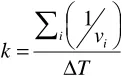
Since, the PCU concept was adopted to estimate density variable, defining the speed u may be different. Some argue that by using sample data, the weighted average individual speed as seen in the Equation (12) was more appropriate than space mean speed [18].
( )
( )
js( )
s ji i
j j j j j j
n
v
v
n
v
n
u
, ,
;
∈=
⋅
=
(12)where
v
j - the average speed of vehicle category j; nj,s -number of sample of vehicle category j that passes a cross-section of road per time unit.
In case using individual data, nj,s will be equal to the nj. So, the definition of mean speed in the Equation (12) will be equal to the normal arithmetical average individual speed in the time interval or also known as time mean speed as seen in the Equation (13).
( )
(
)
( )
n
( )
v
u
n
v
u
i ij j
j i j i
=
↔
=
∈ (13)The term of time mean speed in the Equation (13) and the mean speed in the Equation (5) are different. The mean speed in the Equation (5) is derived from the instantaneous measurement in space interval, and time mean speed is derived by the local measurement in the time interval. So, in a homogeneous condition, acquiring the density by using the time mean speed in the Equation (13) does not satisfy the identity relation of Fundamental Diagram.
C. Traffic Density Estimation
As one of the macroscopic variables, density variable is used to describe and estimate the actual traffic state. So, it makes providing the proper density variable was getting necessary to obtain the appropriate model for estimating the actual traffic state. In the present study, the new approach is proposed to determine density in the mixed traffic condition. The performance of several approaches for density estimation will be summarized and evaluated. A case study of traffic in Makassar, Indonesia will be conducted for this comparative study. The individual data were required for the analysis, where it will be utilized to derive the macroscopic traffic flow variable: density, flow, and speed for every minute. In the analysis or study of mixed traffic, the characteristic of the vehicle was getting more important to be considered due to the large variation in the share of the road. In order to consider the characteristic of the vehicles in the traffic analysis at macroscopic perspective, the concept of Passenger Car Unit or PCU will be adopted to express the traffic density and flow variable. In the present study, the concept of passenger car unit refers to the Indonesian Highway Capacity Manual, 1997, which the motorized vehicle in the share of traffic will be classified in three categories: motorcycle, passenger car or light vehicle and heavy vehicle [19]. Converting all vehicles into passenger car will adopt PCU value as shown in Table 1.
TABLEI
PASSENGER CAR EQUIVALENT VALUE
Type of Vehicle PCE-Value
Motorcycle (MC) 0.4
Light Vehicle (LV) 1
Heavy Vehicle (HV) 1.3
In the mixed condition, estimating traffic density in PCU by using individual data can provide a better description of the actual condition of traffic density. Since the characteristic of mixed traffic does not follow the lane rule, density will be estimated per direction of the road. The Approach 1 that will be adopted to estimate the density is measured directly over time and space as illustrated in Fig. 2.
Fig. 2 Traffic density over time and space
In Fig. 2, the actual traffic density will be estimated in the measurement area which shown by the shaded area of the two-dimensional diagram. In the measurement area over a time interval ∆T and space interval ∆X, density in PCU can
be defined by the Equation (7) in the previous section. According to the illustration in the Fig. 2, the time spent by vehicle i on the measurement interval ∆T and ∆X, (ti) can be expressed by the Equation (14).
(
t
T
)
(
t
(
T
T
)
)
t
i=
min
i,2,
−
max
i,1,
−
∆
(14) Where, ti,1, ti,2 - the arrival and departure time of vehicle i in the detection zone.In the Equation (14), the arrival and departure time show the time when the trajectory line of vehicle i get the entry point and the exit point of the detection zone respectively. The Approach 1 can be adopted by substituting the Equation (14) into the Equation (8), which requires the individual data for traffic density estimation. By utilizing the individual data in the time-space interval, the Approach 1 can provide the most appropriate estimation of the actual traffic density.
Taking the measurement of traffic density, which involves the space interval ∆X is difficult, especially for the long
section of road. Due to the difficulties of the measurement, density over a time interval ∆T become an alternative to be
(9). By adopting the Equation (9), two other approaches for density estimation can be derived by a different definition of speed. The Approach 2 and 3 adopt the space mean speed as the Equation (4) and the weighted average individual speed as the Equation (12) respectively. The Approach 2 and 3 can be expressed by the Equation (15) and Equation (16), where both equations can utilize the individual and sample data.
(
)
s s i
i j j j
n
v
T
n
k
∈
⋅
∆
⋅
=
1
α
(15)(
)
( )
( )
⋅
⋅
∆
⋅
=
∈ j s j s j i i j j jj j j
n
v
n
n
T
n
k
, ,α
(16)As mention earlier, traffic density k also can be directly measured over time by the Equation (8). So, in the Approach 4, the Equation (8) will be adopted to estimate density over time, however this equation only suitable for utilizing the individual data. Since providing the individual data was difficult, utilizing the sample data is another option to provide density variable. Therefore, in the present study, the Equation (8) is proposed to be modified for utilizing the sample data by the Equation (17).
T
v
n
k
j j j j∆
⋅
=
α
(17)where
v
j - the mean speed of vehicle category j.In the Equation (17), two approaches for density estimation can be derived by defining the mean speed of vehicle category j differently. The mean speed can be represented by the normal arithmetical average of individual speed as the Equation (18) and the harmonic mean speed as the Equation (19).
( )
∈⋅
=
i js i s j jv
n
v
, ,1
(18)
∈
=
s j i i s j jv
n
v
, ,1
(19)By substituting the Equation (18) and the Equation (19) into the Equation (17), the Approach 5 and 6 can be formulated as the Equation (20) and the Equation (21) respectively.
( )
T
v
n
n
k
j s j i i s j j j∆
⋅
⋅
=
∈, ,α
(20)T
v
n
n
k
j i js i
s j j j
∆
⋅
⋅
⋅
=
∈, ,1
1
α
(21)In case using individual data, nj,s will be equal to the nj. It makes the Equation (21) will be equal to the Equation (8). Therefore, estimating the traffic density by the Approach 6 and 4 using individual data will produce a similar result.
Briefly, in this study, density variable will be estimated by six different approaches, which summarized in Table 2.
The basic concept for traffic density estimation which adopted each approach in Table 2 can be explained as the following:
• Approach 1: traffic density will be estimated by taking the measurement directly over a time interval ∆T and
space interval ∆X.
• Approach 2: traffic density was derived from the identity relation of Fundamental Diagram by using the harmonic mean speed.
• Approach 3: traffic density was derived from the identity relation of Fundamental Diagram by using the weighted average individual speed.
• Approach 4: traffic density will be estimated by taking the measurement directly over a time interval ∆T. • Approach 5: the concept was derived by modifying
the Approach 4, where the normal arithmetical average will be adopted to utilize the sample data of vehicle speed.
• Approach 6: the concept was derived by modifying the Approach 4, where the harmonic mean will be adopted to utilize the sample data of vehicle speed.
TABLEII
APPROACH FOR DENSITY ESTIMATION
The approach for density estimation
Approach 1
(
( )
)
X
T
t
k
j j i j i∆
⋅
∆
⋅
=
α
∈Approach 2
(
)
s s
i i
j j j
n
v
T
n
k
∈
⋅
∆
⋅
=
1
α
Approach 3(
)
( )
( )
⋅
⋅
∆
⋅
=
∈ j s j s j i i j j jj j j
n
v
n
n
T
n
k
, ,α
Approach 4T
v
k
j i j ij
∆
⋅
=
∈1
α
Approach 5
( )
T
v
n
n
k
j s j i i s j j j∆
⋅
⋅
=
∈, ,α
Approach 6T
v
n
n
k
j i js
i s j j j
∆
⋅
⋅
⋅
=
∈, ,1
1
α
sample for each vehicle type was varied to know the performance and the limitation of the approach to estimate density by utilizing the sample data. There will be 10 categories of sample data, which will be utilized in the present study as seen in Table 3.
TABLEIII
VARIATION OF NUMBER OF SAMPLE DATA
Type of data Number of samples
MC LV HV
Sample data 1 (SD1) 5 2 2
Sample data 2 (SD2) 5 3 2
Sample data 3 (SD3) 5 5 2
Sample data 4 (SD4) 5 7 2
Sample data 5 (SD5) 5 9 2
Sample data 6 (SD6) 10 5 2
Sample data 7 (SD7) 15 5 2
Sample data 8 (SD8) 20 5 2
Sample data 9 (SD9) 7 7 2
Sample data 10 (SD10) 9 9 2
In Table 3, the sample of a heavy vehicle will not be varied like two others vehicle. Since the share of the heavy vehicle was not significant, the number of samples were established equal to the number of the vehicle for each time interval and no more than two vehicles. The number of the sample may change between one and two vehicles and fixed for all categories of sample data. Therefore, the effect of a heavy vehicle will not be much discussed throughout the study. By using several approaches in Table 2 to utilize the different categories of data in Table 3, there will be 44 different values of estimated density. All the combination of the traffic density estimation can be seen in Table 4.
TABLEIV
COMBINATION OF ESTIMATED DENSITY
The approach for
density estimation Type of data
Approach 1 ID
Approach 2 ID, SD1, SD2, SD3, SD4, SD5, SD6,
SD7, SD8, SD9, SD10
Approach 3 ID, SD1, SD2, SD3, SD4, SD5, SD6,
SD7, SD8, SD9, SD10
Approach 4 ID
Approach 5 SD1, SD2, SD3, SD4, SD5, SD6,
SD7, SD8, SD9, SD10
Approach 6 SD1, SD2, SD3, SD4, SD5, SD6,
SD7, SD8, SD9, SD10
The effect of sample data on the performance of each approach will be evaluated. All the estimation value of density by different approaches will be compared. In the comparison, the density value which measured over time and space by using individual data will be considered as an actual value. Then, the error of density value by the other approaches can be shown by the statistic measurements: Mean Absolute Percentage Error (MAPE), which expressed by the Equation (22).
=−
⋅
=
Ni
i actual
i estimated i
actual
x
x
x
N
MAPE
1
, , ,
1
(22)where xactual,i - the estimated density by the Approach 1, which utilize the individual data at period i; xestimated,i - the estimated density by the others combination at period i.
III.RESULTS AND DISCUSSION
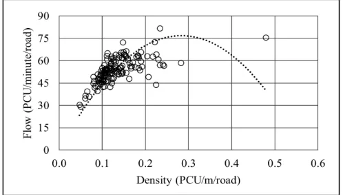
In the present study, the observed data were analyzed to derive the traffic density by several approaches for every minute. By the one-minute interval, there are 148 observed data, which have been collected during three-hour observation. The remaining data were not used due to the error at the collecting stage. Briefly, the condition of traffic during the observation period can be described by plotting the density and flow variable in the two-dimensional diagram in Fig. 3.
Fig. 3 Density-flow plane
In Fig. 3, the traffic flow was measured over time, and density was estimated by the Approach 1, where both variables are presented in passenger car unit for every minute. The Fig. 3 shows simply that the condition of traffic data during the observation period was mostly in the uncongested phase. In addition, the composition of traffic during the observation period is shown in Fig. 4 and Fig. 5.
Fig. 4 Traffic composition
Fig. 5 Proportion of vehicle for each category
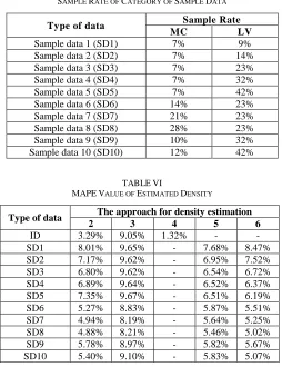
Table 5 provides the additional information about the sample number of motorcycle and passenger car, which established in the present study. The sample rate in Table 5 will not be much discussed throughout the study, but it still useful to provide a simple description of how big the sample as compared to the real traffic. According to the Table 4, several estimated values of traffic density will be obtained by the different approach and category data. Then, all the estimated density is evaluated and compared each other. As mention earlier, the traffic density which estimated by using the Approach 1 will be compared to the other approaches to provide: mean absolute percentage error (MAPE). The MAPE value for all estimated density in different approach and type of data can be seen in Table 6.
TABLEV
SAMPLE RATE OF CATEGORY OF SAMPLE DATA
Type of data Sample Rate
MC LV
Sample data 1 (SD1) 7% 9%
Sample data 2 (SD2) 7% 14%
Sample data 3 (SD3) 7% 23%
Sample data 4 (SD4) 7% 32%
Sample data 5 (SD5) 7% 42%
Sample data 6 (SD6) 14% 23%
Sample data 7 (SD7) 21% 23%
Sample data 8 (SD8) 28% 23%
Sample data 9 (SD9) 10% 32%
Sample data 10 (SD10) 12% 42%
TABLEVI
MAPEVALUE OF ESTIMATED DENSITY
Type of data The approach for density estimation
2 3 4 5 6
ID 3.29% 9.05% 1.32% - -
SD1 8.01% 9.65% - 7.68% 8.47%
SD2 7.17% 9.62% - 6.95% 7.52%
SD3 6.80% 9.62% - 6.54% 6.72%
SD4 6.89% 9.64% - 6.52% 6.37%
SD5 7.35% 9.67% - 6.51% 6.19%
SD6 5.27% 8.83% - 5.87% 5.51%
SD7 4.94% 8.19% - 5.64% 5.25%
SD8 4.88% 8.21% - 5.46% 5.02%
SD9 5.78% 8.97% - 5.82% 5.67%
SD10 5.40% 9.10% - 5.83% 5.07%
The statistic indicator in Table 6 will be used to evaluate the performance of each approach either using individual data or several variations of sample data of vehicle speed. The result shows the variation of the performance of each approach by the change MAPE value for all categories of data. Generally, all the approaches which used to derive the traffic density have a good performance. It was indicated by the MAPE value, which obtained under 10% as compared to estimated density over time and space interval. The evaluation of all estimated density can be more understandable by plotting the MAPE value into the chart which clustered over the approach and type of data as seen in Fig. 6.
Fig. 6 MAPE value of estimated density
In Fig. 6, the analysis result shows that the Approach 3 has the lowest performance, which indicated by the highest error for all the variation of the type of data. Naturally, it shows clearly the more sample data, the better of the result of traffic density estimation. It was indicated by the trend of MAPE value of each approach decreased between SD1 and SD8, where the number of samples was increased.
Fundamental Diagram. Therefore, the estimated density by the Approach 3 will be higher than any other approach.
For more detail analysis, the performance of each approach to utilizing the individual data and sample data will be evaluated separately. The MAPE value of each density, which estimated by several approaches to utilize the individual data can be seen in Fig. 7.
Fig. 7 Estimated density using individual data
In Fig. 7, the result shows that the Approach 4 can estimate traffic density over time very well with lowest MAPE value: 1.32% as compared to the Approach 2 and Approach 4 by 3.29% and 9.05%. And, for utilizing the variation of sample data, the performance of several approaches will be evaluated separately by different type of sample data. At first, the approaches will be evaluated in the category of sample data SD1, SD2, SD3, SD4, and SD5. In these three categories, the number of sample of the motorcycle was fixed with 5 vehicles and sample for the passenger car will be varied by 2, 3, 5, 7, and 9 vehicles. By utilizing these categories of sample data, the MAPE value for all approaches can be seen in Fig. 8.
SD1: mc (5), lv (2), and hv (2); SD2: mc (5), lv (3), and hv (2); SD3: mc (5), lv (5), and hv (2); SD4: mc (5), lv (7), and hv (2); SD5: mc (5), lv (9), and hv (2)
Fig. 8 Estimated density using sample data 1, 2, 3, 4, and 5
In Fig. 8, the result shows that both Approach 5 and 6 provides a good performance, where the trend of MAPE value was decreased by the increasing number of sample for a passenger car. In the first three categories of sample data: SD1, SD2, and SD3, the Approach 5 has a better performance than the others, which indicated by the lowest MAPE value. And the remaining categories: SD4, and SD5,
the Approach 6 has better performance for density estimation. Moreover, the trend was different for the Approach 2 and 3. In the Approach 2, the trend was changed in the category of SD4 and SD5. In both categories of SD4 and SD5, the number of sample for passenger car was more than the motorcycle, in which the individual data shows the opposite in the earlier discussion about traffic composition. This case illustrates the limitation of the Approach 2 for density estimation, where the number of sample for each vehicle category should notice the composition of traffic. And for the Approach 3, the increasing of the sample for passenger car does not provide a significant difference in the MAPE value.
Furthermore, the MAPE values of the Approach 5 and 6 in the data categories of SD4, and SD5 did not change significantly as compared to previous category SD3. So, it means, taking 5 samples for a passenger car as used in category SD3 is quite enough to represent the overall speed of this vehicle type. This specific number was affected by the average of individual data for the passenger car.
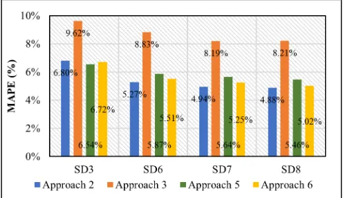
In the further evaluation, the performance of several approaches will be compared in the category of sample data: SD3, SD6, SD7, and SD8. In these categories, it will consider more sample of the motorcycle. The number of sample for the motorcycle will be varied by 5, 10, 15, and 20 vehicles and sample for the passenger car was fixed with 5 vehicles. The MAPE value for all approaches can be seen in Fig. 9.
SD3: mc (5), lv (5), and hv (2); SD6: mc (10), lv (5), and hv (2); SD7: mc (15), lv (5), and hv (2); SD8: mc (20), lv (5), and hv (2) Fig. 9 Estimated density using sample data 3, 6, 7, and 8
In addition, the Fig. 9 shows that the MAPE values of the Approach 2, 5 and 6 in the data categories of SD7 and SD8 did not change significantly as compared to previous categories SD6. So, it means, taking 10 samples for the motorcycle as used in category SD6 is quite enough to represent the overall speed of this vehicle category. The representative number of sample was dependent on the average of individual data for the motorcycle.
In the last evaluation, the performance of several approaches will be compared in the category of sample data: SD3, SD9, and SD10. In these categories, the number of sample of motorcycle and passenger car will be set equal to 5, 7, and 9 vehicles. The MAPE value for each approach can be seen in Fig. 10.
SD3: mc (5), lv (5), and hv (2); SD9: mc (7), lv (7), and hv (2); SD10: mc (9), lv (9), and hv (2)
Fig. 10 Estimated density using sample data 3, 9, and 10
In Fig. 10, the result shows that when the number of sample for motorcycle and passenger car is equal, the Approach 6 provides better performance than the other approaches. The category of SD3 is an exception, where the Approach 5 gives the lowest MAPE value. This case confirmed the previous evaluation in Fig. 8. So, it can be interpreted that in the relatively small sample, the Approach 5 was better than the other, even the sample for motorcycle and passenger car is equal. In Fig. 10, the MAPE value of the approach 5 between the category of SD9 and SD10 slightly increased, where it should be decreased by the increasing number of sample. The result informs that the same number of sample of motorcycle and passenger car may affect the performance of the Approach 5 as shown in category SD10, which has a relatively larger number of sample.
IV.CONCLUSION
This study evaluates several approaches to derive the density variables with passenger car unit in the mixed traffic condition. The result of this study shows that generally, all the approach provides a good performance by the MAPE value under 10 % on the same trap length for measuring the speed of the vehicle. In more specific, the performance of each approach can be examined based on the variation of the category of data. By utilizing the individual data, the Approach 4 has the highest performance to estimate the density variable. And for utilizing the sample data, the performance of each approach was examined separately in
several categories. The performance of each approach varied by different category of sample data. The Approach 5 shows highest performance in the category of data: SD1, SD2, and SD3, which has a relatively small number of sample. In the sample data SD4, SD5, SD9, and SD10, the Approach 6 provides better performance than the others. And, the Approach 2 was better in the sample data SD6, SD7, and SD8. Based on the evaluation, the composition of the vehicle sample affected the performance of Approach 2. Therefore, determining the number of sample for each vehicle category in the Approach 2 should consider the actual share of traffic. There are several cases, which make the composition of vehicle sample cannot match with the actual share of traffic such as no initial information about the actual composition of traffic, and the number of the sample is given or obtained by the other observed data: Probe and Bluetooth data. So, in these cases, the other approaches are required to solve the limitation of the Approach 2. In the present study, the Approach 5 and 6 are proposed to estimate the density by utilizing the sample data. Both the Approach 5 and 6 produce a better estimation of traffic density, which indicated by the change trend of MAPE value to utilize the different sample data.
Moreover, the accuracy of the estimation of traffic density by utilizing the category of sample data was also acquired. It shows that the estimation of the traffic density over time for all approaches provides an error that not much different with the individual data. Therefore, by the limitation of resources to provide the traffic data, the estimation of density variable by utilizing the sample data of vehicle speed was reliable.
ACKNOWLEDGMENT
The authors would like to acknowledge the financial support through the scholarship given by Directorate General of Higher Education of Indonesia.
REFERENCES
[1] Gani FA, Yoshii T, Kurauchi S. The Suitable Index of Flow and Density in the Mixed Traffic. IOP Conf Ser Earth Environ Sci [Internet]. 2017 Jun [cited 2017 Jun 23];71(1):12015. Available from:
http://stacks.iop.org/1755-1315/71/i=1/a=012015?key=crossref.0626bbb7f39fd01816a857fa329 94145
[2] Chari SR, Badarinath KM. Study of mixed traffic stream parameters through time lapse photography. Highw Res Bull (Indian Road Congr Highw Res Board) [Internet]. 1983 [cited 2016 Nov 25];20:57–83.
Available from:
http://www.safetylit.org/citations/index.php?fuseaction=citations.vie wdetails&citationIds%5B%5D=citjournalarticle_486942_38 [3] Mallikarjuna C, Rao KR. Area occupancy characteristics of
heterogeneous traffic. Transportmetrica [Internet]. 2006 [cited 2015 Aug 27];2(3):223–36. Available from: http://www.tandfonline.com/doi/abs/10.1080/18128600608685661 [4] Arasan VT, Dhivya G. Methodology for Determination of
Concentration of Hetrogeneous Traffic. J Transp Syst Eng Inf Technol [Internet]. 2010;10(4):50–61. Available from: http://dx.doi.org/10.1016/S1570-6672(09)60052-0
[5] Gani FA, Yoshii T, Kurauchi S. The Effect of Heterogeneity of Vehicle Size on the Fundamental Diagram in Mixed Traffic. (Case Study: Makassar Traffic on Urip Sumoharjo Street). In: Proceeding of the International Conference of Transdiciplinary Research on Environmental Problem in Southeastern Asia. Makassar, Indonesia: Penerbit ITB; 2014. p. 95–104.
Available from: http://ijaseit.insightsociety.org/index.php?option=com_content&view =article&id=9&Itemid=1&article_id=177
[7] Alhassan HM, Ben-Edigbe J. Effect of Rain on Probability Distributions Fitted to Vehicle Time Headways. Int J Adv Sci Eng Inf Technol [Internet]. 2012 [cited 2017 Jul 23];2(2):144–50.
Available from:
http://ijaseit.insightsociety.org/index.php?option=com_content&view =article&id=9&Itemid=1&article_id=173
[8] Alhassan HM, Ben-Edigbe J. Highway Capacity Loss Induced by Rainfall. Int J Adv Sci Eng Inf Technol [Internet]. 2011 [cited 2017 Jul 23];1(6):635–8. Available from: http://ijaseit.insightsociety.org/index.php?option=com_content&view =article&id=9&Itemid=1&article_id=127
[9] Mane A, Kumar P, Arkatkar S, Bhaskar A, Joshi G. Comparative Evaluation of Density Estimation Methods on Expressway : A Case Study Delhi-Gurgaon Expressway.
[10] Bharadwaj N, Kumar P, Mane A, Arkatkar S. Comparative Evaluation of Density Estimation Methods on Different Uninterrupted Roadway Facilities : Few Case Studies in India. Transp Dev Econ. 2017;3(1):3.
[11] Highway Research Board. Special Report 87. In: Highway Capacity Manual. Washington D. C.: National Research Council; 1965. [12] Papageorgiou M, Vigos G. Relating time-occupancy measurements
to space-occupancy and link vehicle-count. Transp Res Part C Emerg Technol. 2008;16(1):1–17.
[13] Edie LC. Discussion of Traffic Stream Measurements and Definitions. In: Proceedings of the Second International Symposium on the Theory of Traffic Flow. Paris: OECD; 1965. p. 139–154.
[14] Logghe S. Dynamic modeling of heterogeneous vehicular traffic. Fac Appl Sci Kathol Univ Leuven, Leuven [Internet]. 2003 [cited 2015
Nov 29]; Available from:
http://www.kuleuven.be/traffic/dwn/P2003B.pdf
[15] Wardrop J. Some theoretical aspects of road traffic research communication networks. ICE Proc Eng Div. 1952;2:325–62. [16] Gerlough DL, Huber MJ. Traffic flow theory: a monograph. 1975. p.
238.
[17] Tiwari G, Fazio J, Gaurav S, Chatteerjee N. Continuity Equation Validation for Nonhomogeneous Traffic. J Transp Eng [Internet]. 2008;134(3):118–27. Available from:
http://ascelibrary.org/doi/10.1061/%28ASCE%290733-947X%282008%29134%3A3%28118%29
[18] Chandra S, Kumar U. Effect of Lane Width on Capacity under Mixed Traffic Conditions in India. J Transp Eng. 2003;129(2):155–60. [19] Directorate General Bina Marga. Indonesian Highway Capacity