Modelling Real Private Consumption Expenditure in South Africa to Test the Absolute Income Hypothesis
Bokana, K.G*, Kabongo, W.N.S
College of Law and Management Studies, University of KwaZulu-Natal, Durban, South Africa [email protected]*, [email protected]
Abstract: This paper explores, the hotly debated topic among economists and policymakers, whether fiscal and monetary policies impact on households by examining the relevance of the absolute income hypothesis in explaining private consumption expenditure and its relationship with household disposable income in South Africa. Worldwide, private consumption expenditure remains a big puzzle for leading consumption function theories. Friedman’s permanent income hypothesis posits that private consumption expenditure is not affected by how much consumers earn on a daily basis, but by what they expect to earn during their lifetime. Friedman’s permanent income hypothesis is at odds with Keynes’s absolute income hypothesis, that private consumption expenditure is affected by fiscal stimulus policies, which are effective for increasing economic activity and employment. Subscribing to the former underrates the potential power of fiscal stimulus policies and other monetary or trade policies that boost short-term income. The overarching objective of this paper is to ascertain whether patterns of private consumption expenditure in South Africa are determined by Friedman or Keynes’s theory. The paper specified econometric equations with quarterly seasonally adjusted data from the South African Reserve Bank for the sample period 1984 to 2015 and estimated them with cointegration techniques consisting of the Engle-Granger two-step approach. The importance of the paper and its scientific novelty are that it is more realistic since it specified models that take into account the reaction time of the dependent variable when the independent variable changes by imposing lags on the variables. The empirical results indicate that in South Africa, when household disposable income changes over time, private consumption expenditure depends more on a household’s previous disposable income than its current disposable income. The main empirical finding is that the absolute income hypothesis is not appropriate in explaining private consumption expenditure in this country. Even when the interest rate was included in a modified absolute income hypothesis, the overall estimates were not robust. Hence, estimates of the short- and long-run regression models were not consistent with the absolute income hypothesis. This is in line with arguments put forward in some extant studies using this model, that the fiscal stimulus policies might not generate the desired increased economic activity and employment. If households use money from the fiscal stimulus policies to bail themselves out of existing debts rather than consume additional goods and services which, would be the catalyzer to increase Gross Domestic Product (GDP).
Keywords: Household budget constraint, income inequality, consumption function, patterns of consumption
expenditure, poverty
1. Introduction
Hence, while their earnings could fluctuate significantly over time, they try to preserve constant consumption patterns. Should they experience a sudden, temporary loss of income – for example a spell of unemployment – they borrow money from the banking sector or financial service providers to ride out the dip. Similarly, if they receive a windfall such as a government stimulus check or a social welfare payment, they save it for a rainy day. Hence, consumers only adjust how much they spend when they believe that their future earning power has changed. This is comparable with Hall’s (1978) life cycle-permanent income hypothesis that states that consumers have a tendency to smooth fluctuations in their earnings to facilitate savings during high-income periods and to make dis savings during low-high-income periods. They therefore need to decide whether a change in income is temporary or permanent. A temporary change will have a small effect on their consumption expenditure while a permanent one will have a greater impact. They will thus be more concerned with their permanent than their current income. Friedman’s theory is at odds with Keynes’s absolute income hypothesis that postulates that household consumption expenditure is affected by fiscal stimuli. This theory differs from the life cycle-permanent income hypothesis in that it is not forward-looking in explaining the consumption function; rather, it focuses on current income as the main objective factor that influences private consumption expenditure. Theoretical predictions regarding the effects of government fiscal and monetary policies on household consumption expenditure will thus differ. For instance, according to the absolute income hypothesis, an increase in taxes – a contractionary fiscal policy – or in money supply – an expansionary monetary policy – will always affect household consumption expenditure, but the life cycle-permanent income hypothesis predicts that the same fiscal and monetary policies will have no effect on such expenditure.
Heim (2007) noted that the Keynesian model, household current disposable income is the central and sole determining factor of household consumption expenditure. Fernandez-Corugedo (2004) argued that if this hypothesis holds true, there are two noteworthy consequences: (1) household consumption expenditure will be volatile, as any change in household current income will produce. A change in household consumption levels and patterns; (2) such a straightforward determination of household consumption expenditure creates a simple economic system for policymakers as there are no other influences on household consumption levels and patterns. Fiscal policy that excludes taxation and monetary policy tools would have no impact on household consumption expenditure. While some economists have suggested that Keynes (1936) initiated modern theories of consumption in his publication ‘The general theory’ in which he postulated the fundamental psychological law of private consumption expenditure, others argue that Friedman’s theory does not hold as it underrates the potential power of fiscal stimuli and other policies that boost short-term income. Income inequality in South Africa is among the highest in the world and the country suffers high rates of unemployment and poverty. The World Bank notes that, the country’s GINI index increased from 59.33% in 1993 to 63.14% in 2009. The broad unemployment rate increased from 43.88% in the 1990s to 49.07% in the 2000s and to 52% in 2012. However, the proportion of the population living below the poverty line fell from 31% in 1995 to 23% in 2007. Cash transfers to the country’s poorest households are considered the most effective way of boosting aggregate demand.
introduction of free higher education for students from households earning less than R350, 000 a year with R12.4-billion available.
The 2018/19 financial year returning students’ loans will be converted to non-repayable bursaries. Furthermore, the health budget currently stands at R205.4billion, including more than R4.2billion through adjustments to the medical tax credit to provide universal access to quality healthcare and HIV and AIDS initiatives. About R201billion was made available for peace and security, about R200 billion for economic development and R6 billion for drought relief. Let us consider social welfare payments and services in South Africa as a temporary form of income. On the one hand, Friedman’s theory predicts that such a fiscal stimulus will not change consumers’ private consumption expenditure patterns. However, in terms of Keynes’s theory, as economic agents, South Africans are generally likely to increase their consumption expenditure patterns when their disposable income increases, but by less proportion than the rise in their disposable income. Therefore, in the basic Keynesian consumption function, household consumption expenditure in South Africa depends only on household disposable income. If Keynes’s theory holds true, developing countries, the majority of which have social welfare payments and program me, should not expect this fiscal stimulus to have much of an effect in boosting their populations’ private consumption expenditure. Given this on-going debate, it is important to explain the drivers of private consumption expenditure in South Africa by ascertaining whether the patterns of such expenditure are determined by Friedman’s or Keynes’s theory, or a combination of both. In seeking to understand the patterns of household consumption expenditure in South Africa, this paper applies the absolute income hypothesis. To estimate typical consumption functions on time series data of private consumption expenditure and the disposable income of South African households. The overarching objective of this research is to ascertain whether patterns of private consumption expenditure in South Africa are determined by Friedman or Keynes’s theory. To this end, the research began by examining whether the Keynesian absolute income hypothesis is relevant in explaining household consumption expenditure in South Africa, given that it proposes that household disposable income is the key factor that determines household consumption expenditure.
The specific aims of this paper are to:
Use regression models to examine the extent to which household consumption expenditure and disposable income are related.
Examine short- and long-run household consumption expenditure when household disposable income changes over time.
The paper specified econometric equations with quarterly seasonally adjusted data from the South African Reserve Bank for the sample period 1984 to 2015 and estimated them with cointegration techniques consisting of the Engle-Granger two-step approach. The importance of the paper and its scientific novelty are that it is more realistic since it specified models that take into account the reaction time of the dependent variable when the independent variable changes by imposing lags on the variables. It thus offers insight into: (1) general consumption behavior as the main source of human welfare given, consumer budget constraints and choices; and (2) income disparities and socioeconomic backgrounds in relation to living standards in South Africa. To the best of our knowledge, no similar study has tested this hypothesis with data on household consumption expenditure and disposable income in South Africa. The paper aims to fill this gap by providing a comprehensive picture of the consumption-disposable income nexus faced by the country’s households. The paper is structured in four sections. Section 1 introduces the Keynesian absolute income hypothesis, while section 2 discusses the paper’s methodology, conceptual framework and data employed. Section 3 presents and discusses the empirical results and section 4 provides a conclusion and discusses policy implications.
2. Review of Literature
econometrics tools and theories to demonstrate the central principle of his consumption theory, he relied on intuition and his “knowledge of human nature”, claiming to have collected evidence from “detailed facts” of experience. It was thus left to later generations of researchers to develop the micro-foundations of the model. Numerous studies have been conducted to examine the assertions of the Keynesian absolute income hypothesis. However, research using time series data on household (private) consumption expenditure is complicated by the fact that private consumption expenditure and consumption information are typically collected on a cross-sectional basis (Lafrance & LaRochelle, 2011). Furthermore, while Keynes did not base his consumption theory on the theory of intertemporal choice, he reached similar conclusions (Mishkin, 2011). Indeed, in some cases, the outcomes of the absolute income hypothesis lead to similar conclusions to those of the life cycle-permanent income hypothesis. For example, in concluding that private consumption expenditure does not exhibit smoothing because it only relates to current disposable income.
The absolute income hypothesis is consistent with the theory of intertemporal choice for households that have limited possibilities of borrowing from commercial banks and financial service providers, but not for those with unlimited borrowing opportunities. Several extant studies have produced results that support the theoretical predictions of the Keynesian model. Davis (1984) and Ferber (1966) estimated time series data on the aggregate consumption function in the US and estimated marginal propensity to consume for short-run consumption at between 0.79 and 0.88. The parameters estimated were consistent with the theoretical expectations of the Keynesian theory, as marginal propensity to consume was inferior to one. Furthermore, the estimates exhibited a shift in the regression lines over time. Ferber thus referred to the US’ short-run consumption function as a cyclical one. In contrast, other extant studies failed to prove the accuracy of the Keynesian model predictions. Kuznets (1946) suggested that the household consumption expenditure in the US was not a function of income but a proportion of income since the equation of the model he used did not have the intercept. Kuznets’ study was a turning point in the evolution of consumption theory as his findings contradicted the assumptions of the absolute income hypothesis; this is referred to as Kuznets’ puzzle or empirical enigma (Alimi, 2013). Khan & Nishat (2011) observe that, to accommodate Kuznets’ long-run consumption function as well as the Keynesian short-run consumption function, many theories of consumption emerged, including the relative income, life-cycle and the permanent income hypotheses.
Ganong & Noel, (2016) used individual-level data to examine how household consumption expenditure tends to change when social welfare benefits such as the Unemployment Insurance Fund (UIF) in South Africa kick in. When employees lose their, job their consumption expenditure generally falls and continues to drop. This is consistent with the credit-constraint model, as many unemployed people do not have access to loans from commercial banks and financial service providers that would enable them to maintain their previous lifestyle. Furthermore, when social welfare benefits are discontinued, consumption expenditure declines almost twice as much as when they first lost their jobs. This results in many South Africans, and indeed, people around the world, living from hand-to-mouth. This phenomenon is not explained by Friedman or Keynes’s theory. While Kuznets in particular exposed the shortcomings of the absolute income hypothesis, resulting in the development of influential alternative models, the model is still in use and the results of recent studies such as Alimi (2013) show that the absolute income hypothesis model is still topical and valid since it could fit data from some countries.
For example, Khan & Nishat’s (2011) study in Pakistan pointed to the strong validity of the absolute income rather than the permanent income hypothesis. This is encouraging since a single model (Oke & Bokana, 2017; Alimi, 2013) cannot explain the consumption function of all countries. While economists previously believed that an economy could only satisfy one consumption hypothesis at a time, Campbell & Mankiw (1990) showed that household consumption behavior can be explained simultaneously by both the absolute income and the permanent income hypothesis. Their consumption model assumed the existence of two portions (α and 1-α) in the entire population with different behavior. Forward-looking individuals (α) satisfied the permanent income hypothesis, while those that consume current income (1-α), prove the absolute income hypothesis (Khan at al., 2012). Heim (2007) suggested that the consumption function of a small portion of the US population satisfied the life-cycle hypothesis fit with Keynes’s theory. Hillier (1991) pointed out that the interest rate can influence household consumption expenditure.
However, extant studies on the relationship between the interest rate and private consumption expenditure or savings produced ambiguous results, with some finding that the interest rate slightly and positively influences household consumption expenditure while others held that this relationship is negative. The Error Correction Model (ECM) has been used to study consumption expenditure in selected countries (Oke & Bokana, 2017; Vasilev, 2015; Singh, 2004; Goh & Downling, 2002. Alogoskoufis & Smith, 1990; Davis, 1984; Davidson & Hendry, 1981; Davidson et al., 1978). This is based on the concept of cointegration and is built on the assumption that two or more time series present an equilibrium relationship that drives both long- and short-run behavior (DeBoef, 2001). ECM combines the economic theory relating to the long-run relationship between variables, and short-run adjustment behavior (Utkulu, 2012). Remittances and earnings from the informal economy would thus not form part of household disposable income. The sample period 1980q1 to 2015q1 extends and revisits the 1971q1 to 1994q4 period of estimation used in Pretorius & Knox (1995).
3. Methodology
Justification for the Methodology Adopted: This paper follows the methodology conducted in South Africa by Pretorius & Knox (1995) who analyzed household consumption expenditure based on the permanent income hypothesis using the Engle-Granger (EG) two-step approach. The household consumption expenditure equations they applied in the macro-econometric model of South Africa’s central bank – the South African Reserve Bank (SARB) – were predominantly based on this hypothesis. The equations in the macro-econometric model included a permanent income component, which was denoted by a weighted average of past consumer income, and a more volatile transitory component denoted by income from the household property. The current paper’s scientific novelty lies in its test of the absolute income hypothesis (AIH) rather than the permanent-income hypothesis as in Pretorius & Knox (1995).
Modelling Considerations: Given the complications of non-linear models and the paucity of appropriate microeconomics data sets, the functional form in this paper is a single linear cointegration model. Several estimation methods have been suggested for single linear cointegration models. Among various ECM approaches, the Saikkonen’s (1991) estimation approach, Engle-Yoo’s (1991) three-step estimation approach and Engle & Granger’s (1987) two-step estimation approach have been suggested as appropriate (Utkulu, 2012). However, the Engle-Granger (EG) two-step has been the most common approach as some econometricians argue that its ordinary-least-squares (OLS) regression parameters are both consistent and very efficient (Utkulu, 2012). The EG two-step approach offers the advantage of modelling the long-run equilibrium relationship, i.e. the cointegrating equation, by a direct regression including the levels of the variables such that no information is lost in the model regression. In the first step in this paper, a standard cointegrating equation (Equation 1) is estimated by OLS to obtain the regression’s residuals, which will be used in the second step.
𝑌𝑡 = X𝑡+ u𝑡 (1)
where Yt and Xt variables are non-stationary and integrated of order one (I(1)). Theoretically, if two stochastic variables, Yt and Xt say, exhibit similar secular properties then a scalar coefficient, s, may be found such that the linear combination zt = [Yt - sXt] is stationary. That is, Yt and Xt are said to be cointegrated of order zero if (1) they are stationary in dth differences (integrated of order d), and (2) if s ≠ 0 exists such as that zt is stationary - the estimated residuals from equation (1) are stationary (Engle & Granger, 1987). Given that the Granger Representation Theorem suggests that if variables are cointegrated, an ECM relating these variables will exist and vice versa, in the second step in this paper, a short-run model with an error-correction mechanism is estimated by the OLS. That is, we get back the estimate of from Equation (1), and insert it in place of in the error-correction term ( 𝑌𝑡−
𝑋𝑡) in the short-run Equation 2:
𝑌𝑡 =
1
𝑋𝑡 +
2( 𝑌𝑡−
𝑋𝑡)𝑡−1 +
𝑡 (2)value between -1 and 0 such to avoid an explosive process. However, some econometricians caution that EG static long-run regression presents drawbacks and biases. It neglects the lagged terms in small samples, which probably creates a bias in the parameters estimated (Banerjee et al., 1986).
The two main drawbacks of the two-step EG approach are (i) non-efficiency of the long-run static regression estimates even though they are consistent, and (ii) non-normality of the distribution of the estimators of the cointegrating vector, which could lead to wrong judgment on the significance of the parameters. To address these drawbacks and biases in the parameters estimated, many changes have been made to the EG two-step approach in an attempt to estimate alternative cointegrating regressions. On the one hand, dynamic components such as lags or differences have been added to the EG two-step approach (Saikkonen, 1991; Charemza & Deadman, 1992; Cuthbertson et al., 1992; Inder, 1993). On the other, corrections and modifications have been made to the static parameters estimated (Engle & Yoo, 1991; Phillips & Hansen, 1990; West, 1988). Inder (1993) employed a Monte Carlo study to compare different estimators of the long-run parameters and suggested that estimates that included the dynamics components were much more consistent. The Engle-Yoo (1991) three-step approach suggested the use of the static regression and correction of the small sample bias under the hypothesis of erogeneity of the regresses. In line with Engle-Yoo’s (1991) suggestion, in this paper, a standard cointegrating equation (Equation 1) is estimated by OLS, then the regression residuals are computed and used in the following step.
On computing the residuals, a dynamic model from the modified Equation (2) is estimated using the lagged residuals from the cointegrating equation as an error-correction term as presented in Equation 3:
𝑌𝑡 =
1
𝑋𝑡 +
2(𝑌𝑡−
𝑋𝑡)𝑡−1 +
𝑡 (3)The next step consists of the regression of Equation 4:
𝑡 =
(−
2 𝑌𝑡) + 𝑣𝑡 (4)Then the suitable correction of the estimates in the first-step discussed earlier is given by Equation 5:
𝑐𝑜𝑟=
∗ +
(5)Where the correct standard errors for cor are given by the standard errors for in the regression of Equation 4.
In addition, this paper applies Saikkonen’s (1991) approach which suggests the simplified structure for the long-run estimator presented in Equation 6:
𝐶𝑡 =
0 +
1𝑌𝑡 +
2
𝑌𝑡−1 +
3
𝑌𝑡+1 + 𝑒𝑡 (6)With the Saikkonen (1991) approach, a time domain correction is reached by adding Yt-1 and Yt+1 to the classical Engle & Granger type static long-run regression of Equation 1 discussed earlier where is the first-difference operator. The asymptotic inefficiency of the OLS estimator is removed by using all the stationary information of the system to explain the short-run dynamics of the cointegration regression (Utkulu, 2012). Because the overarching objective of this paper is to examine whether the AIH is appropriate in explaining private consumption expenditure, Equation 7 presents consumption expenditure in South Africa, the AIH function:
𝐶𝑡 = 𝛼 + 𝛽𝑌𝑡 (7a)
& Bokana, 2017; Mishkin, 2011). There are three major assumptions from the AIH: (1) marginal propensity to consume is expected to be constant and close to one; (2) autonomous consumption α is projected. To be positive and very small; and finally, (3) average propensity to consume (apc) (ratio of private consumption expenditure and household disposable income). Should exceed marginal propensity to consume (mpc) in order for the income elasticity of consumption, determined by mpc/apc, to be less than unit (Fernandez-Corugedo, 2004).
Specification of the Econometric Model: To achieve its objectives, this paper sets three ECM specifications based on Keynes’s theory: In the first specification, the long-run equilibrium relationship is estimated by OLS without all the dynamics as presented in Equation 7b:
𝑌𝑡 = X𝑡+ u𝑡 (7b)
where Yt and Xt variables are no stationary and integrated of order one (I(1)). Yt and Xt are cointegrated if the estimated residuals from equation (1) are stationary. Given that the Granger Representation Theorem suggests that if variables are cointegrated, an ECM relating these variables will exist and vice versa, in the second specification, a short-run model with an error-correction mechanism is estimated by OLS. That is, we get back the estimate of from Equation (7b), and insert it in place of in the error-correction term ( 𝑌𝑡−
𝑋𝑡) in the short-run Equation 7c:
𝑌𝑡 =
1
𝑋𝑡 +
2(𝑌𝑡−
𝑋𝑡)𝑡−1 +
𝑡 (7c)where represents first-differences and
𝑡 is the error term. Alternatively, as 𝑌𝑡−
𝑋𝑡= 𝑢𝑡, we substitute the estimated residuals from Equation (7b) in place of the error-correction term. Adding up the two specifications provides a model that combines both the static long-run and dynamic short-run time frames. The estimated coefficient 2 is a priori expected to have negative sign,a a to be statistically significant, and to take a value between -1 and 0 to avoid an explosive process.Specification 1
Premised upon the above, the original AIH modelling the contemporaneous relationship between private consumption expenditure and disposable income, as presented in Equation 5 is now modified in Equation 8:
∆𝐻𝐶𝐸𝑡= 𝛽0− 𝛽1∆𝐻𝐷𝐼𝑡− 𝛾(𝐻𝐶𝐸𝑡−1− 𝛼𝐻𝐷𝐼𝑡−1) + 𝑣𝑡 (8)
where HCEt and HDIt are, respectively, private consumption expenditure and household disposable income, and βi, γ, α and vt are, respectively, short-run coefficients, the speed of adjustment, the long-run coefficient and the error term. (HCEt−1− αHDIt−1) is the error correction mechanism of the model that measures the speed of adjustment of the system towards equilibrium. ∆HCEt & ∆HDIt are the first difference of the dependent and the independent variables and α, β0 and β1 are the estimates. A priori expectations are that, the coefficient β1 is defined in the interval [0 < β1 <1] (that is, the model is expected to be less than one and to have a positive sign) since it represents short-run marginal propensity to consume. The coefficient α is also expected to be less than zero and to have a positive sign since it stands for long-run marginal propensity to consume. Finally, the coefficient γ on the initial disequilibrium is expected to have a negative sign, meaning that the disequilibrium should be diminishing.
Specification 2
Here, it is assumed that lagged variables also have an impact on private consumption expenditure. This is done in order to check the consistency of the results from the original AIH model in Equation 8 above. To this end, a new specification is derived from Equation 8 where a number of lagged variables have been introduced using some selection criteria. This specification is presented in Equation 9:
∆𝐻𝐶𝐸𝑡= 𝛽0− ∑𝑘𝑖=0𝛽𝑖∆𝐻𝐷𝐼𝑡−𝑖− 𝛾(∑ 𝐻𝐶𝐸𝑡−𝑗 𝑝
Specification 3
Keynes’s theory allows some subjective factors to come into play in determining private consumption expenditure. Time series data of real interest rate have been identified among those subjective factors. Real prime overdraft rate (POR) as a proxy for real interest rate was added in Equation 9 to check the consistency of the results (Heim, 2007 & 2008; Hillier, 1991). The added time series data on real interest rate are expected to indicate the extent to which current private consumption expenditure could be sacrificed in favor of future consumption. On the one hand, if the rate of return on accumulated savings increases due to a higher interest rate, the opportunity cost associated with current private consumption expenditure will increase and thus raise the savings rate and reduce private consumption expenditure. On the other hand, the future income flows projected from the higher interest rate and a higher rate of return on savings which ensued could boost current private consumption expenditure. Therefore, the interest rate change creates the substitution and income effects. This is represented in Equation 10:
∆HCE𝑡= 𝛽0− ∑𝑖=0𝑘 𝛽i∆𝐻𝐷𝐼𝑡−i− ∑𝑛𝑖=0𝛽i∆𝑃𝑂𝑅𝑡−i
−𝛾(∑ 𝐻𝐶𝐸𝑡−j
𝑝
𝑗=0 − ∑𝑘𝑖=0𝛼𝑖𝐻𝐷𝐼𝑡−j− ∑𝑛𝑖=0𝛼𝑖𝑃𝑂𝑅𝑡−j) + 𝑣𝑡 (10)
In Equation 10, a new variable, POR, a proxy for real interest rate has been included with its first differenced and lagged values. There is no a priori expectation on the sign of the coefficient of the interest rate as extant studies, have been inconclusive. The sign can be negative when an increase in the rate of interest increases the return on savings, increasing the opportunity cost of current private consumption expenditure. Households will opt for the increase in saving rates and therefore reduce their private consumption expenditure. However, the sign can be positive when projected flows of future income generated by the high-interest rate and high rate of return on savings, motivate current private consumption expenditure (Koekemoer, 1999). Consequently, firm conclusions cannot be reached on the net impact of variation in the interest rate. The scientific novelty of the models specified in this paper is that they are more realistic since they take into account the reaction time of the dependent variable when the independent variable changes by imposing lags on the variables.
Data Sources: Secondary quarterly seasonally adjusted data on household consumption expenditure (HCE) and household disposable income (HDI) were collected from the SARB. Secondary quarterly data on POR, a proxy for the interest rate, and the consumer price index (CPI) were collected from Statistics South Africa (Stats SA) for the period 1980q1 to 2015q4. The retrieved nominal time series data were converted using the CPI of December 2012 as the base period to deflate and obtain constant price values or the real values of HCE, HDI, and POR time series. The HCE and HDI data were also seasonally adjusted in order to remove cyclicality and to extract the core trend component of the time series data. In this paper, household disposable income is calculated as total earned income plus government transfers less taxes.
4. Results and Discussion
The empirical results of the estimated equations using the three quarterly seasonally adjusted series, namely, the HCE, the HDI and the interest rate (POR) are presented in this section.
Descriptive Analysis: Table 1 presents the descriptive statistics of the HCE, HDI and POR variables in level values as well as in logarithm values.
Table 1: Descriptive Statistics of the Level and Logarithm Variables for HCE, HDI and POR, 1980-2015
Variables Mean Standard deviation Minimum Maximum Observations
HCE* 286 502 110 462 142 702 501 881 140
HDI* 290 528 106 162 137 636 505 744 140
RPOR 13.13 3.94 3.98 21.70 140
Log HCE 12.49 0.38 11.87 13.13 140
Log POR 2.53 0.33 1.38 3.08 140 * In millions of Rand
Source: Authors’ Computation from SARB and Stats SA data
Table 1 shows that the standard deviations are higher than the mean for both the HCE (38.5%) and HDI (36.5%) variables in level. This demonstrates the higher volatility of both the HCE and HDI during the period under study. In logarithm form, this volatility is smoothed; for example, the standard deviations compared to the mean represent 3.0 percent for HCE and 2.9 percent for HDI, meaning that the log variables are less volatile than the level ones because the logarithms attenuate the volatility of the statistic series. Figure 1 shows South African HCE and HDI in constant millions of rand seasonally Adjusted from the first quarter of 1980 to the fourth quarter of 2015. It can be observed that the two aggregates’ curves have an identical upward trend. These curves exhibit flatter slopes from 1980 to around 1995 then become steeper. It is worth examining one of the Keynesian model’s assumptions, namely, average propensity to consume. This is usually assumed constant over long periods but it often exhibits short-term cyclical and other movements (Pretorius & Knox, 1995).
Figure 1: Household Consumption Expenditure (HCE) and Household Disposable Income (HDI) in South Africa: 1980-2015
Source: Authors’ own computation-using data from the SARB and Stats SA
Figure 2: Depicts HCE Expressed as a Ratio of HDI, Referred to as the Consumption-To-Income Ratio (CIR) in South Africa: 1980-2015. The CIR Ratio Indicates the Extent to Which HDI Contributes to Financing HCE.
Source: Authors’ own computation using data from the SARB
10 00 00 20 00 00 30 00 00 40 00 00 50 00 00 HD I co nst an t (R mi ilio ns) 10 00 00 20 00 00 30 00 00 40 00 00 50 00 00 HC E co nst an t (R mi ilio ns)
1980q1 1985q1 1990q1 1995q1 2000q1 2005q1 2010q1 2015q1
Quarterly
HCE constant (R miilions) HDI constant (R miilions)
80
90
10
0
11
0
Ra
tio
C
on
su
mp
tio
n
- I
nco
me
1980q1 1985q1 1990q1 1995q1 2000q1 2005q1 2010q1 2015q1
Figure 2 shows that over the years under analysis, the CIR in South Africa is volatile and trending upward, indicating that it has increased significantly over time. For every rand of HDI, households spent a high proportion on consumption items, leaving less money for other expenses and savings. This volatility was high during the period 1980 and 1992. It suggests that HDI levels were not sufficient to cover HCE levels throughout the period. If this trend continues, South African households’ consumption levels will soon exceed their income levels. For many households, HDI will not be able to meet overall HCE, prompting these households to rely on other sources such as savings (if any) to finance their consumption expenditure. Broadly, speaking, South African consumers have very low-income levels that do not allow them to save; they experience liquidity constraints and have limited access to banking opportunities. Koekemoer (1999) argued that the majority of South African consumers are stuck in a relatively inflexible pattern of HCE. This paper, therefore, argues that in the South African context, households’ savings are quasi-inexistent.
It can thus be anticipated that commercial banks and other financial service providers would allow households access to credit lines, enabling them to consume over and above their disposable income and triggering negative savings. Household consumption expenditure is oriented towards instant consumption for subsistence and excludes reactivity to changes in the central bank’s interest rate. The premise upon the above, income elasticity is expected to be close to unity for HCE as a whole. In this paper, the key variable is absolute disposable income. Premised upon the above, the a priori expectations are that all the coefficients on the HDI (LHDI) represent marginal propensity to consume (MPC) in the short run and in the long run and have to be positive and less than zero. Since lagged household consumption, expenditure could be understood as the way South African consumers are adapting their consumption patterns, all the coefficients on the lagged private consumption expenditure (L.LHCE) might have positive or negative signs. The coefficient ρ,
which stands for the speed of adjustment toward the equilibrium, is expected to be negative such that the disequilibrium will shrink over the periods under analysis.
Tests for Stationary and Co-Integration: To examine the empirical relevance of this paper’s hypothesis, the time series data on HCE, HDI, and POR were used to estimate the model developed earlier. Note that the error correction model can only be applied when the variables are stationary in their differences and in that case, it takes into account the cointegrating relationships among the variables. There are a number of test statistics to check the order of non-stationary of a random variable, and determine the order of integration of the variables as well as determine if these variables are cointegrated. These include the Durbin-Watson (DW) detailed by Engle & Granger (1987), Dickey-Fuller (DF) and Augmented Dickey-Fuller (ADF) statistics, Phillips (1987), and West (1988).
Table 2: Unit Root Test on Level Variables (In Logarithm), 1980-2015
Variables ADF No intercept KPSS
no trend Intercept Intercept and trend Intercept Intercept and trend
LHCE 3.832 0.097 -2.411 1.453*** 0.233***
LHDI 5.476 0.351 -2.007 1.447*** 0.257***
LPOR -0.234 -2.455 -3.639** 0.470** 0.256***
Legend: *10%, **5%, and ***1% level of significance Source: Authors’ own computation
The results from the ADF test in table 2 show that under the three hypotheses, all the variables, except the LPOR under intercept and trend hypothesis, have UR or are non-stationary, i.e. the test fails to reject the null hypothesis of UR (of non-stationary). The results from the KPSS test show that under the two hypotheses, all the variables are non-stationary, i.e. the test rejects the null hypothesis of stationary at 1% and 5% levels of significance. Therefore, the second series of UR tests are performed on first differenced variables. The results are compared in table 3.
Table 3: Unit Root Test on First-Differenced Variables, 1980 - 2015
Variables ADF No intercept KPSS
no trend Intercept Intercept and trend Intercept Intercept and trend
LHCE -3.165*** -5.766*** -5.757*** 0.066 0.063
LHDI -2.049** -4.380*** -4.474*** 0.202 0.109
LPOR -5.091*** -5.109*** -5.077*** 0.166 0.034
Legend: *10%, **5%, and ***1% level of significance Source: Authors’ own computation
The three hypotheses in the ADF test reveal that all the variables are stationary, i.e. the test rejects the null hypothesis of UR (of non-integration) at 1% and 5% levels of significance. The results from the KPSS test show that under the two hypotheses, all the variables are stationary, i.e. the test fails to reject the null hypothesis of stationary. This is encouraging evidence, which indicates that these variables are integrated of order one, I (1); the next step is to test if these variables are cointegrated.
Co-Integration Test: The Engle & Granger (1987) and Phillips & Ouliaris (1990) tests are used to establish whether or not the variables are cointegrated. These are single-equation residual-based cointegration tests where UR tests are applied to the regression residuals under the null hypothesis of non-stationary against the alternative of stationary. The difference between the two tests resides in the manner of accounting for the serial correlation in the regression residual; the Ouliaris test applies the non-parametric Phillips-Perron (PP) approach, while the Engle-Granger test applies the augmented Dickey-Fuller (ADF), an approach which is a parametric one. Cointegration regressions are reported in tables 4a, 4b, 5a and 5b, which provide the results of both the Engle & Granger (1987) and Phillips & Ouliaris (1990) tests where, alternatively, each variable is considered as a dependent variable. These tests are realized under four cointegrating equation specification hypotheses of (1) no intercept and no trend, (2) intercept, (3) linear trend and (4) quadratic trend; where the lags have been automatically specified using the Schwarz information criterion.
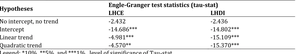
Table 4a: Cointegration Test for Lhce and Lhdi, 1980-2015
Hypotheses Engle-Granger test statistics (tau-stat)
LHCE LHDI
No intercept, no trend -2.432 -2.436
Intercept -14.686*** -14.802***
Linear trend -4.981*** -15.109***
Quadratic trend -4.570** -15.370***
Table 4a provides the results of the Engle-Granger (1987) test with LHCE and LHDI alternatively being the dependent variables. The results show that except for the no intercept no trend hypothesis, the two variables (LHCE and LHDI) are cointegrated, taking any variable as the dependent variable, under all hypotheses, i.e. the test rejects the null hypothesis of non-cointegration at 5% and 1% level of significance.
Table 4b: Cointegration Test for Lhdi and Lhce, 1980-2015
Hypotheses Phillips-Ouliaris test statistics (tau-stat)
LHCE LHDI
No intercept, no trend -11.051*** -11.052***
Intercept -14.584*** -14.691***
Linear trend -9.744*** -15.076***
Quadratic trend -8.109*** -15.275***
Legend: *10%, **5%, and ***1% level of significance of Tau-stat Source: Authors’ own computation
Table 4b presents the results of the Phillips-Ouliaris (1990) test with LHCE and LHDI alternatively being the dependent variables. The results show that the two variables (LHCE and LHDI) are cointegrated, taking any variable as the dependent variable, under all hypotheses, i.e. the test rejects the null of non-cointegration at 1% level of significance.
Table 5a: Cointegration Test for LHDI, LRPOR and LHCE, 1980-2015 Hypotheses Engle-Granger test statistics (tau-stat)
LHCE LHDI LRPOR
No intercept, no trend -2.504 -2.561 -3.168*
Intercept -17.464*** -17.338*** -3.086
Linear trend -3.793 -18.186*** -3.222
Quadratic trend -3.174 -18.172*** -3.472
Legend: *10%, **5%, and ***1% level of significance of Tau-stat Source: Authors’ own computation
Table 5a provides the results of the Engle-Granger test with lhce, lhdi and lrpor alternatively being the dependent variables. The results show that under the “no intercept, no trend” hypothesis, the variables are cointegrated only if the lrpor is selected as the dependent variable; and this at 10% level of significance. Under the “intercept” hypothesis the variables are cointegrated only if the lhce and the lhdi are selected as the dependent variables; and this at 1% level of significance. Under the “linear trend” hypothesis the variables are cointegrated only if the lhdi is selected as the dependent variable; this at 1% level of significance. Finally, under the “quadratic trend” hypothesis the variables are cointegrated only if the lhdi is selected as the dependent variable; and this at 1% level of significance.
Table 5b: Cointegration Test for LHDI, LRPOR and LHCE, 1980-2015 Hypotheses Phillips-Ouliaris test statistics (tau-stat)
lhce Lhdi lrpor
No intercept, no trend -13.325*** -13.370*** -3.078*
Intercept -16.317*** -16.235*** -3.222
Linear trend -10.560*** -17.134*** -3.399
Quadratic trend -9.254*** -17.108*** -3.788
Legend: *10%, **5%, and ***1% level of significance of Tau-stat Source: Authors’ own computation
Under the intercept, linear trend and quadratic trend hypotheses the variables are cointegrated only if the lhce and the lhdi are selected as the dependent variables; and this at 1% level of significance. In light of the cointegration test results provided in the above tables and given in the model developed earlier in this paper the lhce is the dependent variable. Furthermore, considering the intercept hypothesis for the cointegrating equation, this paper concludes that these variables are cointegrated. The next step is the estimation of the models developed earlier.
Estimation and Empirical Results: Given that a stationary linear combination exists between lhce and lhdi, the next step is to examine the error correction properties of these time series. The regression results from the three specifications discussed in (2.3) are presented as the long-run relationship (error correction mechanism) as well as the error correction model that combines the short- and long-run relationship. These results were obtained by applying the Engle-Granger two-step approach to estimate the models. The cointegrating equation, error correction mechanism or long run regression results from the three specifications are depicted in table 6.
Table 6: Cointegrating Equation, Long-Run Relationship
Dependent Variable: Household consumption expenditure - lhce
Covariates SPEC 1
(1) SPEC 2 (2) SPEC 3 (3)
Lhdi 1.050*** 0.099**x 0.100**x
L.lhce 1.163*** 1.174***
L2.lhce -0.162 -0.126
L3.lhce -0.078 -0.168
L4.lhce -0.126 -0.037
L.lhdi 0.026 0.012
L2.lhdi 0.016 0.019
L3.lhdi 0.006 -0.006
L4.lhdi 0.066* 0.042
Lrpor 0.008
L.lrpor -0.002
L2.lrpor -0.019
L2.lrpor 0.008
L2.lrpor 0.005
cons -0.653*** 0.143* -0.116
Adjusted R-squared 0.990 0.999 0.999
F-stat 13026 17078 10925
Prob-F 0 0 0
Legend: *p<0.10; **p<0.05; and *** p<0.01 Source: Authors’ own computation
The results from the three specifications of the error correction model that combine the short- and long run equations are depicted in table 7. These results show that only in specification (1) is there an adjustment to equilibrium in case of a shock, i.e. the speed of adjustment of -0.102 is negative and significant at 10% level of significance, while in both specifications (2) and (3) there is no adjustment to the equilibrium because the speed of adjustment is positive. In both specifications (2) and (3), only current, and lagged one and two HDI, as well as the constant are significant at 1%, 5% or 10% level of significance. This means that, in the short run, consumption is influenced only by these variables.
Table 7: Short-Run Relationship (Error Correction Model)
Dependent variable: household consumption expenditure (d.lhce)
Covariates SPEC 1 (1) SPEC 2 (2) SPEC 3 (3)
L.e -0.102* 0.195* 0.183
D.lhdi 0.078** 0.101** 0.102**
LD.lhdi 0.097** 0.100**
L2D.lhdi 0.097** 0.089*x
L3D.lhdi 0.040 0.051
L4D.lhdi 0.038 0.046
D.lrpor 0.005
LD.lrpor 0.003
L2D.lrpor -0.012
L3D.lrpor -0.012
L4D.lrpor -0.001
_cons 0.009*** 0.006*** 0.006***
Adjusted R-squared 0.042 0.14 0.128
F-stat 3.945 4.526 2.714
Prob-F 0.022 0.000 0.004
Legend: * p<0.10; ** p<0.05; and *** p<0.01 Source: Authors’ own estimation
The HDI long-run elasticity of 1.050 shows that, in the long run, a 1% increase in disposable income is expected to increase HCE by 1.050% points. The assessment of goodness of the models estimated is based on the normality, heteroscedasticity and the serial correlation tests on the regression residuals given that the OLS technique has been used. No issues can be raised about the normality even though the test results on all the models reject the null hypothesis of the normality of the residuals. This is because the sample used in this paper is a large one. Lumley et al. (2002) demonstrated that in large samples, the t-test and linear regression are valid for normally and non-normally distributed outcomes. The Lagrangian and Szroeter's tests with a null hypothesis (Ho) of homoscedasticity have been used to check the heteroscedasticity of the regression residuals.
Standard Errors approach that provides the heteroscedasticity and autocorrelation consistent, or HAC, standard errors (Wooldridge, 2016).
Discussion of the Results: The results displayed in table 8 indicate a slow adjustment to equilibrium since the error correction term (the coefficient on the lagged residual) is -0.1560. This coefficient is significant at 10% level of significance, meaning that at this level of significance, there is long-run causality running from disposable income to household consumption expenditure such that only 15.60% of the disequilibrium in household consumption expenditure in any time period is corrected by the following period. The results in tables 9 to 12 indicate that not almost all the estimates of the modified model are better than those of the basic model, expected the long-run estimate. The absolute income hypothesis predictions are too extreme and unrealistic because it considers only disposable income as the a priori factor expected to influence consumption expenditure. In South Africa, household consumption expenditure tends to be less subject to change than income. It is more likely to be influenced by socioeconomic background, income disparities, wealth distribution and cultural differences. Furthermore, fiscal, monetary or trade policies have to be perceived as being permanent before they can be expected to have any lasting impact on South African consumers’ consumption behavior (Pretorius & Knox, 1995). Therefore, omitting other factors can in many cases lead to contradictions between the simple Keynesian consumption model and empirical evidence. This evidence suggests that the absolute income hypothesis model is not appropriate to explain private consumption expenditure in South Africa. There is thus a need for different models that are not based on Keynes’s theory.
5. Conclusion and Recommendations
This paper examined whether the patterns of household consumption expenditure in South Africa are best determined by Friedman or Keynes’s theory. Its main objective was to investigate the relevance of the Keynesian absolute income hypothesis in explaining household consumption expenditure in South Africa since the theory assumes that disposable income is the core factor that explains household consumption expenditure. Applying the Engle-Granger two-step error correction model on time series data from the SARB from 1980 to 2015, three models were specified, namely the original, the basic and the modified models according to the absolute income hypothesis. These estimations determined the extent to which disposable income explains private consumption expenditure in South Africa, and the nature of the relationship between these variables. The empirical results indicate that private consumption expenditure in South Africa depends more on its lagged values than on absolute disposable income. Magnifying the estimates from the basic model by including the interest rate in a modified model did not yield an alternative hypothesis. Not all the coefficients on the interest rate were significant such that the Adjusted-R square compared to that of the basic model fell from 25.11% to 17.34%. These findings suggest that the Keynesian absolute income hypothesis model is not suitable to explain private consumption expenditure in South Africa because it identifies disposable income as the key element to determine household consumption expenditure.
out. This finding is in line with international studies, which argue against the attempt to explain household consumption expenditure using Friedman or Keynes’s theory.
Recommendations: Policymakers have yet to come to grips with the realities of the developing world, which do not fit with the notion that only fiscal monetary and trade, policy transmission mechanisms determine the patterns of household/private consumption expenditure. Put simply, policymakers who subscribe to either Friedman’s or Keynes’s theory underrate the factors and variables that determine such expenditure patterns. Based on the findings of this paper, a systems analysis approach is recommended to understand the determinants of household/private consumption expenditure in South Africa by putting together many systems. Multivariate models should be adopted that enable numerous variables such as culture, financial inclusion, price expectation, socio-economic background, and wealth, among others to be accounted for. This was facilitated by the emergence of the econometrics field, which raised interest in testing the claims of Keynes’s absolute income hypothesis (Alimi, 2013).
References
Alimi, R. S. (2013). Keynes absolute income hypothesis and Kuznets paradox, Munich Personal RePEc Archives, 49310.
Alogoskoufis, G. & Smith, R. (1990). On error correction models; specification, interpretation, estimation. Discussion Paper No. 6/90, Birbeck College.
Baker, M. & Orsmond, D. (2010). Household consumption trend in China. Reserve Bank of Australia Bulletin. March Quarter 2010.
Baranzini, M. (2005). Modigliani’s life-cycle theory of savings fifty years later. BNL Quarterly Review, LVIII (233-234), 109-72.
Banerjee, A., Dolado, J. J., Hendry, D. F. & Smith, G. (1986). Exploring equilibrium relationships in econometrics through static models: some Monte Carlo evidence. Oxford Bulletin of Economics and
Statistics, 48, 253-277.
Blinder, A. & Deaton, A. (1985). The time series consumption function revisited. Brookings Papers on
Economic Activity, 2, 465-521.
Campbell, J. & Mankiw, N. (1990). Permanent income, current income, and consumption. Journal of Business
and Economic Statistics, 8, 265-279.
Charemza, W. W. & Deadman, D. F. (1992). New directions in Econometric Practice, Edward Elgar Publishing Limited.
Cuthbertson, K., Hall, S. G. & Taylor, M. P. (1992). Applied econometric techniques, New York: Philip Allan. Davidson, J. E. H. & Hendry, D. F. (1981). Interpreting econometric evidence: consumers’ expenditure in the
UK. European Economic Review, 16, 177-192.
Davidson, J. E. H., Hendry, D. F., Srba, F. & Yeo, S. (1978). Econometric modelling of the aggregated time series relation between consumption and income in the UK. Economic Journal, 88(352), 661-692.
Davis, T. E. (1984). The consumption function in macroeconomic models: a comparative study. Applied
Economics, 16, 799-838.
DeBoef, S. (2001). Testing for cointegrating relationships with near-integrated data. Political Analysis, 9, 78– 94.
Engle, R. F. & Granger, C. W. J. (1987). Dynamic model specification with equilibrium constraints: co-integration and error correction. Econometrica, 55, 251-276.
Engle, R. F. & Yoo, B. S. (1991). Cointegrated economic time series: an overview with new results. In Engle R. F. & Granger C. W. J. (eds.), Long-run economic relationships: readings in cointegration, New York: Oxford University Press.
Ferber, R. (1966). Research on household behavior: Survey of economic theory. American Association and Royal Economic Society, New York and London.
Fernandez-Corugedo, E. (2004). Consumption theory. Centre for Central Banking, Bank of England. No. 23. Friedman, M. (1957). A theory of the consumption functions, Princeton, N.J: Princeton University Press. Ganong, P. & Noel, P. (2016). How does unemployment affect consumer spending? Working paper
Hall, R. (1978). Stochastic implications of the life-cycle permanent income hypothesis. Journal of Political
Economy, 86(6), 971-987
Heim, J. J. (2007). Was Keynes right? Does current year disposable income drive consumption spending? Rensselaer Polytechnic Institute Working Papers, 0710.
Heim, J. J. (2008). Consumption function. Rensselaer Polytechnic Institute Working Papers, 0805.
Hillier, B. (1991). The macroeconomic debate: Models of the closed and open economy, Oxford, New-Jersey: Basil Blackwell.
Inder, B. (1993). Estimating long-run relationships in economics. Journal of Econometrics, 57, (1-3), 53-68. Kankaanranta, P. (2006). Consumption over the life cycle: A selected literature review. Aboa Centre for
Economics, Discussion, 7.
Keynes, J. M. (1936). The general theory of employment, interest, and money. New York: Harcourt Brace. Khan, K. & Nishat, M. (2011). Permanent-income hypothesis, myopia and liquidity constraints: A case study of
Pakistan. Pakistan Journal of Social Sciences (PJSS), 31(2), 299-307.
Khan, K., Yousaf, H., Abbas, M. G., Memon Che, M. H. & Nishat, M. (2012). Permanent-income hypothesis, myopia and liquidity constraints: A case study of Pakistan. Asian Economic and Financial Review, 2(1), 155-162.
Koekemoer, R. (1999). Private consumption expenditure in South Africa: The role of price expectation and learning. PhD Thesis, Faculty of Economic and Management Sciences, University of Pretoria.
Kuznets, S. (1946). National income: A summary of findings. National Bureau of Economics Research - NBER, New York.
Kwiatkowski, D., Phillips, P. C. B., Schmidt, P. & Shin, Y. (1992). Testing the null hypothesis of stationary against the alternative of a unit root. Journal of Econometrics, 54 (13), 159-178.
Lafrance, A. & LaRochelle-Côté, S. (2011). Consumption patterns among ageing Canadians: a synthetic cohort approach. Economic Analysis Research Paper Series, Statistics Canada Catalogue No. 11F0027M, No. 067, Ottawa.
Lumley, T., Diehr, P., Emerson, S. & Chen, L. (2002). The importance of the normality assumption in large public health data sets. Annual Reviews in Public Health, 23, 151-169.
Mishkin, F. S. (2011). Monetary policy strategy: Lessons from the crisis. National Bureau of Economics Research - NBER Working Paper Series, 16755.
Modigliani, F. (1986). Life cycle, individual thrift, and the wealth of nations. American Economic Review,
American Economic Association, 76(3), 297-313.
Modigliani, F. & Brumberg, R.E. (1954). Utility analysis and aggregate consumption function: An interpretation of cross-section data. In Post Keynesian Economics, K.K Kurinara (ed) New Brunswick: Rutgers University Press.
Oke, D. M. & Bokana, K. G. (2017). Understanding the theory of consumption in the context of a developing economy. Journal of Economics and Behavioral Studies, 9(5), 219-229.
Palley, T. I. (2008). The Relative income theory of consumption: A synthesis of Keynes, Duesen berry, and Friedman model. Political Economy Research Institute, UMASS, Working Paper Number 170.
Parker, J. A., Souleles, N. C., Johnson, D. S. & McClelland, R. (2011). Consumer spending and the economic stimulus payment of 2008. National Bureau of Economic Research, Working Papers 16684.
Patterson, K. D. (1986). The stability of some annual consumption functions. Oxford Economic Papers, 38, 1-30.
Phillips, P. C. B. (1987). Time series regression with a unit root. Econometrica, 55, 277-302. Phillips, P. C. B. & Perron, P. (1988). Testing for a unit root in time series regression, Biometrika.
Phillips, P. C. B. & Hansen, B. E. (1990). Statistical inference in instrumental variables regression with I (1) processes. Review of Economic Studies, 57, 99-125.
Phillips, P. C. B. & Ouliaris, S. (1990). Asymptotic properties of residual-based tests for cointegration.
Econometrica, 58, 73-93.
Pretorius, C. J. & Knox, S. (1995). Private consumption expenditure in the macro-econometric model of the Reserve Bank, working paper.
Saikkonen, P. (1991). Asymptotically efficient estimation of cointegration regressions. Econometric Theory, 7, 1-21.
Singh, B. (2004). Modelling real private consumption expenditure – an empirical study on Fiji. Economics Department Reserve Bank of Fiji, Working Paper 2004/2005, 1-32.
Utkulu, U. (2012). How to estimate long-run relationships in economics: an overview of recent development. Vasilev, A. (2015). Modelling real private consumption expenditure in Bulgaria after the currency board
implementation (1997-2005). Zagreb International Review of Economics & Business, 18(1), 81-89. West, K. D. (1988). Asymptotic normality, when regresses have a unit root. Econometrica, 56, 1397-418. Wooldridge, J. M. (2016). Introductory Econometrics: a modern approach (6th ed), Mason, OH: South-Western
College Publishing, Cengage Learning.
Yazdan, G. F. & Merabirad, S. (2013). The testing of Hall‘s permanent-income hypothesis: A case study of Iran.
Asian Economic and Financial Review, 3(3), 311-318.