How parameter specification of an Earth system model of intermediate complexity influences its climate simulations

R E S E A R C H A R T I C L E

Open Access

How parameter specification of an Earth

system model of intermediate complexity

influences its climate simulations

Yuhan Shi

, Wei Gong

, Qingyun Duan

, Jackson Charles

, Cunde Xiao

and Heng Wang

Abstract

Earth system models (ESMs) consist of parameterization schemes based on one’s perception of how the Earth system functions. A typical ESM contains a large number of parameters (i.e., the constants and exponents in the parameterization schemes) whose specification can have a significant impact on an ESM’s simulation capabilities. Sensitivity analyses (SA) is an important tool for assessing how parameter specification influences model

simulations. In this study, we used an Earth system model of intermediate complexity (EMIC)—LOVECLIM as an example to illustrate how SA methods can be used to identify the most sensitive parameters that control the simulations of several key global water and energy cycle variables, including global annual mean absolute surface air temperature (TG), precipitation and evaporation over the land and over the oceans (PL,PO,EL,EO), and land

runoff (_RL). We also demonstrate how judiciously specifying model parameters can improve the simulations of

those variables. Three SA methods MARS, RF, and sparse PCE-based Sobol’method were used to evaluate a pool of 25 adjustable parameters chosen from land, atmosphere, and ocean components of LOVECLIM and their results were intercompared to ensure robustness of the results. It is found that with different parameter specification,_TG

can vary from 10 to 20 °C, and the values ofPL,PO,EL, andEOcan change by more than 100%. An interesting

observation is that the value ofRLvary from 13,000 to 35,000 km3, far below the observed climatological value of

40,000 km3, indicating a model structural deficiency in representing land runoff by LOVECLIM which must be corrected to obtain more reasonable global water budgets. We also note that parameter sensitivities are significantly different at different latitudes. Finally, we showed that global water and energy cycle simulations can be significantly improved by even a crude automatic parameter tuning, indicating that parameter optimization can be a viable way to improve ESM climate simulations. The results from this study should help us to understand the parameter uncertainty of a full-scale ESM.

Keywords:Parameter sensitivity analysis, Earth system model of intermediate complexity, LOVECLIM, Parametric

uncertainty

Introduction

Earth system models (ESMs) are an indispensable tool for gaining an understanding on how the climate system works and how its various components such as land, at-mosphere, and oceans interact with each other. They have been used extensively to simulate the past and future

climatic processes and events. The simulation and predict-ive capabilities of ESMs are influenced by several factors such as the specification of model forcings, the specifica-tion of initial and boundary condispecifica-tions, and the represen-tation of model physics. In the past, much attention has been paid to develop various models of different complex-ities. Over the recent years, researchers become increas-ingly aware that tuning is an essential aspect of climate modeling (Hourdin et al.2017). The purpose of tuning is to reduce the distance between model results and the ob-served climate by adjusting the values of various parame-ters. It has been shown that the simulation capability of a

© The Author(s). 2019Open AccessThis article is distributed under the terms of the Creative Commons Attribution 4.0 International License (http://creativecommons.org/licenses/by/4.0/), which permits unrestricted use, distribution, and reproduction in any medium, provided you give appropriate credit to the original author(s) and the source, provide a link to the Creative Commons license, and indicate if changes were made.

* Correspondence:[email protected]

1_{State Key Laboratory of Earth Surface Processes and Resource Ecology,} Faculty of Geographical Science, Beijing Normal University, Beijing 100875, China

climate model may be enhanced significantly by adjusting the values of even one or two of its model parameters (Collins et al. 2006; Gent et al. 2011; Sanderson et al. 2008; Tebaldi and Knutti2007; Williamson et al.2013).

In fields such as hydrology and engineering, parameter tuning or optimization methods have been commonly used to estimate model parameters. However, parameter optimization of climate models is an enormous compu-tational task for the following reasons: (1) optimization of climate model parameters is a high-dimensional prob-lem because climate models usually contain a large number of adjustable parameters (dozens or even hun-dreds of parameters), and the number of model experi-ments to optimize those parameters is exponentially proportional to the dimensionality; (2) climate models simulate many climatic variables (e.g., temperature, pre-cipitation, evaporation, wind speed, and pressure), and the optimization problem must be framed as a multi-objective optimization problem, which further increases the number of model experiments needed to identify op-timal parameter solutions; and (3) climate models are expensive to run because they must be run globally and cover time span over many years. Even with today’s most advanced supercomputers, the amount of computational resources required for optimizing the parameters of a climate model can still be prohibitive.

Climate models vary in complexity from simple concep-tual models to sophisticated earth system models (Claussen et al.2002; Eby et al.2013). Simple conceptual models are useful in developing and exploring the variability of individ-ual processes in the climate system. However, these models only describe a very limited number of processes and vari-ables. Current state-of-the-art Earth system models (ESMs) provide very detailed descriptions of the Earth system, in-cluding more feedbacks and processes. Because of their complexities, the number and length of simulations that can be conducted are limited by the availability of computa-tional resources and it is not practical to perform parameter estimation exercises on full-scale ESMs. Another class of models, known as the Earth system models of intermediate complexity (EMICs), helps bridge the gap between the sim-plest and most complex climate models (Claussen et al. 2000). EMICs provide a fairly complete description of the Earth system, including almost all components of the Earth system, but this often occurs in an idealized manner or at a lower resolution than the models described above. To ex-plore the various feedbacks among different components of the climate system, EMICs simulate long-term climate changes with parameterization schemes to simplify the vari-ous processes and details of the climate system. These models are usually applied to certain scientific questions, such as understanding climate feedbacks on millennial time scales or exploring sensitivities in which long model inte-grations or large ensembles are required (Claussen et al.

2002; Petoukhov et al. 2005). To a certain extent, EMICs combine the advantages of simple conceptual models and Earth system models and overcome their disadvantages. As computing power increases in the future, this model class will continue to advance in terms of resolution and com-plexity. This study uses an EMIC model as an example to study how parameter specification affects climate model simulations and to explore potentials for improving climate model simulation through parameter perturbations.

Despite the differences between EMICs and ESMs in model conceptualization and structures, we hope the ex-periences with parameter specification methods (such as uniform sampling, sensitivity analysis, etc.) of simple and computational affordable EMICs can be applied to full-scale ESMs to improve ESMs performance with less computational resources.

In our previous studies (Duan et al. 2017; Gan et al.

2014; Gong and Duan2017; Gong et al.2015; Gong et

al.2016a; Gong et al. 2016b), an uncertainty quantifica-tion (UQ) framework was developed to quantify the un-certainty of large, complex dynamic system models, such as land-surface, weather, and climate models, which in-clude many physical processes and cost a substantial amount of computational resources to run. The uncer-tainty quantification framework includes the following steps: (1) using parameter screening to reduce the num-ber of adjustable parameters, (2) building a surrogate model to emulate the response surfaces of the original model to the variation in the adjustable parameters, and (3) running the surrogate model with the sensitive pa-rameters to optimize the original model. Sensitivity ana-lysis (SA) methods have been shown to be very effective for parameter screening to determine the parameters which exert significant influence on climate model simu-lations of interested variables (Gutiérrez et al. 2009;

Ratto et al. 2012; Shahsavani and Grimvall 2011). SA

methods use a design of experiment (DoE) approach to sample model parameters within a feasible range and quantify the influence of each adjustable parameters to the model output. The parameters that have significant influence to model outputs are screened out as import-ant parameters. So far, there have been numerous stud-ies that have used SA methods to examine the parametric sensitivity of hydrology (Gupta and Razavi 2018; Ricciuto et al.2018; Sarrazin et al.2016; Zadeh et al. 2017) and land-surface models (Bastidas et al. 2006; Liu et al. 2004; Santanello Jr et al. 2011; Xiong et al.

2010), numerical weather prediction (NWP) models (Di

et al. 2015; Johannesson et al. 2014; Quan et al. 2016),

and climate models (Edwards and Marsh2005; Fanning

and Weaver 1997; Murphy et al. 2004; Neelin et al.

2010).

the simulation of interested climatic variables such as surface air temperature, global water budget components including precipitation, evaporation over land and ocean, and runoff over land simulated. Here, we chose an EMIC named LOVECLIM as an example to illustrate the effectiveness of SA methods. Then we evaluated the perturbed parameters and find some individual param-eter sets have better agreements to some aspects of

se-lected climatic variables, implying that automatic

parameter tuning has the potential to further improve the performance of LOVECLIM.

We choose to focus on sensitivity of parameter specifi-cation on the simulations of surface air temperature and global water balance components in this study because those climatic variables have the most direct impacts on human beings and on Earth’s sustainability. Recent IPCC assessment reports suggested that current GCMs per-formed reasonably well in capturing the global mean temperature trend over the last 150 years. However, there was a persistent discrepancy between different GCMs in terms of global mean absolute temperature simulations, which differed by as much as 3 °C in both

IPCC AR4 and IPCC AR5 (IPCC 2007; IPCC 2013;

Mauritsen et al.2012). All climate models are supposed to confirm to physical laws such as the conservation of mass and energy and water’s freezing point always being

0 °C given Earth’s condition. When the global mean

temperature simulations differ by 3 °C or more, the fol-lowing issues would arise. The involved models would contain very different land states (i.e., water may be in li-quid state more likely in one model, while in frozen state in another) and this would ultimately affect the land hydrological processes. In addition, the land-atmosphere interactions would be very different, leading to different global water and energy budgets. Therefore, absolute global surface air temperature is an important metric for summarizing the state of the global climate (Hansen et al.2006). Parameter specification can strongly affect the simulation of the hydrological cycle on Earth (Chahine 1992), which in turn influences Earth’s simulated climate in a variety of ways. The exchanges of moisture and heat

between the atmosphere and Earth’s surface

fundamen-tally affect the dynamics and thermodynamics of the

cli-mate system (Jones 2014). According to the

Clausius-Clapeyron relation, the specific humidity increases expo-nentially with temperature under a background of

cli-mate change (Allen and Ingram 2002). The

Clausius-Clapeyron relation states that the water-holding capacity of the atmosphere increases by approximately 7% for every 1 °C rise in temperature. Incorrect simulation of hydrological cycle would lead to incorrect simulation of extreme climatic events, such as extreme precipitation and drought. By choosing global mean absolute surface air temperature and global water budget components as

the parameter optimization targets (Eyring et al. 2016; Mauritsen et al. 2012), we hope to achieve better simu-lated global climate patterns. This article includes five

sections: Introduction gives the background to the

re-search; Methods and tools introduces the sampling

method, sensitivity analysis method, and tools used in

this study; Model and parameters introduces the basic

information for LOVECLIM and the adjustable

param-eter information; Results and discussion analyzes and

discusses the experimental results; andConclusions pro-vides the summary and conclusions.

Methods and tools

The purpose of a sensitivity analysis (SA) is to quantify the influence of different parameters on the model out-puts of interest. The SA process works as follows: (1) identify the adjustable parameters and their feasible ranges, (2) generate samples in high-dimensional param-eter space and run the model with those samples, and (3) choose one or more appropriate SA methods and ob-jective functions to quantify the parameter sensitivity with the input parameters and output variables. The ad-justable parameters and their feasible ranges are

pre-sented in “Results and discussion” section. Below, we

provide a brief description of the sampling method, SA method and tools used in this study.

Sampling method

In previous research (Gong et al. 2016a), we have found that the good lattice points (GLP) method can generate relatively more uniform samples than other methods, such as the widely used Monte Carlo and Latin Hyper-cube methods; therefore, we choose this sampling method in this study. The GLP method is also called the

Korobov lattice rules (Hlawka 1962; Korobov 1959a;

Korobov 1959b; Korobov 1960), which is a number

theory-based quasi-Monte Carlo (QMC) method. The GLP design is generated by the following equations:

qki¼khiðmod nÞ

xki¼ð2qki−1Þ=n ;k

¼1;⋯;n;i¼1;⋯;s

ð1Þ

wheren represents the number of samples,s represents the number of dimensions,xkirepresents the coordinate of the kth sample point in the ith dimension,qki repre-sents an internal variable, and hi represents an element in the generating vector. The range of coordinate xki is restricted to [0,1]. The greatest common divisor of hi andnis 1. The vector (n:h1,⋯,hs) is called the

generat-ing vector. If the point set Pn= {xk= (xk1,⋯,xks),k= 1,

less samples and, thus, save computational resource costs for the sensitivity analysis.

Sensitivity analysis methods

This study employed two qualitative SA methods to per-form the parameter screening: multivariate adaptive re-gression splines (MARS) and random forests (RF). Moreover, to validate the parameter screening results obtained by the qualitative methods, the sparse

polyno-mial chaos expansion (PCE)-based Sobol’method (SPC)

was applied to compute the total effects of the parameters.

Multivariate adaptive regression splines

The MARS method (Friedman 1991) is a generalization

of the stepwise linear regression, and it is suitable for high-dimensional problems. We call the two expanded piecewise linear basis functions (x−t)+ and (t−x)+ used

in the MARS the reflected pair, where t is a constant

called the knot. Our aim is to form reflected pairs for

each parameter Xj with knots at each xij value for that

input. Therefore, the collection of basic functions is

C¼ Xj−t

þ; t−Xj

þ

n o

t∈ x1j;x2j;⋯;xNj

;j¼1;2;⋯;p

ð2Þ

whereNrepresents the number of samples,prepresents the total number of adjustable parameters, andXj repre-sents the j-th adjustable parameter.

The MARS method includes a forward procedure and backward procedure. First, we build a forward stepwise linear regression using the functions from the set C and its products. Thus, the model has the form

f Xð Þ ¼β0þ

XM

m¼1

β_mhmð ÞX ð3Þ

where β0 represents the intercept, βm represents the slope, andf(X) corresponds to the predicted value of the observable variables (i.e., the output variables), such as temperature or precipitation. Bothβ0andβmare regres-sion coefficients in the regresregres-sion model, and their values are estimated by minimizing the residual sum-of-squares. Each hm(X) is a function of C or a product of two or more similar functions, and M represents the number of functions. Equation (3) is a regression model that can predict the value of the observable variable yi with the parameter valueX.

This model typically overfits the data; therefore, a backward deletion procedure should be applied. The term whose removal causes the smallest increase in the residual squared error is deleted from the model at each stage to produce an estimated best model (fbλ) for each

size (number of terms) of λ. The MARS procedure uses

generalized cross-validation (GCV) to estimate the opti-mal value ofλ:

GCVð Þ ¼λ

Xn

i¼1

yi−fbλð Þxi

2

1−Mð Þλ =n

ð Þ2 ð4Þ

wherenrepresents the number of observations,yi repre-sents theith observation,fbλðxiÞrepresents the estimated value of yi, and M(λ) represents the number of effective parameters in the model.

The importance of the removed variable is measured by the increase in GCV values between the pruned model and overfitted model (Steinberg et al. 1999). The greater the increase in GCV is, the more important the removed variable.

The MARS method can also be used as a

surrogate-model. Shahsavani et al. (2010) showed that using the

MARS surrogate model to replace the original dynamic model can provide acceptable estimates of the total sen-sitivity indices at much lower costs.

Random forest

The random forest (RF) is a very efficient and increas-ingly popular machine-learning algorithm for both clas-sification and regression problems that was introduced by Breiman (2001). RFs are a substantial modification of

bagging (Breiman 1996) that construct multiple trees

(i.e., forests) using bootstrap sampling, and their deci-sions are averaged. The main difference between RFs and bagging is that a RF searches a randomized subset of input variables to determine a split at each node, which is the reason why it is called “random” forests. The basic principle of RFs is a group of weak learners that can come together to form a strong learner.

The random forest algorithm is as follows:

1. Extract a bootstrap sample, Z*, of sizeNfrom the training data.

2. For each of the bootstrap samples, grow a random forest tree by recursively repeating the following steps ((a) to (c)) for each terminal node of the tree until the minimum node sizenminis reached.

(a) Randomly selectmvariables from the total p variables, wherem< <p.

(b) Among the m variables, pick up the best variable/split point.

(c) Split the node into two daughter nodes using the best split.

3. Predict the new data by aggregating the predictions of theNtrees.

avoid overfitting because of the law of large numbers, and RFs can be used to identify important factors. The total number of splits can determine the importance of this variable. The more splits the variable has, the more sensitive the variable is.

Sparse PCE-based Sobol’method

The Sobol’ method (Sobol’ 1993) is a quantitative SA

method based on the principle of variance decompos-ition and can be applied to nonlinear, nonmonotonic mathematical models. Its core idea is to decompose the total variance of the objective function into the variance of a single parameter and the variance of the interaction between parameters. By comparing the three methods of

PEST, RSA, and ANOVA with the Sobol’method, Tang

et al. (2006) considered that the Sobol’ method is more robust and superior to other methods in both single ob-jective and multi-obob-jective sensitivity analyses.

Suppose the problem can be considered as y=f(X) =

f(X1,⋯,Xk), whereyrepresents the objective function of the model output (e.g., the root mean square errors of the simulated values and default values), andX= (X1,⋯,

Xk) is the vector of thekmodel factors (e.g., parameters) to be used to control the behavior of the model. Without loss of generality, each parameterXiwas supposed to be feasible in range [0, 1]. Our purpose is to explore how much of the total variance_D(_y) in_ycan be explained by variability in the factors of X. The Sobol’ method com-putes this by decomposing the function f(X) into terms of increasing dimensionality, such that each successive dimension represents how much the interaction between parameters increases.

f Xð 1;X2;⋯XkÞ ¼f0þ

Xk

i¼1

fið ÞXi

þ X

1≤i<j≤k

f_ij Xi;Xj

þ⋯

þf1;2;⋯;kðX1;⋯;XkÞ ð5Þ

wheref0is constant that equals to the expected value of

f(X), fi(Xi) is a function of the ith parameter,fij(Xi,Xj) is a function of the ith and jth parameters, etc. The inte-grals of the decomposed functions (also called sum-mands)fi(Xi),fij(Xi,Xj),⋯, f1, 2,⋯,k(X1,⋯,Xk) are equal

to zero:

Z 1

0 fi1;i2;⋯;is Xi1;⋯;Xis

ð Þdxik ¼0if 1≤k≤s ð6Þ

All the summands can be computed recursively like this:

f0¼ Z1

0 …

Z1

0

fð ÞX dX;

fið Þ ¼Xi Z1

0 …

Z1

0

fð ÞX dXi−f0;

fij Xi;Xj

¼ Z1 0 … Z1 0

fð ÞX dXij−f0−fið ÞXi −fj Xj ;

ð7Þ

The notation ~ means the parameters are excluded like thisX_~i=(X1, …,Xi−1,Xi+ 1, …,Xk).

The total variance of the functionf(X) is defined as:

D Yð Þ ¼

Z 1

0

⋯

Z 1

0 f 2_{ð ÞX}

dX−f20 ð8Þ

And the contribution of a generic term fi1;⋯;isð1≤i1

<⋯<is≤kÞto the total variance can be written as

Di1;⋯;is¼

Z 1

0

⋯

Z 1

0

f_i21;⋯;isðXi1;⋯;XisÞdXi1⋯dXis

ð9Þ

whereDi1;⋯;is denotes the partial variance corresponding

to (_i1,⋯,_is), the integer _s is called the order or the di-mension of the index. On this basis, the total variance of the output variableYcan be decomposed into of all par-tial variances:

D yð Þ ¼X

k

i¼1

Diþ X

1≤i<j≤k

Dijþ⋯D1;2;⋯k ð10Þ

whereDirepresents the contribution of factorXitoD(y) andDijrepresents the contribution of the interaction be-tween factors Xi and Xj. Similarly, D1, 2, ⋯k represents

the contribution by the interaction of k factors. The Sobol’sensitivity index of s factors is defined as

Si1;⋯;is ¼

Di1;⋯is

D Yð Þ;1≤i1<⋯<is≤k ð11Þ

and the sum of all Sobol’sensitivity indices equals to 1:

1¼Xn i¼1Siþ

X

1≤i<j≤kSijþ⋯þS1;2;⋯;k ð12Þ In the Sobol’ method, Si=Di/D(Y) is the main effect (i.e., the first-order effect) of the ith variable, and Sij=

Dij/D(Y) is the interaction effect (i.e., second-order ef-fect) of theith andjth variables.STi= 1−D~i/D(Y)

repre-sents the total sensitivity of the ith variable, where D~i

is the sum of the first-order effect (main effect) and all

other order effects involving Xi, including two factor

interaction effects and all higher order interaction effects.

Traditionally, the Sobol’ indices are evaluated with

Monte Carlo sampling, and to obtain an accurate es-timation the number of sample size (equals to

num-ber of model simulation) is usually very high. Sobol’

method is too expensive for computationally expen-sive models. Using surrogate model to replace the

ex-pensive dynamic model in Sobol’ method can

significantly save the computational resources. Sudret

(2008) proposed a post-processing of polynomial

chaos expansions (PCE) that can directly obtain the

Sobol’ sensitivity indices from the polynomial

coeffi-cients of PCE. Comparing with the Monte Carlo

sam-pling and the PCE-based way of computing Sobol’

indices, Sudret’s PCE-based method cost less

compu-tational resources and can obtain more accurate result.

Here is a brief introduction to sparse PCE Sobol’

method. Considering a random vector with independent components X∈ℝkand a computational model Y=f(X) with finite variance, the polynomial chaos expansion of

f(X) is defined as:

Y¼ fð Þ ¼X X α∈ℕk

λαΨαð ÞX ð13Þ

where theΨ_α(X) are multivariate polynomials orthonor-mal with respect to the distribution of X , α∈ℕk is a vector of indices that identifies the components of the multivariate polynomialsΨ_α, and the correspondingλ_α∈

ℝ are the coefficients of each orthonormal. Equation

(13) is usually referred to as the polynomial chaos ex-pansion (PCE) of Y. In realistic applications, the

trun-cated polynomial chaos expansions are usually

introduced to retain only a finite number of PCE terms:

fð ÞX ≈ fPCð Þ ¼X X α∈A

λαΨαð ÞX ð14Þ

In this equation,Ais the set of vectors of selected in-dices of multivariate polynomials. This equation is called the full polynomial chaos. The key of constricting a sparse polynomial chaos (SPC) is to determine the coef-ficients λ_α of each term. In this paper, we used the or-thogonal matching pursuit (OMP) originally proposed

by Pati et al. (1993) to determine the polynomial

coefficients.

The Sobol’indices can be computed from the

polyno-mial coefficientsλ_αdirectly as follows:

E fð ð ÞX Þ≈λ0; V fð ð ÞX Þ≈ X

α∈A

α≠0

λ2

α;

Si≈

1

V fð ð ÞX Þ X

α∈A_Si λ2

αwithASi¼fα:αi>0;αk¼0 fork≠ig;

STi≈

1

V fð ð ÞX Þ X

α∈A_STiλ

2

αwithASTi¼fα:αi>0g;

ð15Þ

whereA_Si is the set of indices vectors that only have the

ith factor, while A_STi is the set of indices vectors that have the ith factor and maybe also others, E(f(X)) and

V(f(X)) are mean and variance off(X), respectively. The confidence intervals of Sobol’ sensitivity indices can be

estimated with the bootstrap method (Efron1979).

Tools

The Uncertainty Quantification Python Laboratory (UQ-PyL) (Wang et al. 2016) is a flexible software platform designed to quantify uncertainties in large complex dy-namical models. UQ-PyL integrates different kinds of UQ methods, including experimental design, statistical analysis, sensitivity analysis, surrogate modeling, and parameter optimization. In this study, we used the unre-leased developed version of the UQ-PyL for the experi-mental design and sensitivity analysis. The MARS algorithm is available from the open-source software py-earth (https://github.com/scikit-learn-contrib/py-earth),

the Sobol’ method implemented in SALib (https://

github.com/SALib/SALib), and the Sparse PCE-based

Sobol’ method we used comes from UQLab (https://

www.uqlab.com/).

Model and parameters

We selected an EMIC called LOVECLIM (Goosse et al. 2010) to explore the parameter sensitivity of its various output variables. LOVECLIM has five components: the

atmospheric model ECBILT (Opsteegh et al. 1998), the

sea-ice and ocean model CLIO (Goosse and Fichefet

1999), the terrestrial biosphere model VECODE (Brovkin

et al.1997), the ocean carbon-cycle model LOCH

(Mou-chet and François 1996), and the ice-sheet model

AGISM (Huybrechts 2002). Originally, the ECBILT and

CLIO were coupled in the late 1990s (Goosse et al. 2001; Goosse et al.2002). This version is followed by the ECBILT-CLIO-VECODE model, which includes the ter-restrial biosphere (Renssen et al. 2003; Renssen et al.

2005). The LOVECLIM acronym

because they are not necessary for the processes investi-gated here, they are not public, and their use is subject to permission.

Loutre et al. (2011) and Goosse et al. (2007) explored the impact of parameter changes on the performance of the LOVECLIM with various parameter sets. Based on their experience on selecting adjustable parameters and the physical meanings of the parameters, 25 parameters in LOVECLIM are chosen as the adjustable parameters in this study. Previous studies have shown that approxi-mately ± 30% perturbations in the default parameter values were suggested for the sensitivity and uncertainty

analyses (Tan et al.2017). One way to make the

reduc-tion of model large-scale biases and the parameterizareduc-tion development processes more“in tune”is by deriving an acceptable range of parameter values instead of a single value from the aforementioned process studies and use this range when tuning global simulations (Hourdin et

al. 2017). Based on our experience and the physical

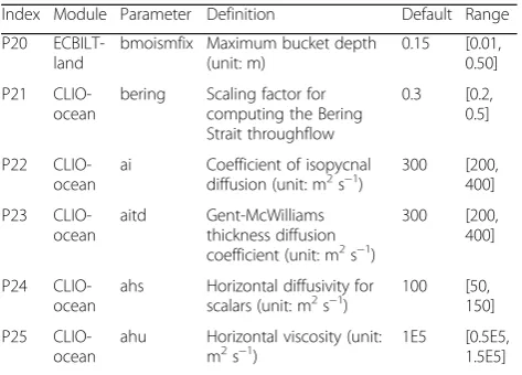
meanings of the adjustable parameters, we determined the feasible ranges of the parameters, as shown in

Table 1. These adjustable parameters can be classified

into three categories: atmosphere, land, and ocean. A rough rule of thumb about the sample size is that at least 10 ×nsample points are needed to identify the key factors (i.e., parameters), wherenrepresents the number

of experimental factors (Levy and Steinberg 2010). In

this study, 25 × 10 = 250 samples were generated with the GLP method.

Results and discussion

Experiment on the perturbed parameters

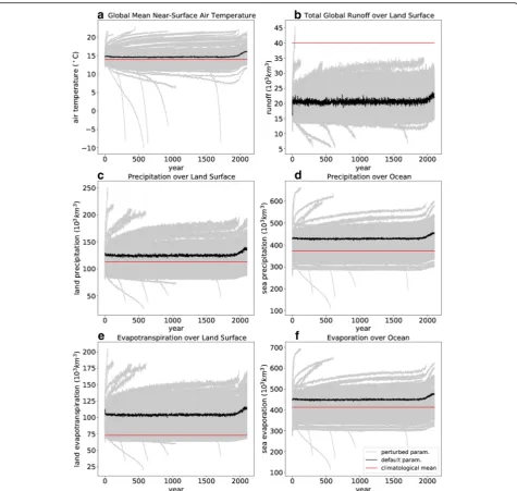
We performed climate simulations using LOVECLIM over a 2100-year period from 1 to 2100 C.E. using the default model parameters as treat the simulation as con-trol run. We then run LOVECLIM model 250 times using sampled parameter sets generated by the GLP method described in“Methods and tools”section for the same period. We chose six output variables as the ana-lysis objects: global mean near-surface air temperature

(TG), total global runoff over land surface (RL), total

pre-cipitation over land surface and ocean (PL and PO), and

total evaporation over land surface and ocean (EL and

EO).

According to the analysis of these output variables, we found that 189 simulation results are valid, while the other simulations drifted or crashed during the

simula-tion period. We have also examined the trends ofTG in

these 189 simulations over the period 1001 to 1800 C.E., the maximum absolute value of the trends is 0.00291 °C/ year, which is within a reasonable range. Figure1 shows all of the time series of the output variables simulated with perturbed parameters, with the redline denoting the climatological means of observations and the black

line denoting the ensemble mean. The climatological

means of observations of TG used is the

twentieth-century average provided by NOAA (https://www.ncdc.

noaa.gov/sotc/global/201613), and the global water budget components RL, PL, PO, EL, and EO is obtained from the work by Trenberth et al. (2007) based on ERA-40 reanalysis data. Their ensemble spreads span across a wide range, and the differences between the highest values and lowest values are significant. From Fig. 1a–f, the maximum ranges between the highest values and

lowest values are 10.35 °C, 22.16 × 103 km3, 88.67 ×

103 km3, 264.82 × 103 km3, 84.17 × 103 km3, and 269.61 × 103 km3, respectively. Note that the ensemble spreads of some variables covered the climatological values, including TG, PL, PO, EL, and EO. However, the

observed climatological mean of RL is out of the range

of the ensemble spread, indicating a model structural problem, which will be elaborated more in details later.

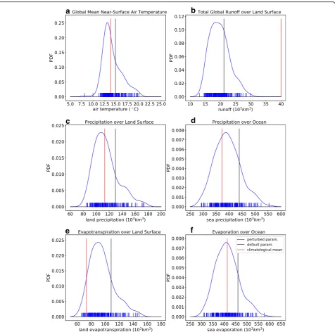
Figure2shows the probability density function for the results of the output variables using perturbed parame-ters and compares them with the simulation results using the default parameter and climatological mean values. Compared with the climatological mean, the simulation with default parameters has a warming bias of approximately 1 °C, and PL, PO, EL, and EO are all positively biased, indicating a more active hydrological cycle than observed occurred. Compared with the ERA-40 reanalysis data, RL has a significant negative bias and

ELhas a strong overestimation. Comparing with the real world, the runoff over land surface is too little, while evapotranspiration over land is too much. The positively

biased EL leads to biased surface latent heat flux and

may possibly have some influence of global energy balance.

unsaturated. Consequently, in hydrological models, usu-ally a leaky bucket (or multiple leaky buckets) are used to describe this process. If the bucket is not leaky, all of the water must take part in evapotranspiration, similar to a “shallow sea”scenario, and runoff cannot be gener-ated from half-filled bucket. The oversimplified LBM model may lead to negatively biased runoff, overesti-mated evapotranspiration and latent heat flux over land, and biased thermodynamic discrepancy between land and ocean. Too much water involved in land evapotrans-piration may possibly be the reason why the simulated global hydrological cycle is stronger than that of the real world, as it pumps more water into the atmosphere. Be-cause of the complex interactions among the atmos-phere, land, sea, and biosatmos-phere, the influence of a biased hydrological process may distort the global climate and lead to biased future climate projections.

The overall sensitivity analysis results

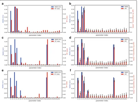
The simulation results of year 1951 to 2000 C.E. were selected for sensitivity analysis. Figure 3 shows the SA results for three output variables: global mean surface temperature, total global precipitation, and total global evaporation with three SA methods: the MARS, random

forest, and sparse PCE-based Sobol’methods (SPC). The

sensitivity scores of the 25 parameters are normalized to [0, 1]. The blue columns in the figures represent the SA results (MARS GCV score) of the MARS method; the red columns in subfigures (a) (c) (e) represent the SA re-sults (RF score) of the random forests, while the red col-umns in subfigures (b) (d) (f ) represent the SA results (Sobol’indices) of the SPC method. As shown in Fig.3a, b, the parameters P1, P3, and P4 are very sensitive to surface temperature with the three SA methods, while the other parameters are not sensitive to surface temperature within the adjustable range of parameters we chose in this study. For the total global precipitation

Table 1List of selesscted adjustable parameters and their ranges of LOVECLIM

Index Module Parameter Definition Default Range

P1 ECBILT-atm

ampwir Scaling coefficient for the longwave radiation scheme

(amplw)—general value (excluding the equator area).

1 [0.5, 1.5]

P2 ECBILT-atm

ampeqir Scaling coefficient for the longwave radiation scheme (amplw)—for the equator area between 15° S and 15° N.

1.8 [1.0, 2.5]

P3 ECBILT-atm

expir Exponent for the longwave radiation scheme 0.4 [0.2, 0.6] P4 ECBILT-atm

relhmax Precipitation also occurs if the total precipitable water below 500 hPa is above this relevant threshold.

0.83 [0.50, 0.90]

P5 ECBILT-atm

cwdrag Drag coefficient to compute wind stress

2.1E-3 [1.0E-3, 4.0E-3]

P6 ECBILT-atm

cdrag Drag coefficient to compute sensible and latent heat fluxes

1.4E-3 [1.0E-3, 2.0E-3]

P7 ECBILT-atm

uv10rfx Reduction in wind speed between 800 hPa and 10 m

0.8 [0.7, 0.9]

P8 ECBILT-atm

dragan Rotation of the wind vector in the boundary layer (unit: degree)

15 [10, 20]

P9 ECBILT-land

alphd Albedo of snow 0.72 [0.60, 0.90]

P10 ECBILT-land

alphdi Albedo of bare ice 0.62 [0.50, 0.80]

P11 ECBILT-land

alphs Albedo of melting snow 0.53 [0.30, 0.60]

P12 ECBILT-land

albice Albedo of melting ice (general)

0.44 [0.30, 0.60]

P13 ECBILT-land

albin Albedo of melting ice (Arctic)

0.44 [0.30, 0.60]

P14 ECBILT-land

albis Albedo of melting ice (Antarctic)

0.44 [0.30, 0.60]

P15 ECBILT-land

cgren Increase in snow/ice albedo under cloudy conditions

0.04 [0.01, 0.10]

P16 ECBILT-atm

corAN Reduction in precipitation over the Atlantic (North)

−0.085 [−0.10,

−0.05]

P17 ECBILT-atm

corAS Reduction in precipitation over the Atlantic (South)

−0.085 [−0.10,

−0.05]

P18 ECBILT-atm

corAC Reduction in precipitation over the Arctic

−0.25 [−0.30,

−0.20]

P19 ECBILT-land

evfac Maximum evaporation factor over land

1 [0.5, 1]

Table 1List of selesscted adjustable parameters and their

ranges of LOVECLIM(Continued)

Index Module Parameter Definition Default Range

P20 ECBILT-land

bmoismfix Maximum bucket depth (unit: m)

0.15 [0.01, 0.50]

P21 CLIO-ocean

bering Scaling factor for computing the Bering Strait throughflow

0.3 [0.2, 0.5]

P22 CLIO-ocean

ai Coefficient of isopycnal diffusion (unit: m2s−1)

300 [200, 400] P23 CLIO-ocean aitd Gent-McWilliams thickness diffusion coefficient (unit: m2s−1)

300 [200, 400]

P24 CLIO-ocean

ahs Horizontal diffusivity for

scalars (unit: m2_s−1₎ 100 [50,_150]

P25 CLIO-ocean

ahu Horizontal viscosity (unit: m2s−1)

and total evaporation, the results of the MARS, RF, and SPC methods are consistent with each other, and the parameters P1, P2, P3, P4, P6, and P19 are

sensi-tive. The confidence intervals of Sobol’ indices have

also been estimated with bootstrap method. The 25% and 75% quantiles of each indices were shown in

Fig. 3b, d, f. Comparing with the magnitude of Sobol’

indices, the range of confidence intervals are relatively small, leading to a high confidence of the result of sensitivity analysis. Although there are some discrep-ancies in the order of sensitivity scores, three differ-ent methods have reached a consensus that which

parameters are sensitive and which are not. In gen-eral, we can conclude that the three methods produce similar results with satisfying confidence to make a solid conclusion.

Furthermore, we have also evaluated the parameter sensitivity of pre-industrial age (1701 to 1800 C.E.). Gen-erally speaking, the sensitivity analysis results are similar to that of current age (1951 to 2000 C.E.). All of the fig-ures presenting sensitivity analysis results of both pe-riods can be found in the Additional file 1: Figures S1– S12. In the following parts of this paper, only results of current age (1951 to 2000 C.E.) were presented.

Sensitivity analysis results of global mean output variables

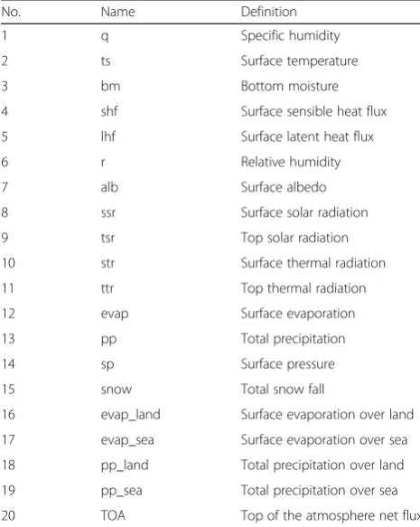
Figure 4 shows the sensitivity results of the global

mean values of 20 output variables (Table 2) to 25

adjustable parameters provided by the SPC method. We find that parameters P1, P3, P4, and P19 are sen-sitive for almost every variable. Parameters P2, P5, P6, and P9 are sensitive for 8–15 variables. All other parameters are slightly sensitive for the selected out-put variables.

Referring to the parameter list in Table1, we find that the sensitive parameter P1 and P2 are scaling coefficient for the longwave radiation scheme, which controls the radiation due to the anomaly of humidity. The param-eter P3 is the exponent of humidity anomaly for the longwave radiation scheme. The sensitivity of the above three parameters confirms our prior knowledge that the longwave radiation from atmospheric water vapor is an important factor in the global climate system. The P4

parameter, which is about microphysics and

a

b

c

d

e

f

precipitation, can also influence many aspects of global climate. As the only global microphysics parameter, P4 controls the amount of atmospheric water vapor and precipitation worldwide, and consequently influence the global energy balance. The drag coefficients P5 (for wind stress) and P6 (for sensible and latent heat fluxes) are also important because they played an important role in land-atmosphere interactions. P6 is more important be-cause the sensible and latent heat flux can influence both energy and water balance. The parameters P1 to P6 are about global water and energy balance in the atmos-phere module, and we have confirmed that they have strong influence to the global climate simulation. The snow albedo P9 can influence radiation and temperature terms, confirming that the parameterization of snow cover is important for climate modeling. The maximum evaporation factor over land (P19), which can adjust the evapotranspiration amount over land surface, is also

sen-sitive to many output variables, indicating the

importance of land surface evapotranspiration process to the global climate system.

However, some parameters that are considered to be also important, or at least functional, were shown to be only slightly sensitive in our results. The snow/ice pa-rameters such as the albedos of bare ice (P10), melting snow (P11), melting ice (P12, P13, P14) and correct fac-tor of snow/ice albedo under cloudy conditions (P15), the precipitation and microphysics regional reduction factors P16~P18, and all of the ocean module parame-ters P21~P25. The most unexpected result is that all of the ocean parameters are only a little sensitive in the time scale of thousands of years, which somehow dis-agree with our prior knowledge that the ocean processes controls the climate variability in the time scale of hun-dreds to thousands of years. All of the three sensitivity analysis methods, namely MARS, RF, and SPC, have reached a consensus that the ocean parameters are at least not relatively important in the range evaluated in

a

f

d

e

c

b

this research. Furthermore, the confidence interval esti-mated with SPC made this conclusion more solid.

To further confirm this conclusion, we have also eval-uated the interaction effects with SPC method. The

re-sults have been shown in Additional file 1: Figures S3

and S4. Both the mean value and the standard deviation of Sobol’ indices were presented. The results indicated that only a few interactions are significant, and most others, such as the ocean module parameters P21~P25, do not have strong interactions. The standard deviation represented the uncertainty, or the confidence of Sobol’ indices estimation. Generally speaking, the uncertainty of interaction estimation is relatively not large, confirm-ing that the estimation of interaction effects is accurate enough to make a solid conclusion.

To sum up, considering the parameterization scheme and the implemented physics of LOVECLIM, some pa-rameters in this model are really not strongly sensitive to the listed model output variables, yet they might be sensitive to some variables not involved in this study, such as the meridional overturning circulation (MOC). Further investigation with more recent advanced sensi-tivity analysis methods and involving more simulated processes may lead to deeper understanding about the model behavior and the deep interactions between at-mosphere, land, ocean and cryosphere.

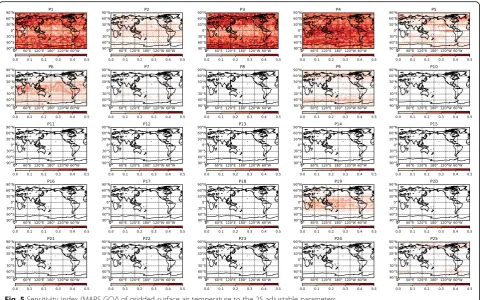
Spatial dependence of sensitivity results

Figure5shows the MARS GCV of the grid mean values

of surface air temperature to 25 adjustable parameters. This figure presents the spatial distribution of the Fig. 4Sobol’sensitivity index of global mean output variables (x-axis) to the 25 adjustable parameters (y-axis)

Table 2Output variables of LOVECLIM

No. Name Definition

1 q Specific humidity

2 ts Surface temperature

3 bm Bottom moisture

4 shf Surface sensible heat flux

5 lhf Surface latent heat flux

6 r Relative humidity

7 alb Surface albedo

8 ssr Surface solar radiation

9 tsr Top solar radiation

10 str Surface thermal radiation

11 ttr Top thermal radiation

12 evap Surface evaporation

13 pp Total precipitation

14 sp Surface pressure

15 snow Total snow fall

16 evap_land Surface evaporation over land

17 evap_sea Surface evaporation over sea

18 pp_land Total precipitation over land

19 pp_sea Total precipitation over sea

sensitivity index MARS GCV of surface air temperature, indicating the diversity of sensitivity index between land/sea surfaces and between different latitudes. Generally, there are nine parameters that are globally sensitive regarding surface temperature. Among them, P1, P3, and P4 are the most sensitive parameters for surface temperature. P1 and P3 are more sensitive in mid- and high-latitude regions, while P4 is more sensitive in tropical regions. The sensitivities of P1, P3, and P4 do not have significant land/sea differences. P2, P5, P6, P9, P19, and P25 are marginally sensitive and have some latitudinal dis-crepancies. Other parameters are nearly insensitive for every variable.

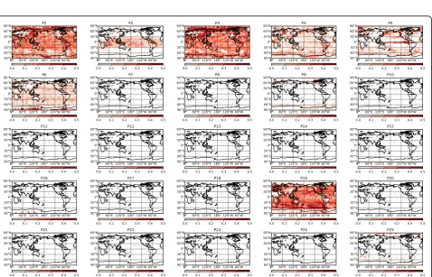
In Fig. 6, parameters P1, P3, P4, P5, and P19 are the most sensitive parameters, while P2, P6, P9, and P25 are marginally sensitive for the global grid mean values of precipitation. P5 is very sensitive in the tropical Pacific region, while P1 and P3 are not sensitive in this region. P4 has several sensitive regions west of the continents. P19, as a maximum evaporation factor over land, is sig-nificantly sensitive globally over both land and sea.

In Fig. 7, parameters P1, P3, and P19 are the parame-ters that are most sensitive to evaporation, while P2, P4, P5, P6, P9, and P25 are marginally sensitive. P2 is sensi-tive in the tropical region, and P5 is sensisensi-tive in the trop-ical Pacific.

Figures 5, 6, and7 also show the spatial distributions of the parameter sensitivities. Generally, parameters related to longwave radiation have a greater impact in mid- and high-latitude regions, while parameters related to microphysics and the land-surface evapotranspiration factor have a greater impact on low latitudes. Upon a comparison with Fig. 4, we find that the sensitivity pa-rameters are almost the same for both the grid mean values of the variables and the global mean values.

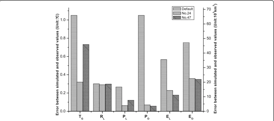
Potentials for improving climate simulations using perturbed parameters

To verify the usefulness of the sensitivity analysis, we have selected two parameters sets with better simulation results than the default parameters for the six variables involved in this paper. They are the 24th and 47th

sam-ple points of the 189 valid simulations. Figure 8

Fig. 6Sensitivity index (MARS GCV) of gridded total global precipitation to the 25 adjustable parameters

This shows that some of the errors can be greatly re-duced by tuning the most sensitive parameters, while the remained model errors can be attributed to both model structure and model input.

Conclusions

In this study, we used SA methods to identify the most sensitive parameters for surface temperature, total pre-cipitation, and total evaporation. The results of the three SA methods are consistent with each other: There are three to seven parameters that are deemed most sensi-tive in LOVECLIM depending on which climate vari-ables are evaluated. In addition, the sensitive parameters for temperature and the water cycle components are dif-ferent. Some of the sensitive parameters can affect temperature as well as climatic variable associated with the water cycle, and their effects are global. This result is very significant, as it reveals that if we would prefer to tune some of the adjustable parameters, we would need to focus on only a few of the parameters and not all of them. The spatial distribution of the parameter sensitiv-ity is different. Parameter sensitivsensitiv-ity has obvious differ-ences at different latitudes and smaller differdiffer-ences between sea and land surfaces. In general, parameters re-lated to longwave radiation have a greater impact on mid- and high latitudes, while parameters related to microphysics and the land-surface evapotranspiration have a greater impact on low latitudes. The screened pa-rameters are generally consistent with the physical inter-pretations of the model parameters. Some parameters about snow/ice albedos and ocean seem only a little sensitive.

We would like to emphasize that the 25 parameters considered here do not comprise all tunable parameters in the LOVECLIM model. Similarly, we only selected some of the important output variables in LOVECLIM for the sensitivity analysis in this study. In the future, we are going to explore the sensitivity of more parameters in more complex Earth system models and compare sen-sitivity of more output variables with advanced analysis tools. However, the results obtained here can still pro-vide a useful reference for anyone who would like to utilize a similar strategy. Furthermore, we also found that the simulation results of the climatic variables we selected from some of the sampled parameters are better than the results using the default parameters. It indicates that there is a great potential to improve climate simula-tion by optimizing the model parameters. We therefore recommend that parameters optimization should be used as one of the ways to improve the simulations of the climate system. To perform optimization in such cases, future studies must make use of more

sophisti-cated optimization tools, including the surrogate

modeling-based optimization approach, to save compu-tational resources and, therefore, feasibly achieve a multi-objective optimization strategy for the model cali-bration of complex dynamic models.

In this study, the total global runoff simulated using the default parameters is 16.28 × 103

km3(40.7%) lower

than the total global runoff obtained from the ERA-40 reanalysis data. Meanwhile, the total global precipitation and evaporation from both land and sea surfaces are lar-ger than those in the reanalysis data, implying a bias to-ward stronger global hydrological cycle compared to Fig. 8Errors between the simulated valued of global mean near-surface air temperature (TG), total global runoff over land surface (RL),

that of the real world. The biased hydrological cycle might be a possible reason for the 1 °C warmer global temperature and may lead to unknown distortions in Earth system simulations. It is almost impossible to re-duce the error only through parameter tuning if the model physics is not properly represented. If the param-eters of a physically incorrect model were forced to fit the observations, the interior processes in the model would be wrong as well, and the future climate projec-tion might be untrustworthy. The reason for the biased hydrological cycle might be due to the oversimplified land-surface hydrological processes. This leads to the problem that no matter how the parameter values are perturbed, runoff is always negatively biased. This fact suggests that although parameter calibration is some-times useful, it has limit in solving the model structure problem. Tuning the parameters, of course, does not have the ability to correct problematic or oversimplified model structures. Therefore, the model structure of LOVECLIM needs to be further improved, especially in terms of its hydrological circulation process.

Additional file

Additional file 1: Figures S1-S6.Sensitivity analysis results of current age (1951 to 2000 C.E.).Figures S7-S12.Sensitivity analysis results of pre-industrial age (1701 to 1800 C.E.). (DOCX 7939 kb)

Abbreviations

DoE:Design of experiment; EMIC: Earth system model of intermediate complexity; ESM: Earth system models; GLP: Good lattice points; LBM: Land-surface bucket model; MARS: Multivariate adaptive regression splines; NWP: Numerical weather prediction; PCE: Polynomial chaos expansion; QMC: Quasi-Monte Carlo; RF: Random forests; SA: Sensitivity analyses; SPC: Sparse polynomial chaos; UQ-PyL: Uncertainty Quantification Python Laboratory

Acknowledgements

Many thanks to Hugues Goosse in Georges Lemaître Centre for Earth and Climate Research (TECLIM), Earth and Life Institute (ELI), Université catholique de Louvain (UCL), Belgium, who helped us a lot in running the LOVECLIM model.

Authors_’contributions

QD proposed the topic, conceived, and designed the study. WG carried out the experimental study. YS analyzed the data and helped in their interpretation. JC and CX collaborated with the corresponding author in the construction of manuscript. HW carried out sensitivity analysis with the sparse PCE-based Sobol’method. All authors read and approved the final manuscript.

Authors_’information Not applicable

Funding

This work was supported by the Special Fund for Meteorological Scientific Research in Public Interest (GYHY201506002), the National Basic Research Program of China (No. 2015CB953703), the State Key Laboratory of Earth Surface Processes and Resource Ecology (No. 2017-KF-05), and the Funda-mental Research Funds for the Central Universities-Beijing Normal University Research Fund (No. 2015KJJCA04).

Availability of data and materials

The datasets generated during and/or analyzed during the current study are available from the corresponding author on reasonable request.

Competing interests

The authors declare that they have no competing interests.

Author details

1_{State Key Laboratory of Earth Surface Processes and Resource Ecology,} Faculty of Geographical Science, Beijing Normal University, Beijing 100875, China.2Institute of Land Surface System and Sustainable Development, Faculty of Geographical Science, Beijing Normal University, Beijing 100875, China.3_{Institute for Geophysics, University of Texas at Austin, 10100 Burnet} Road (R2200), Austin, TX 78758-4445, USA.

Received: 29 November 2018 Accepted: 10 June 2019

References

Allen MR, Ingram WJ (2002) Constraints on future changes in climate and the hydrologic cycle. Nature 419:224

Bastidas LA, Hogue TS, Sorooshian S, Gupta H, Shuttleworth W (2006) Parameter sensitivity analysis for different complexity land surface models using multicriteria methods. J Geophys Res Atmos 111, D20101.https://doi.org/10. 1029/2005JD006377.

Breiman L (1996) Bagging predictors. Mach Learn 24:123_–140

Breiman L (2001) Random forests. Mach Learn 45:5–32.https://doi.org/10.1023/a: 1010933404324

Brovkin V, Ganopolski A, Svirezhev Y (1997) A continuous climate-vegetation classification for use in climate-biosphere studies. Ecol Model 101:251_–261 Chahine MT (1992) The hydrological cycle and its influence on climate. Nature

359:373–380

Claussen M, Ganopolski A, Schellnhuber J, Cramer W (2000) Earth system models of intermediate complexity. Glob Chang Newsl 41:4_–6

Claussen M, Mysak L, Weaver A, Crucifix M, Fichefet T, Loutre M-F, Weber S, Alcamo J, Alexeev V, Berger A (2002) Earth system models of intermediate complexity: closing the gap in the spectrum of climate system models. Clim Dyn 18:579_–586

Collins M, Booth BB, Harris GR, Murphy JM, Sexton DM, Webb MJ (2006) Towards quantifying uncertainty in transient climate change. Clim Dyn 27:127–147 Di Z, Duan Q, Gong W, Wang C, Gan Y, Quan J, Li J, Miao C, Ye A, Tong C (2015)

Assessing WRF model parameter sensitivity: a case study with 5 day summer precipitation forecasting in the greater Beijing area. Geophys Res Lett 42: 579–587

Duan Q, Di Z, Quan J, Wang C, Gong W, Gan Y, Ye A, Miao C, Miao S, Liang X (2017) Automatic model calibration: a new way to improve numerical weather forecasting. Bull Am Meteorol Soc 98:959–970

Eby M, Weaver AJ, Alexander K, Zickfeld K, Abe-Ouchi A, Cimatoribus A, Crespin E, Drijfhout S, Edwards N, Eliseev A (2013) Historical and idealized climate model experiments: an intercomparison of Earth system models of intermediate complexity. Clim Past 9:1111–1140

Edwards NR, Marsh R (2005) Uncertainties due to transport-parameter sensitivity in an efficient 3-D Ocean-climate model. Clim Dyn 24:415–433

Efron B (1979) Bootstrap methods: another look at the jackknife. Ann Stat 7:1_–26. Eyring V et al (2016) ESMValTool (v1.0)—a community diagnostic and

performance metrics tool for routine evaluation of Earth system models in CMIP. Geosci Model Dev 9:1747–1802. https://doi.org/10.5194/gmd-9-1747-2016

Fanning AF, Weaver AJ (1997) A horizontal resolution and parameter sensitivity study of heat transport in an idealized coupled climate model. J Clim 10: 2469–2478

Friedman JH (1991) Multivariate adaptive regression splines. Ann Stat 19:1_–67 Gan Y, Duan Q, Gong W, Tong C, Sun Y, Chu W, Ye A, Miao C, Di Z (2014) A

comprehensive evaluation of various sensitivity analysis methods: a case study with a hydrological model. Environ Model Softw 51:269–285 Gent PR, Danabasoglu G, Donner LJ, Holland MM, Hunke EC, Jayne SR, Lawrence

DM, Neale RB, Rasch PJ, Vertenstein M (2011) The community climate system model version 4. J Clim 24:4973–4991

Gong W, Duan Q, Li J, Wang C, Di Z, Dai Y, Ye A, Miao C (2015) Multi-objective parameter optimization of common land model using adaptive surrogate modeling. Hydrol Earth Syst Sci 19:2409–2425

Gong W, Duan Q, Li J, Wang C, Di Z, Ye A, Miao C, Dai Y (2016a) An intercomparison of sampling methods for uncertainty quantification of environmental dynamic models. J Environ Inf 28:11–24

Gong W, Duan Q, Li J, Wang C, Di Z, Ye A, Miao C, Dai Y (2016b) Multiobjective adaptive surrogate modeling-based optimization for parameter estimation of large, complex geophysical models. Water Resour Res 52:1984–2008 Goosse H, Brovkin V, Fichefet T, Haarsma R, Huybrechts P, Jongma J, Mouchet A,

Selten F, Barriat PY, Campin JM, Deleersnijder E, Driesschaert E, Goelzer H, Janssens I, Loutre MF, Maqueda MAM, Opsteegh T, Mathieu PP, Munhoven G, Pettersson EJ, Renssen H, Roche DM, Schaeffer M, Tartinville B, Timmermann A, Weber SL (2010) Description of the Earth system model of intermediate complexity LOVECLIM version 1.2. Geosci Model Dev 3:603–633.

https://doi.org/10.5194/gmd-3-603-2010

Goosse H, Driesschaert E, Fichefet T, Loutre M-F (2007) Information on the early Holocene climate constrains the summer sea ice projections for the 21st century. Clim Past 3:683–692

Goosse H, Fichefet T (1999) Importance of ice-ocean interactions for the global ocean circulation: a model study. J Geophys Res Oceans 104:23337–23355 Goosse H, Selten F, Haarsma R, Opsteegh J (2001) Decadal variability in high

northern latitudes as simulated by an intermediate-complexity climate model. Ann Glaciol 33:525–532

Goosse H, Selten F, Haarsma R, Opsteegh J (2002) A mechanism of decadal variability of the sea-ice volume in the northern hemisphere. Clim Dyn 19: 61–83

Gupta HV, Razavi S (2018) Revisiting the basis of sensitivity analysis for dynamical earth system models. Water Resour Res.https://doi.org/10.1029/

2018WR022668

Gutiérrez ÁG, Schnabel S, Contador JFL (2009) Using and comparing two nonparametric methods (CART and MARS) to model the potential distribution of gullies. Ecol Model 220:3630–3637

Hansen J, Sato M, Ruedy R, Lo K, Lea DW, Medina-Elizade M (2006) Global temperature change. Proc Natl Acad Sci U S A 103:14288–14293.https://doi. org/10.1073/pnas.0606291103

Hlawka E (1962) Zur angenäherten berechnung mehrfacher integrale. Monatshefte für Mathematik 66:140–151

Hourdin F, Mauritsen T, Gettelman A, Golaz J-C, Balaji V, Duan Q, Folini D, Ji D, Klocke D, Qian Y (2017) The art and science of climate model tuning. Bull Am Meteorol Soc 98:589–602

Huybrechts P (2002) Sea-level changes at the LGM from ice-dynamic reconstructions of the Greenland and Antarctic ice sheets during the glacial cycles. Quat Sci Rev 21:203–231

IPCC (2007) Climate Change 2007: The Scientific Basis. Contribution of Working Group I to the Fourth Assessment Report of the Inter-governmental Panel on Climate Change. Cambridge University Press, Cambridge

IPCC (2013) Climate Change 2013: The Scientific Basis. Contribution of Working Group I to the Fourth Assessment Report of the Inter-governmental Panel on Climate Change. Cambridge University Press, Cambridge

Johannesson G, Lucas D, Qian Y, Swile L, Wildey TM (2014) Sensitivity of precipitation to parameter values in the Community Atmosphere Model Version 5. Sandia report SAND2014–0829 Sandia National Laboratories, Albuquerque

Jones JAA (2014) Global hydrology: processes, resources and environmental management. Routledge, London

Korobov N (1959a) The approximate computation of multiple integrals. Dokl Akad Nauk SSSR 6:1207–1210

Korobov N (1959b) Computation of multiple integrals by the method of optimal coefficients. Vestn Mosk Univ, Ser Mat, Mekh, Astron, Fiz, Khim 4:19_–25 Korobov N (1960) Properties and calculation of optimal coefficients. Dokl Akad

Nauk SSSR 132:1009–1012

Levy S, Steinberg DM (2010) Computer experiments: a review. AStA Adv Stat Anal 94:311_–324

Liu Y, Gupta HV, Sorooshian S, Bastidas LA, Shuttleworth WJ (2004) Exploring parameter sensitivities of the land surface using a locally coupled land-atmosphere model. J Geophys Res: Atmos 109, D21101.https://doi.org/ 10.1029/2004JD004730.

Loutre MF, Mouchet A, Fichefet T, Goosse H, Goelzer H, Huybrechts P (2011) Evaluating climate model performance with various parameter sets using

observations over the recent past. Clim Past 7:511–526.https://doi.org/ 10.5194/cp-7-511-2011

Mauritsen T, Stevens B, Roeckner E, Crueger T, Esch M, Giorgetta M, Haak H, Jungclaus J, Klocke D, Matei D, Mikolajewicz U, Notz D, Pincus R, Schmidt H, Tomassini L (2012) Tuning the climate of a global model. J Adv Model Earth Syst 4.https://doi.org/10.1029/2012ms000154

Mouchet A, François L (1996) Sensitivity of a global oceanic carbon cycle model to the circulation and to the fate of organic matter: preliminary results. Phys Chem Earth 21:511–516

Murphy JM, Sexton DM, Barnett DN, Jones GS, Webb MJ, Collins M, Stainforth DA (2004) Quantification of modelling uncertainties in a large ensemble of climate change simulations. Nature 430:768–772

Neelin JD, Bracco A, Luo H, McWilliams JC, Meyerson JE (2010) Considerations for parameter optimization and sensitivity in climate models. Proc Natl Acad Sci 107:21349–21354

Opsteegh J, Haarsma R, Selten F, Kattenberg A (1998) ECBILT: a dynamic alternative to mixed boundary conditions in ocean models. Tellus A 50: 348_–367

Pati YC, Rezaiifar R, Krishnaprasad PS (1993. IEEE) Orthogonal matching pursuit: recursive function approximation with applications to wavelet

decomposition. In: Proceedings of 27th Asilomar conference on signals, systems and computers, pp 40–44

Petoukhov V, Claussen M, Berger A, Crucifix M, Eby M, Eliseev A, Fichefet T, Ganopolski A, Goosse H, Kamenkovich I (2005) EMIC Intercomparison project (EMIP–CO2): comparative analysis of EMIC simulations of climate, and of equilibrium and transient responses to atmospheric CO2 doubling. Clim Dyn 25:363–385

Quan J, Di Z, Duan Q, Gong W, Wang C, Gan Y, Ye A, Miao C (2016) An evaluation of parametric sensitivities of different meteorological variables simulated by the WRF model. Q J R Meteorol Soc 142:2925–2934 Ratto M, Castelletti A, Pagano A (2012) Emulation techniques for the reduction

and sensitivity analysis of complex environmental models

Renssen H, Brovkin V, Fichefet T, Goosse H (2003) Holocene climate instability during the termination of the African humid period. Geophys Res Lett 30: 1184.https://doi.org/10.1029/2002GL016636.

Renssen H, Goosse H, Fichefet T, Brovkin V, Driesschaert E, Wolk F (2005) Simulating the Holocene climate evolution at northern high latitudes using a coupled atmosphere-sea ice-ocean-vegetation model. Clim Dyn 24:23–43 Ricciuto D, Sargsyan K, Thornton P (2018) The impact of parametric uncertainties

on biogeochemistry in the E3SM land model. J Adv Model Earth Syst 10: 297_–319.https://doi.org/10.1002/2017ms000962

Sanderson BM, Piani C, Ingram W, Stone D, Allen M (2008) Towards constraining climate sensitivity by linear analysis of feedback patterns in thousands of perturbed-physics GCM simulations. Clim Dyn 30:175_–190 Santanello JA Jr, Peters-Lidard CD, Kumar SV (2011) Diagnosing the sensitivity of

local land–atmosphere coupling via the soil moisture–boundary layer interaction. J Hydrometeorol 12:766_–786

Sarrazin F, Pianosi F, Wagener T (2016) Global sensitivity analysis of

environmental models: convergence and validation. Environ Model Softw 79: 135–152.https://doi.org/10.1016/j.envsoft.2016.02.005

Shahsavani D, Grimvall A (2011) Variance-based sensitivity analysis of model outputs using surrogate models. Environ Model Softw 26:723_–730 Shahsavani D, Tarantola S, Ratto M (2010) Evaluation of MARS modeling

technique for sensitivity analysis of model output. Procedia Soc Behav Sci 2: 7737_–7738

Sobol_’IM (1993) Sensitivity estimates for nonlinear mathematical models. Math Modelling Comput Experiments 1:407–414

Steinberg D, Colla P, Martin K (1999). MARS User Guide. Salford Systems, San Diego Sudret B (2008) Global sensitivity analysis using polynomial chaos expansions.

Reliab Eng Syst Saf 93:964–979.https://doi.org/10.1016/i.ress.2007.04.002

Tan J, Cui Y, Luo Y (2017) Assessment of uncertainty and sensitivity analyses for ORYZA model under different ranges of parameter variation. Eur J Agron 91:54_–62 Tang T, Reed P, Wagener T, Van Werkhoven K (2006) Comparing sensitivity

analysis methods to advance lumped watershed model identification and evaluation. Hydrol Earth Syst Sci Discuss 3:3333_–3395

Tebaldi C, Knutti R (2007) The use of the multi-model ensemble in probabilistic climate projections. Philos Trans Royal Soc London A: Mathematical, Physical and Engineering Sciences 365:2053–2075

Wang C, Duan Q, Tong CH, Di Z, Gong W (2016) A GUI platform for uncertainty quantification of complex dynamical models. Environ Model Softw 76:1_–12 Williamson D, Goldstein M, Allison L, Blaker A, Challenor P, Jackson L, Yamazaki K

(2013) History matching for exploring and reducing climate model parameter space using observations and a large perturbed physics ensemble. Clim Dyn 41:1703_–1729

Xiong S-y, X-m Z, J-b L, Wu Z-h (2010) Numerical simulation on the sensitivity of a heavy rain case to the random disturbances of land surface parameters. Torrential Rain Disasters 29:117–121

Zadeh FK, Nossent J, Sarrazin F, Pianosi F, van Griensven A, Wagener T, Bauwens W (2017) Comparison of variance-based and moment-independent global sensitivity analysis approaches by application to the SWAT model. Environ Model Softw 91:210–222.https://doi.org/10.1016/j.envsoft.2017.02.001 Publisher’s Note