O R I G I N A L A R T I C L E
Open Access
Intergenerational mobility in Korea
Soobin Kim
Correspondence: [email protected]
College of Education, Michigan State University, 620 Farm Lane, Room 516, Erickson Hall, East Lansing, MI 48824-1038, USA
Abstract
This study investigates intergenerational earnings mobility in Korea for sons born between 1958 and 1973 and compares Korea’s mobility to that of other nations. It uses data from the Korea Labor and Income Panel Study and the Household Income and Expenditure Survey conducted by the Korean National Statistics Bureau. Since no single Korean dataset includes information on both sons’ and their fathers’ adult earnings, this study follows the two-sample approach previously applied in Korea by Ueda (J Asian Econ 1–22, 2013), whose estimated intergenerational earnings elasticity is 0.22, and extends the analysis by using fathers’ earnings from a more approximal cohort. The estimate of around 0.4 is similar to estimates for some already developed countries and smaller than typical estimates for recently developing countries.
JEL classification: J62, J31
Keywords: Intergenerational earnings mobility, Generated regressor, Two-sample estimation
1 Introduction
Intergenerational mobility refers to the persistence between parents’ and children’s out-comes. If parents’ earnings do not impact much on their offspring’s earnings, the degree of intergenerational earnings mobility is high, and it could be that relative economic disadvantages in the early years will persist to a lower extent in adulthood. That is, intergenerational earnings mobility explores the characteristics of inequality in economic opportunity as well. For a survey of relevant literature, see Solon (1999) and Black and Devereux (2010).
Some features of Korea make it an interesting case for the study of intergenerational mobility. First, Korea experienced rapid and extensive economic growth in the past half century when the real GDP per capita increased 15-fold. At the same time, inequality in labor earnings steadily decreased from the 1970s to the 1990s. The extent to which these changes in labor market conditions is related to the high degree of intergenerational mobility is an interesting question. Second, the Korean education system is very compet-itive due to the strong desire of Koreans for education, and Korea went through a great expansion in education in the last few decades. At the same time, education has been viewed as a vehicle to the next highest level of schooling and a means of obtaining higher socio-economic status (Korea 1991). Thus, whether the intergenerational mobility varies with parental education is another relevant question to answer.
Because of a lack of longitudinal data spanning two generations, only a limited number of studies on intergenerational earnings mobility in Korea have been done. Recent studies in Korea by Kim (2009) and Choi and Hong (2011) employed co-residing father-son pairs
in the initial round of panel data. However, as noted by Solon (2002), this sample may dis-play a different intergenerational association than would a more representative sample.1 Moreover, as in most other empirical studies, they estimated intergenerational earnings elasticities using short-run proxies for permanent earnings, which may generate down-ward biases in estimates.2An important exception avoiding this difficulty is Ueda (2013) who utilized a two-sample method to impute fathers’ permanent earnings and showed relatively higher estimated intergenerational earnings mobility in Korea.
This study estimates intergenerational earnings mobility in Korea following the method presented in Ueda (2013) and extends empirical analysis in two dimensions. First, I use an additional national representative sample to better approximate the actual fathers’ birth cohorts so that fathers’ missing permanent earnings are more accurately imputed. I also carefully choose age ranges for each generation to minimize life-cycle bias that stems from using current earnings for lifetime earnings.3Second, I compare the intergenera-tional mobility of Korea with that of 13 other countries that come from the two-sample method. The intergenerational elasticity estimate of around 0.4 in Korea is similar to that in already developed countries and relatively smaller than recently developed or developing countries.
The remainder of this study is organized as follows: Section 2 describes the method-ology employed in early literature. Section 3 discusses the data. Section 4 presents the empirical results. Section 5 concludes with remarks.
2 Literature review and method
In this section, I provide a skeletal derivation of the intergenerational mobility developed in Solon (1992) and Björklund and Jäntti (1997). The basic empirical approach in inter-generational mobility literature is to estimate earnings elasticity, which is to estimateρ1 in the following equation.
yi=ρ0+ρ1xi+i (1)
whereyiis the log of the permanent component of the son’s earnings in familyi,xiis the
log of the permanent component of the father’s earnings in familyi, andi is a random
disturbance uncorrelated withxi. Ifyiandxiare observed directly from a random sample,
one can estimateρ1in Eq. (1) by applying least squares regression. Here the parameterρ1 is the intergenerational earnings elasticity and (1−ρ1) can be interpreted as a measure of intergenerational mobility. Therefore, by comparingρˆ1of each country, comparisons of intergenerational mobility across countries are possible; the higherρˆ1is, the less mobile the society is.4
However, in most studies, available measures of the earnings variable are current earnings in repeated cross-section samples or in longitudinal samples, and in practice, researchers have used short-run proxies ofyitfor long-run economic status variables ofyi
in timet,
yit=λtyi+h(Ageit)+νit (2)
where λt is the association between current and lifetime earnings at time t, which is
allowed to vary over the life cycle, andνit, the measurement error inyitas a proxy foryi,
is assumed to be uncorrelated withyiandi.h(Ageit)is an arbitrary function of a son’s
If one has an appropriate measure of a father’s long-run earnings but is forced to use current earnings as a proxy for the son’s long-run earnings, plugging Eq. (1) into Eq. (2) yields
yit=λtρ0+λtρ1xi+h
Ageit+ηit (3)
whereηit is equal toλti+νit. In addition to the measurement error in lifetime
earn-ings, Haider and Solon (2006) and Grawe (2006) presented empirical evidence of another source of inconsistency that short-run earnings deviate from long-run earnings over the life cycle: The probability limit of the least squares estimator of the coefficient ofxiis equal
toλtρ1. Haider and Solon (2006) suggested the age ranges be used for both father and son around their mid-careers, which would more accurately represent lifetime earnings.5
Another estimation problem exists when a single dataset containing earnings data for pairs of fathers and sons in a long-time series is unavailable. Björklund and Jäntti (1997) proposed a two-sample method to impute fathers’ missing earnings from an auxiliary sample of a father’s generation on the basis of a son’s report on a father, such as educa-tion, industry, and occupation.6Letzidenote a set of fathers’ socio-demographic variables
such as education and occupation and assume that the permanent component of fathers’ earnings is generated by the following relationship:
xi=ziφ+ξi (4)
whereziis orthogonal toξiby linear projection. From Eq. (4), fathers’ long-run economic
status variables are generated,xˆi=ziφˆ, with age controls in the potential fathers’ sample.7
Rewrite Eq. (1) asyi=ρ0+ρ1xˆi+i+ρ1(xi− ˆxi)and plug into Eq. (2) gives
yit=λtρ0+λtρ1xˆi+h(Ageit)+ωit (5)
whereωitis equal toλti+νit+λtρ1(xi− ˆxi). Under regularity conditions described in
the Appendix, the probability limit of the least squares estimator of the coefficient ofxiis
equal to
plimn→∞ρˆ1= λtρ1
Var(xi)+Cov(xi,νit)
Var(xi)
(6)
which reduces toλtρ1if Cov(xi,νit) = 0. (The proof can be reviewed in the Appendix).
However, the consistency still depends onλt even with the generated regressor, and it
calls for researcher caution in choosing the appropriate age range as Haider and Solon (2006) proposed. Nybom and Stuhler (2016) used long series of Swedish income data that contain nearly complete income histories of both fathers and sons and verified Haider and Solon’s implications that the life-cycle bias is smallest when incomes are observed around midlife and that the life-cycle bias cannot be eliminated at other ages.8Finally, ordinary least squares regression is applied to Eq. (5) to estimateρ1.9
were at a specific age as reported in the first dataset. Thenρ1 can be estimated from Eq. (5) with predicted fathers’ earnings,xˆi, in lieu of fathers’ permanent earnings,xi.
Similar to many other countries, Korea does not have a sufficiently long intergen-erational panel dataset where explicit information of father-son pairs’ economic status variables are observed. Several studies in Korea were done by employing the Korean Labor and Income Panel Study (KLIPS). Using KLIPS, Kim (2009) and Choi and Hong (2011) focused on father-son pairs who co-resided in 1998 and restricted sons who in subsequent years moved into a non-member household (for instance, through marrying). This homo-geneous sample of co-resident father-son pairs is an endogenously selected sample and would demonstrate an intergenerational transmission of earnings different from the pop-ulation. They averaged available earnings to overcome attenuation bias because current earnings are proxied for permanent earnings. However, including younger sons—around 30—and older fathers—in the late 50s—tends to lower estimates due to life-cycle bias. For monthly earnings, coefficients are 0.141 (0.042) and 0.349 (0.096) when the father’s education is instrumented for the father’s earnings.
Ueda (2013) also used KLIPS to estimate intergenerational mobility in Korea and employed a two-sample method to impute actual fathers’ permanent earnings using sons’ recollections of their fathers’ educational levels and occupations when they were 14. Among working men with positive wages aged 25–54 for fathers and 30–39 for sons, Ueda restricted the sons’ sample to 2006 and pooled annual earnings for the potential fathers’ sample observed over the period 2003–2006. The coefficient is 0.223 (0.072), but Ueda imputed a too-recent earnings function instead of choosing the fathers’ sample in actual calendar time.
3 Data
KLIPS contains sons’ earnings and their recollections of fathers when they were 14 and is the first Korean longitudinal survey on the labor market and income activities of house-holds and individuals, collected from 1998 to 2008. During the first wave in 1998, a representative sample of 5000 households and their members (15 and over), covering more than 13,000 individuals, was interviewed using the sampling frame from the census, and they became the original panel of households and household members.
In addition, Household Income and Expenditure Survey (HIES) is repeated cross-section survey data that are the only publicly available data at an individual level with economic status variables such as labor earnings, family income information of each household, and socio-demographic characteristics. Survey data are available since 1982; however, education information was added to the survey since 1985. HIES, as in KLIPS, used the sampling frame of the census, which supports the argument that both datasets are representative samples of the Korean labor market.
suited to measure mobility based on an individual’s merit than do other economic status variables.11
KLIPS and HIES have recorded education, occupation, and industry in different cat-egories. Especially occupation and industry variables are recorded with three digits in KLIPS, but in one digit and two digits in HIES, respectively. Since the categories used for industry and occupation in KLIPS are finer than those used in HIES, those variables are matched according to the HIES category. After recoding categories to have a homo-geneous classification across samples, seven different levels of education, nine industry groups, and seven occupational groups are available to predict fathers’ missing earnings. The number of predictors for fathers’ missing earnings as well as the number of groups of each variable are relatively richer than in previous studies in other countries.12
In the analysis, I use two waves of KLIPS for the sons’ sample and both KLIPS and HIES for the potential fathers’ sample. When replicating Ueda’s empirical results, I use KLIPS in 2006 for the sons’ sample and KLIPS in 2003 for the potential fathers’ sample. Since the age gap between sons in KLIPS in 2006 and potential fathers in KLIPS in 2003 is three, to use more approximal cohorts of actual fathers, I retrieve the sons’ sample from KLIPS in 2008 and the potential fathers’ sample from HIES in 1985. These two samples are 23 years apart which thus enables matching of the father’s generation more closely to actual fathers than does using 2003 for the potential fathers’ sample.13
Preferred age range for both generations is between 35 and 50 as the errors-in-variables bias in sons’ earnings stays small, modifying the results from Haider and Solon (2006) given that Korean male workers generally enter the labor market about 3–5 years later than in the USA due to mandatory military service obligations.14
Both KLIPS in 2008 and HIES in 1985 are restricted to working men aged between 35 and 50 with positive wages, which leaves 1700 observations in KLIPS and 1780 in HIES.15 Especially in HIES, the fathers’ sample was further restricted to those with a positive number of children aged 6–19 in 1985. Fathers or sons who lived in foreign countries when their sons were 14 are excluded. Narrowing the sample to those with all education, industry, and occupation variables recorded, the number of observation drops to 1666 in KLIPS and 1577 in HIES. Descriptive statistics of variables used for the main sample and the supplemental sample are summarized in Table 1.
4 Empirical results
Table 1Descriptive statistics
Actual fathers Potential fathers described by sons
Sons in HIES
Mean age 41 41
Education
None 6.9 1.7 0.2
Elementary 26.1 15.4 1.8
Middle 20.8 23.7 4.1
High 29.2 34.8 30.6
Community college (2 years) 2.0 2.4 18.2 University (4 years) 13.7 20.4 34.3 Graduate school 1.4 1.7 10.8 Occupation
Professional, technical, managerial 12.7 8.1 36.5 High-rank government officer, entrepreneur 2.6 0.7 2.6 Administrative worker 16.7 24.9 19.2 Office worker 5.2 7.7 3.7 Service worker 3.2 5.3 3.5 Production worker 37.4 51.1 33.3 Agriculture, fishing, forestry 22.3 2.2 1.2 Industry
Agriculture, fishing, forestry 12.1 2.0 0.6
Mining 2.4 1.5 0.0
Manufacturing 18.2 30.3 28.6 Utilities 0.2 1.1 1.4 Construction 19.6 18.0 12.6 Wholesale and retail trade 10.3 8.8 11.6 Communication, transportation 8.9 12.3 7.7 Banking, business service 5.0 4.1 17.8 Public administration, education 23.4 22.0 19.8
Note: Age of father-son sample is restricted to 35–50
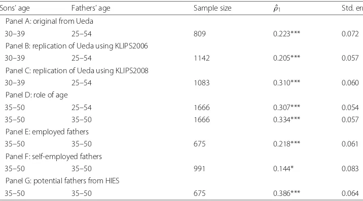
Table 2Intergenerational earnings elasticity
Sons’ age Fathers’ age Sample size ρˆ1 Std. err
Panel A: original from Ueda
30–39 25–54 809 0.223*** 0.072 Panel B: replication of Ueda using KLIPS2006
30–39 25–54 1142 0.205*** 0.057 Panel C: replication of Ueda using KLIPS2008
30–39 25–54 1083 0.310*** 0.060 Panel D: role of age
35–50 25–54 1666 0.307*** 0.054 35–50 35–50 1666 0.334*** 0.057 Panel E: employed fathers
35–50 35–50 675 0.218*** 0.061 Panel F: self-employed fathers
35–50 35–50 991 0.144* 0.083 Panel G: potential fathers from HIES
35–50 35–50 675 0.386*** 0.064
Notes: Sons’ information is retrieved from KLIPS 2006 for panels A–B and from KLIPS 2008 for panels C–G. Potential fathers’ information is retrieved from KLIPS 2003 for panels A–F and from HIES 1985 for panel G. Bootstrapped standard errors are in parentheses
is 0.205 with a bootstrapped standard error of 0.057, which is similar to Ueda’s base-line estimate of 0.223. Ueda used education and occupation to predict fathers’ missing earnings, and when I use those two variables as predictors, the estimate is 0.244 (0.094). When the later round in 2008 is used for the sons’ sample, the estimate is 0.310 (0.060) which suggests that detailed matching of potential fathers with actual fathers could be important.
Restricting to the preferred age range of 35–50 for both generations, the estimate in panel D increases to 0.334 (0.057), partly due to excluding young fathers. Results are con-sistent with previous studies on life-cycle bias; inclusion of younger sons or older fathers lowers estimates. That is, the correlation between a father’s age (son’s age) at measure-ment and the size ofρˆ1is negative (positive). The next two panels examine whether the elasticity is different with respect to the father’s self-employment status. Nine hundred and ninety-one out of 1666 sons have self-employed fathers when they were 14, and the estimates are 0.144 (0.083) for sons with self-employed fathers and 0.218 (0.061) for sons with employed fathers, which frees concern that the self-employment status of fathers might significantly affect the estimates.
Approximating pseudo-fathers’ earnings with recent cohorts, however, implicitly assumes that potential fathers’ characteristics in 2003 are close to those for actual fathers, and uses information from the younger-father generation. In other words, if the aver-age aver-age gap between fathers and sons is 30, then fathers’ actual aver-ages in 2003, whose sons are aged 30–39 in 2008, are 55–64 instead of 25–54. Moreover, occupation, industry, and education distribution in 2003, used for potential fathers’ characteristics, are more similar to those for sons in 2008 than to those for actual fathers. Thus, results of this approach are vulnerable if one supposes significant changes occurred in the wage struc-ture in recent decades. To retrieve potential fathers’ information from a more approximal cohort of actual fathers, I use HIES and generate pseudo-fathers’ earnings based on sons’ recollections on fathers’ characteristics.
4.1 The role of HIES
By retrieving potential fathers’ information from HIES in 1985, the father-son age gap becomes more realistic and the distribution of earnings predictors including education, occupation, and industry becomes closer to those of actual fathers remembered by sons than to those of potential fathers in KLIPS 2003.
Age ranges for both generations are restricted to 35–50 as it best reflects the fea-ture of the Korean labor market that mandatory military service generally delays men from joining it. Moreover, the preferred age range better represents mid-career earnings, and this specification with three earnings predictors for fathers is served as the baseline model.18 By excluding younger sons in their later 20s and early 30s and older fathers above 50, the estimate increases to 0.386 (0.064) in panel G in Table 2.19
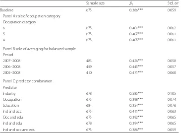
Table 3Sensitivity of intergenerational earnings elasticity
Sample size ρˆ1 Std. err
Baseline 675 0.386*** 0.059 Panel A: role of occupation category
Occupation category
6 675 0.401*** 0.062
5 675 0.407*** 0.061
4 675 0.405*** 0.061
Panel B: role of averaging for balanced sample Period
2007–2008 483 0.426*** 0.058 2006–2008 459 0.445*** 0.057 2005–2008 410 0.471*** 0.060 Panel C: predictor combination
Predictor
Industry 678 0.585*** 0.105 Occupation 675 0.398*** 0.074 Education 684 0.354*** 0.076 Ind and occ 675 0.411*** 0.063 Occ and edu 675 0.392*** 0.065 Ind and edu 678 0.394*** 0.065 Ind and occ and edu 675 0.386*** 0.059
Notes: The baseline model uses industry, occupation, and education as predictors, and the age of the father-son sample is restricted to 35–50. Seven groups of occupation category are used, and standard errors are bootstrapped
***significant at the 1% level
0.401 to 0.407 when the number of occupation categories is changed from 6 to 4, which indicates that the estimates are robust to occupation specifications. Thus, a different occupation category distribution has negligible impact on estimates.
The age range of 35–50 is chosen to haveλtclose to 1 so that the measurement error
is close to the classical errors-in-variables. Many studies using current earnings to proxy for permanent earnings averaged earnings over years to deal with the measurement error following Solon (1992). Estimates of intergenerational earnings elasticity become larger as fathers’ earnings are averaged over more years. As potential fathers are taken from HIES in 1985 and HIES is repeated cross-section data, calculating missing father’s average earnings is challenging. In addition, Nybom and Stuhler (2016) provided evidence that changing the age span for sons has more impact on life-cycle bias than changing that of fathers. Thus, sons’ earnings are averaged over years, and the results in panel B show that the estimates increase as earnings are averaged over more years.
In the base model, all three earnings predictors are used. If one changes the combi-nation of earnings predictors and uses a subset of predictors, sample size increases by only nine, which frees the concern of having a smaller sample size in exchange for hav-ing more predictors. Results in panel C indicate that the estimates change from 0.35 to 0.59, suggesting that researchers should pay attention when they choose appropriate pre-dictors. Equation (6) implies that the estimator with a generated regressor is inconsistent if father’s earnings predictors are correlated with son’s earnings (Cov(xi,νit) = 0). For
father’s industry or occupation are correlated with son’s earnings is less clear and so is the direction of bias. In addition, first-stage results from Table 4 show that the indus-try variable explains relatively less variations in earnings than occupation or education does, which could result in a higherρˆ1of 0.59. On the other hand, all other estimates that used father’s education as a predictor are close to 0.39. For comparison, majority of other countries’ studies on intergenerational elasticity with two-sample estimation, documented in Table 5, did not use an industry variable to predict fathers’ earnings. How-ever, it is not clear in which direction the estimate would move if an industry variable is included.20
4.2 International comparison
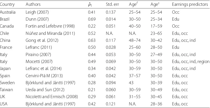
Table 5 summarizes the evidence of intergenerational mobility from 13 other countries that come from two-sample estimation. For comparability with the Korea results, the table focuses on the earnings elasticity estimates of father-son pairs and lists the age ranges and sets of predictors used to generate fathers’ earnings. While Nybom and Stuhler (2016) pointed out that the bias in elasticity estimates can differ across countries and cohort even if earnings are measured at the same age, we might expect similarities in its broad patterns. The intergenerational elasticity estimate around 0.4 in Korea is similar to that of already developed countries and relatively smaller than recently developed or devel-oping countries. That is, the mobility in Korea is relatively higher than other develdevel-oping countries (e.g., 0.69 in Brazil and 0.52 in Chile).21
Some studies, for instance Piraino (2007) in Italy, investigated the channels in the transmission of economic status and found parental education’s contribution to the inter-generational mobility. Korea went through a great expansion in education in the last few decades, and the parent-child schooling correlation among 20–69 sons in 2008 is only 0.333, one of the lowest values according to Hertz et al. (2008).22In particular, approxi-mately 60% of sons in 2008 are educated beyond high schools, whereas about 50% of their fathers have education equal or less than middle school. At the same time, there is a dif-ferential probability of attaining post-secondary education degree by father’s status. For example, the probability of attaining college or advanced degree is 32 percentage points higher for sons whose fathers are educated more than middle school. As the wage gap between sons with a college or advanced degree and those with no education beyond high school is 100% in 2008, I estimate the role of education as a channel of intergenerational transmission by adding the son’s education dummy variables to Eq. (5). The resulting
ˆ
ρ1 = 0.196 suggests that education explains 49% of the observed persistence, which is
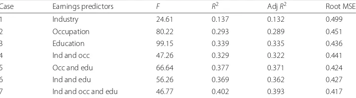
Table 4Choice of father’s earnings predictors
Case Earnings predictors F R2 AdjR2 Root MSE 1 Industry 24.61 0.137 0.132 0.499 2 Occupation 80.22 0.293 0.289 0.451 3 Education 99.15 0.339 0.335 0.436 4 Ind and occ 47.26 0.329 0.322 0.441 5 Occ and edu 66.64 0.377 0.371 0.424 6 Ind and edu 56.26 0.369 0.362 0.427 7 Ind and occ and edu 46.77 0.402 0.393 0.417
Table 5Comparable intergenerational earnings elasticity with two-sample estimation
Country Authors ρˆ1 Std. err Agef Ages Earnings predictors
Australia Leigh (2007) 0.41 0.137 25–54 25–54 Occ Brazil Dunn (2007) 0.69 0.014 30–50 25–34 Edu Canada Fortin and Lefebvre (1998) 0.22 0.051 40–50 17–59 Occ Chile Núñez and Miranda (2011) 0.52 N.A. N.A. 23–65 Edu, occ China Gong et al. (2012) 0.63 0.117 48–74 30–42 Edu, occ, ind France Lefranc (2011) 0.50 0.028 25–60 28–50 Edu Italy Piraino (2007) 0.44 0.053 30–50 27–49 Edu, occ, ind Italy Mocetti (2007) 0.49 0.069 30–50 30–50 Edu, occ, ind, region Japan Lefranc et al. (2014) 0.34 0.042 30–59 30–50 Edu, occ, ind Spain Cervini-Plá M (2013) 0.40 0.042 37–57 30–50 Edu, occ Sweden Björklund and Jäntti (1997) 0.28 0.094 43 30–39 Edu, occ Taiwan Ueda and Sun (2012) 0.21 0.060 30–59 30–49 Edu, occ UK Nicoletti and Ermisch (2008) 0.29 0.061 31–55 30–45 Edu, occ USA Björklund and Jäntti (1997) 0.42 0.121 N.A. 28–36 Edu, occ
Notes: Leigh (2007) used predicted hourly wage for a 40-year-old, and the estimates in the table show results with the 1987 sample. When the 2004 sample is used, the estimate is 0.18 with standard errors of 0.043. Fortin and Lefebvre (1998) assumed a 25–35-year difference between father and son. Björklund and Jäntti (1997) used the mean age of 43
N.A.not applicable
similar to the previous findings in the USA (Bowles and Gintis 2002; Blanden et al. 2014). Additional analysis shows that intergenerational mobility differs with respect to father’s education. In particular, sons whose fathers have an education equal or less than middle school have the highest intergenerational elasticity estimate of 0.415. On the contrary, the elasticity estimate for sons whose fathers have a high school degree is 0.252. Finally, the estimate for sons whose fathers have a college or more advanced degree is 0.193, which indicates the highest intergenerational earnings mobility. The extent to which the dif-ferential intergenerational mobility by the father’s education translates into the earnings inequality is important for future research.
5 Remarks
This study examines intergenerational earnings mobility in Korea with the two-sample estimation method to generate the father’s missing permanent earnings by combining a panel dataset, which includes the son’s earnings and recollection information on the father’s socio-demographic characteristics, and a cross-section dataset, which contains earnings and socio-demographic information of potential fathers. Results indicate that the measurement error in sons’ current earnings as a proxy for permanent earnings is a source of inconsistency even when fathers’ earnings are generated. Thus, the working father-son sample is restricted to age 35–50 to be least affected by the life-cycle bias, and the elasticity estimate is around 0.4. Estimated intergenerational earnings elasticity is similar to estimates for some already developed countries and smaller than typical estimates for recently developing countries.
inaccurate period of observation for the potential fathers’ sample was used for impu-tation.23 Thus, this study contributes to more acute estimation of mobility, with two representative samples aiming to match pairs correctly by choosing the right age range for both generations, which better represents permanent earnings.
Perhaps one of the most important remaining issues to deal with is the life-cycle bias in Korea. As Nybom and Stuhler (2016) suggested, life-cycle bias will differ quantitatively across countries and cohorts, and small age deviations can cause notable changes in elas-ticity estimates, which appears to be relevant in the Korean context. For example, male workers in Korea generally have to serve in the army from their late teens, which on aver-age delays labor market participation timing by 3 to 5 years compared to the USA. Since data access to individual earnings histories for multiple generations is limited in Korea, instead of analyzing the framework as in Haider and Solon (2006) or in Nybom and Stuh-ler (2016), alternative approaches to studying the life-cycle bias in Korea are required in the future.
Endnotes
1In fact, they further restricted the sample to those sons who moved out to form a new
household. This sample selection approach has a potential risk of endogenous sample selection; non-co-residence sons during certain birth years are out of the sample and the way they moved out is endogenous. Moreover, if the average son’s age in the sample is older than the average or median home-living son’s age, then the sample over-represents sons who left home at late ages. Francesconi and Nicoletti (2006) in the UK found a down-ward bias of up to 25% in intergenerational elasticity when the sample is restricted to co-residence father-son pairs.
2See Solon (1992) for details.
3Earnings vary with observed age, and a life-cycle pattern exists in the correlation
between current observed and lifetime earnings, known as life-cycle bias. Studies showed estimates to be sensitive to not only the father’s observed age but also the son’s age. If, for instance, the son’s earnings are observed in the early stage of his career, it causes a downward effect on the estimate. Theoretical and empirical analyses of life-cycle bias are well documented in the USA by Haider and Solon (2006), in Sweden by Böhlmark and Lindquist (2006) and by Nybom and Stuhler (2016), and in Germany by Brenner (2010). The evidence from these studies shows that income measures in the age range between the early-30s and the mid-40s should be least affected by life-cycle bias when dependent variables are proxied. There is no study of life-cycle bias for any Asian countries nor for generated regressors, yet I adopted their results and modified them based on Korean labor market features.
4An alternative way to measure the extent of intergenerational earnings mobility is to
estimate intergenerational correlation,κ.
κ=(σ0/σ1) ρ1
5In a classical errors-in-variables model whenλ
t=1, the OLS estimate ofλtρ1is unbi-ased even in the presence of the measurement error in the dependent variable. However, Haider and Solon (2006) showed thatλtvaries over a life cycle, which needs not equal to
one, and the estimator is biased by a factor ofλt. Also, see Solon (1992) for the
attenu-ation bias when there is a classical measurement error in both the son’s and the father’s earnings.
6I impute fathers’ missing earnings due to data availability, but the issue of
measure-ment error by using current earnings for long-run earnings is incidental.
7This two-sample approach is sometimes incorrectly labeled as TS2SLS. However, it is
not because not all exogenous second-stage regressors including the son’s age variables are included in the first stage in the Eq. (4).
8In addition, Nybom and Stuhler (2016) provided examples when the unobserved
idiosyncratic deviations from average income profiles might correlate within families or with family incomes, i.e., Cov(xit,νit) =0. For example, sons with high-income fathers
might acquire more education and have lower initial earnings and steeper slopes of earn-ings profiles. Thus, the income trajectories of sons from rich and poor families could be different even if individual characteristics are controlled for.
9Note thatρ
1in Eq. (3) will not be equal to ρ1in Eq. (5) as composite errors differ except forxi = ˆxi. One feasible expectation of the magnitude ofρ1is thatρ1in Eq. (5) would be larger than that in Eq. (3) if there is a positive correlation between fathers’ socio-demographic variables and sons’ economic status variable; Björklund and Jäntti (1997) and Ueda (2013) used it as an upper bound on the true estimates. Except for fathers’ education, however, it is not clear how other fathers’ industry or occupation variables can affect sons’ earnings. Moreover, the direction of bias is even more questionable when life-cycle bias comes into consideration. Thus, in this study, I do not interpretρˆ1in Eq. (5) as an upper bound ofρˆ1in Eq. (3). Hereafter, the value ofρ1is denoted asρ1in Eq. (5).
10Results indicate that the elasticity estimate is robust to the treatment on the
self-employed workers.
11See Björklund and Jäntti (2009) for more discussion on different income measures
and their features.
12For instance, Björklund and Jäntti (1997) used fathers’ education and occupation,
Nicoletti and Ermisch (2008) used occupational prestige and education, and Lefranc (2011) used education.
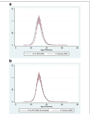
13Using the average age difference between fathers and sons from the national census,
the potential fathers’ age range in 1985 is set to 35–50 when the sons were 14, which covers around 95% of the father-son pairs. Appendix: Table 6 demonstrates age differ-ences between fathers and sons, and it is clear that statistics for KLIPS 2005 and National Census 2005 are closely similar; this can be verified easily in Appendix: Figure 1. This evi-dence justifies the use of KLIPS 2008 as a representative sample and restriction of samples based on the age information from KLIPS 2008.
14In fact, for sons 35–50 in 2008, their possible fathers were 34–68 in 1985; this covers
95% of fathers based on age difference information from census data in 2005. If I match the age range of 35–50 for fathers in 1985, I lose 20% of the sample; however, the estimates are similar. More information is provided in the next section.
15Between household head and non-head sons, differences exist in earnings and
endogenous selection. Moreover, there is no formal requirement to answer as a head but it is who represents the household. Thus, I included all male workers and presented the results for both samples. In addition, the national unemployment rate in Korea is around 5% in late 1980s and around 3.5% in 2000s, indicating that the excluded unemployed population is not troublesome.
16Note that estimates of age controls such as age and age squared of fathers are not
used to generate fathers’ missing earnings. This is because I am not predicting earnings at a particular age but am trying to predict fathers’ long-run earnings, which requires the standardization on ages.
17First, I draw a bootstrap sample of fathers from KLIPS 2003 and run equation (4) to
estimate parameters. Then I draw another bootstrap sample of sons from KLIPS 2006, from whose recollections data is used to generate fathers’ earnings. I estimateρ1in Eq. (5) and save estimates for 1000 replications. Murphy and Topel (1985) and Pagan (1984) showed that standard two-step procedures not accounting for generated regressor prob-lems underestimate standard errors of the consistent second-step estimators and that corrected standard errors are larger than their uncorrected counterparts. If a researcher ignores the fact that fathers’ earnings are generated and uses a bootstrap only in the sec-ond step, then standard errors are smaller than our approach, bootstrapping both steps, but still larger than those without bootstrapping in OLS.
18Key father’s earnings predictors are chosen to maximizeR2of the first-stage
regres-sion, and the results are summarized in Table 4. The adjustedR2in the first stage, 0.393, is relatively larger than the other studies in Table 5: Piraino (2007) with 0.322, Mocetti (2007) with 0.301, Nicoletti and Ermisch (2008) with 0.289, and Ueda (2013) with 0.23. Preferred first-step regression results are summarized in Appendix: Table 7 with an age range of 35–50 for both generations using all three earnings predictors.
19If I match the age range of 34–68 for potential fathers in 1985 covering 95% of the
father-son pairs, the estimate is 0.397, very similar to the estimate in the baseline model. Thus, hereafter, the age range of fathers in 1985 is fixed at 35–50 instead of 34–68. When self-employed sons are excluded, the sample size decreases to 502, and the esti-mate is 0.409 (0.064). Further analysis shows that the estiesti-mate is robust to the treatment on the self-employed workers. Results are available upon request. In addition, for house-hold heads, the sample size is 572 and ρˆ1 is 0.351 (0.062). Heads earn approximately 15 to 30% more than non-head members, and this might result in a relatively lower estimate.
20If I exclude the agriculture sector in industry and in occupation categories, which
mostly considers the sample residing in urban areas, the estimate is 0.337, the lowest among all models. It is reasonable to conjecture that the intergenerational mobil-ity is higher in urban areas than in rural areas, accounting for job opportunities in those areas.
21Key comparable countries in Table 5 have different age ranges for fathers and sons
22Hertz et al. (2008) documented the international comparison of educational
inheri-tance for sons 20–69. Some noticeable countries in Table 5 are Brazil (0.59), Chile (0.6), China (rural, 0.2), Italy (0.54), Sweden (0.4), UK (0.31), and USA (0.46).
23Real GDP per capita in Korea increased more than three times between 1985 and
2003, implying that the potential fathers’ cohort in 1985, which is more proximal to actual fathers, is different from the cohorts in 2003.
24(a)D
0 ≡ plimn→∞N−1Ni=1xˆ
ixˆi = E(xx), (b)f(·)is twice continuously
differen-tiable inθ for eachx1with the sample second moments of∂f/∂θ uniformly bounded in the sense of plimn→∞
N−1Ni=1xˆixˆi N−1Ni=1∇θf(x1,θ)ξi
=D1, where∇θf(x1,θ) is theK×QJacobian off(x1,θ), and (c)θˆis a consistent estimator ofθ.
25See chapters 6 and 12 in Wooldridge (2010) for details.
Appendix
I derive the consistency of OLS estimatorρ1in Eq. (7), where the dependent variable has a measurement error due to using the proxy and the independent variable is generated from an auxiliary regression.
yit=ρ1xˆi+ωit (7)
whereωitis equal toλti+νit+λtρ0+h(Ageit)+(λt−1)ρ1xˆi+λtρ1(xi− ˆxi).
Write Eq. (1) as
y=xρ+u (8)
where x = f(x1,θ), x1is a vector of variables from the first step that determines the unobservables,f(·), which is a 1×K vector of functions determined by the unknown vectorθ, which isQ×1. Assume thatE(u|x1) = 0 and errors are independent across observations. Further assume thatθˆis a√N-consistent estimator ofθ. Now letρˆbe the OLS estimator from the equation
yi= ˆxiρ+errori (9)
wherexˆi=f
x1i,θˆ
and errori=ui+
xi− ˆxi
ρ, the ordinary least squares estimator is
ˆ ρ=
N
i=1
ˆ xixˆi
−1 N
i=1
ˆ xiyi
(10)
Write yi = ˆxiρ +
xi− ˆxi
ρ +ui, where xi = f(x1i,θ), then plugging this in and
√
Nρˆ−λtρ
=
N−1 N
i=1
ˆ xixˆi
−1 N−1/2
N
i=1
ˆ
xixi− ˆxi
λtρ+ξi
(11)
whereξi=λti+νit+λtρ0+h(Ageit).
Under the regularity condition stated in theorem 1 in Murphy and Topel (1985) or theorem 12.3 in Wooldridge (2010),24a mean value expansion ofθˆgives
N−1/2 N
i=1
ˆ
xiξi=N−1/2 N
i=1 xiξi+
N−1 N
i=1
∇θf(x1,θ)ξi
√ N
ˆ
θ−θ+op(1) (12)
BecauseE
∇θf(x1,θ)ξi
= 0, it follows thatN−1Ni=1∇θf(x1,θ)ξi =op(1), and since √
N(θˆ−θ)=Op(1),
N−1/2 N
i=1
ˆ
xiξi=N−1/2 N
i=1
xiξi+op(1) (13)
Using similar reasoning, by mean value expansion
N−1/2 N
i=1
ˆ
xixi− ˆxi
λtρ= −
N−1 N
i=1 (ρ⊗xi)
∇θf(x1,θ)
√
N(θˆ−θ)+op(1) (14)
Now assume that
√
N(θˆ−θ)=N−1/2 N
i=1
ri(θ)+op(1) (15)
where I assumeE[ri(θ)]=0, which even holds for most estimators in nonlinear models.25
If I assume that Cov(xi,h(Ageit))=0, then
plimn→∞ρˆ= λtρVar(xi)+Cov(xi,νit) Var(xi)
(16)
which reduces toλtρif Cov(xi,νit) = 0. For consistency, replacingxiwithxˆiin an OLS
Table 6Father-son age difference
Census 2005 KLIPS 2005 KLIPS 2006 KLIPS 2008 Observation 139,832 2654 2655 2564 Average age difference 30.54 29.79 29.74 29.79 Standard deviation 4.25 4.25 4.22 4.21 Age range for 90% of observation 24–39 23–37 23–37 23–37 Age range for 95% of observation 22–41 22–39 22–39 22–39
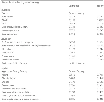
Table 7First-step regression
Dependent variable: log father’s earnings
Coefficient Std. err Education
None Omitted dummy
Elementary 0.2164 0.1032
Middle 0.3199 0.0999
High 0.4578 0.1006
Community college (2 years) 0.7388 0.1230 University (4 years) 0.7712 0.1043 Graduate school 0.7910 0.1313 Occupation
Professional, technical, managerial 0.0735 0.1301 Administrative and government officer, entrepreneur 0.0315 0.1923 Clerical worker 0.1172 0.1247 Sales worker 0.3916 0.1272 Service worker 0.3992 0.1415 Production worker 0.3119 0.1243 Agriculture, fishing, forestry Omitted dummy
Industry
Agriculture, fishing, forestry Omitted Dummy
Mining 0.2536 0.1711
Manufacturing 0.4053 0.1452 Utilities 0.4392 0.1933 Construction 0.1701 0.1486 Wholesale and retail trade 0.3348 0.1503 Communication, transportation 0.3703 0.1478 Banking, insurance, business service 0.3956 0.1547 Community, social, and personal services 0.3885 0.1445
Note: Age of the father-son sample is restricted to 35–50
Acknowledgements
I would like to thank Gary Solon, Steven Haider, and Chris Ahlin for helpful comments and sharing their insights. I am also grateful for comments and suggestions from seminar participants at the Canadian Economics Association, Midwest Economics Association, and Michigan State University.
I would also like to thank the anonymous referee and the editor for the useful remarks. Responsible editor: David Lam
Competing interests
The IZA Journal of Development and Migration is committed to the IZA Guiding Principles of Research Integrity. The author declares that he has observed these principles.
Publisher’s Note
Springer Nature remains neutral with regard to jurisdictional claims in published maps and institutional affiliations.
Received: 11 May 2017 Accepted: 23 May 2017
References
Björklund A, Jäntti M. Intergenerational income mobility and the role of family background. In: Oxford Handbook of Economic Inequality. Oxford: Oxford University Press. 2009. p. 491–521.
Björklund A, Jäntti M. Intergenerational income mobility in Sweden compared to the United States. Am Econ Rev. 1997;87(5):1009–18.
Black SE, Devereux P. Recent developments in intergenerational mobility. Handb Labor Econ. 2010.
Blanden J, Haveman R, Smeeding T, Wilson K. Intergenerational mobility in the United States and Great Britain: A comparative study of parent-child pathways. Rev Income Wealth. 2014;60(3):425–49.
Bowles S, Gintis H. The inheritance of inequality. J Econ Perspect. 2002;16(3):3–30.
Brenner J. Life-cycle variations in the association between current and lifetime earnings: evidence for German natives and guest workers. Labour Econ. 2010;17(2):392–406.
Cervini-Plá M. Exploring the sources of earnings transmission in Spain. Hacienda pública española. 2013:45–66. Choi J, Hong GS. An analysis of intergenerational earnings mobility in Korea: father-son correlation in labor earnings.
Korean Soc Secur Stud. 2011;27(3):143–63.
Dunn CE. The intergenerational transmission of lifetime earnings: evidence from Brazil. BE J Econ Anal Policy. 2007.;7(2). Fortin NM, Lefebvre S. Intergenerational income mobility in Canada. In: Labour Markets, Social Institutions, and the
Future of Canada’s Children. 1998. p. 89–553.
Francesconi M, Nicoletti C. Intergenerational mobility and sample selection in short panels. J Appl Econ. 2006;21(8): 1265–93.
Gong H, Leigh A, Meng X. Intergenerational income mobility in urban China. Rev Income Wealth. 2012;58(3):481–503. Grawe ND. Lifecycle bias in estimates of intergenerational earnings persistence. Labour Econ. 2006;13(5):551–70. Haider S, Solon G. Life-cycle variation in the association between current and lifetime earnings. Am Econ Rev. 2006;96:
1308–20.
Hertz T, Jayasundera T, Piraino P, Selcuk S, Smith N, Verashchagina A. The inheritance of educational inequality: international comparisons and fifty-year trends. BE J Econ Anal Policy. 2008.;7(2).
Kim H. An Analysis of intergenerational economic mobility in Korea. Korea Development Institute. 2009. R of Korea. Ministry of Education: Educational development in Korea 1988–1990; 1991. Report for the International
Bureau of Education, Geneva. Seoul: Korean National Commission for UNESCO.
Lefranc A. Educational expansion, earnings compression and changes in intergenerational economic mobility: Evidence from French cohorts. 20111931–1976. Unpublished manuscript, University of Cergy.
Lefranc A, Ojima F, Yoshida T. Intergenerational earnings mobility in Japan among sons and daughters: levels and trends. J Popul Econ. 2014;27(1):91–134.
Leigh A. Intergenerational mobility in Australia. BE J Econ Anal Policy. 2007.;7(2). Mocetti S. Intergenerational earnings mobility in Italy. BE J Econ Anal Policy. 2007.;7(2).
Murphy KM, Topel RH. Estimation and inference in two-step econometric models. J Bus Econ Stat. 1985;3:370–9. Nicoletti C, Ermisch J. Intergenerational earnings mobility: changes across cohorts in Britain. BE J Econ Anal Policy.
2008.;7(2).
Núñez J, Miranda L. Intergenerational income and educational mobility in urban Chile. Estud Econ. 2011;38(1):196–221. Nybom M, Stuhler J. Heterogeneous income profiles and lifecycle bias in intergenerational mobility estimation. J Hum
Resour. 2016;51(1):239.
Pagan A. Econometric issues in the analysis of regressions with generated regressors. Int Econ Rev. 1984;25:221–47. Piraino P. Comparable estimates of intergenerational income mobility in Italy. BE J Econ Anal Policy. 2007.;7(2). Solon G. Cross-country differences in intergenerational earnings mobility. J Econ Perspect. 2002;16:59–66. Solon G. Intergenerational mobility in the labor market. Handb Labor Econ. 1999.
Solon G. Intergenerational income mobility in the United States. Am Econ Rev. 1992;82:393–408. Ueda A. Intergenerational mobility of earnings in South Korea. J Asian Econ. 2013:1–22.