R E S E A R C H
Open Access
Agricultural contracts, adverse selection,
and multiple inputs
Rachael Goodhue
1*and Leo Simon
2,3*Correspondence:
[email protected] 1Department of Agricultural and Resource Economics, University of California, Davis, One Shields Avenue, Davis, CA 95616, USA Full list of author information is available at the end of the article
Abstract
A significant and growing share of US agricultural output is produced under a production or marketing contract. An important controversy regarding agricultural production contracts is the control of non-labor inputs. Over time, contracts have tended to place more inputs under the buyer’s control and fewer under the farmer’s. This analysis examines the welfare effects of this trend. In the framework considered here, returns are reduced for some farmers and left unaffected for others. Returns to the buyer increase. The net effect on total surplus has two components. Output is higher when the buyer controls the input, due to lower information rents accruing to more productive farmers. However, this reduction distorts input use away from the production cost-minimizing level, which is costly. The net effect on total surplus depends primarily on the elasticity of substitution between inputs. Given the limited substitutability between labor and non-labor inputs in many agricultural activities, the analysis suggests that greater control of non-labor inputs by the buyer increases total surplus. The increase in returns to the buyer is consistent with the growing share of output produced under vertical coordination and the tendency to specify a greater number of production activities rather than allowing farmers to make their own decisions. The reduction in the returns obtained by some farmers is consistent with farmers’ opposition to such requirements.
Keywords: Adverse selection, Agricultural contracts, Asymmetric information, Principal-agent theory, Production contracts, Vertical coordination
Background
Worldwide, many agricultural markets cannot be characterized as spot markets. A tremendous variety of forms of vertical coordination govern relationships between farm-ers and their buyfarm-ers. One type of coordination is a production contract. Production contracts between farmers and buyers specify allowable fertilizers, seedstock, produc-tion practices, and other inputs. Under some contracts the buyer may retain ownership of a key input, such as chickens in broiler chicken contracts and the seed and output in crop contracts. In others, such as processing tomato contracts, the buyer may restrict the set of permissible pesticides. Our analysis focuses on US production contracts as defined by the National Agricultural Statistics Service (2014) for the Census of Agriculture: ones which set “terms, conditions, and fees to be paid by the contractor to the operation for the production of crops, livestock, or poultry.” Production contracts account for a significant share of the value of agricultural output in the USA (16.8 % in 2008). Farmers may choose
to enter a production contract for a variety of reasons, such as a lower need for operating capital because the buyer provides some inputs, access to technical assistance provided by the buyer, or risk management. Often, the farmer’s contracting decision may have more than one reason. We examine one motivation for buyers, such as meatpackers, seed com-panies, and processors, to use production contracts when coordinating production with farmers.
While there are a number of reasons why a buyer may choose to control inputs that could just as easily be chosen by the farmer, this paper focuses on an information-driven motivation: the reduction of information rents arising from adverse selection and the resulting increase in profits. Information rents are the rents which are captured by a high ability farmer because his ability (type) is his private information. We examine the effects of who controls inputs in a framework in which output is a function of the farmer’s type and the levels of inputs he uses. The farmer’s type, his private information, affects the productivity of his effort, which is not observable, and of a non-labor input which the buyer observes only if she provides or specifies it as part of a production contract. We compare output and input levels, farmer compensation, buyer profits and total surplus under a contract which specifies that the buyer controls the input (“restrictive contract") with one in which the farmer controls it (“basic contract”). We then identify how the effects depend on the nature of the production process as characterized by the elasticity of substitution between non-labor inputs and the farmer’s effort.
The use of contracts differs across commodities. Some commodities use primarily pro-duction contracts, some use marketing contracts and others have little use of contracts of any type.1With the exception of dairy production, for which contracts are mostly market-ing contracts, the majority of contracts in livestock production are production contracts. A smaller share of crops are under contract, and most contracts are marketing contracts (O’Donoghue et al. 2011). The use of contracts also varies by farm size; large commercial farms are more likely to use production and/or marketing contracts and to use contracts for a larger share of their production (MacDonald and Korb 2011; MacDonald et al. 2004). Within livestock production, the use of production contracts varies. The two sec-tors with the most intensive use of contracts are broiler chickens and hogs. In 2011, 97 % of broilers were produced under contract, and 94 % of these contracts used con-tained provisions linking compensation to grower performance (MacDonald 2014).2 Generally, buyers, known as integrators, provide chicks, feed, veterinary services, trans-portation services, and technical advice to growers. Additionally, they include specific requirements regarding housing in the contracts. Requirements are not limited to initial construction; 29 % of respondents to the 2011 USDA Agricultural Resources Manage-ment Survey reported incurring capital expenditures required by their integrators in 2009–2011 (MacDonald 2014).
The farmer receives a fee and the contractor receives the residual returns. The farmer’s return includes a payment based on the number of hogs or capacity. It may include incen-tive clauses regarding feed efficiency (MacDonald and McBride 2009). Key and McBride (2003) find that production contracts notably increase the productivity of US feeder-pig-to-finish hog operations. Key and McBride (2008) find that there was a substantial increase in total factor productivity in the U.S. hog industry between 1992 and 2004, due mostly to technical progress and increased scale efficiencies. This finding is consistent with contract use and contract provisions influencing productivity due to which farmers contract and the design of these contracts.
Variations in the use of contracts across commodities and regions suggest that there are many factors which influence contract choice. Here, we provide a few examples. Con-sider the case of a supermarket chain entering a developing country and deciding how to procure fresh produce. It may elect to use a production contract with local farmers or farmers’ organizations in order to provide seed, fertilizer, and technical education because local producers cannot deliver produce of the chain’s desired quality with local inputs or, perhaps due to credit constraints, cannot purchase sufficient inputs. On the other hand, a supermarket chain in a developed country may elect to use a marketing contract because its domestic producers can deliver produce of the requisite quality. Although the contract-ing parties and the output are the same in these cases, in one case a farmer cannot produce that output without input provision by the buyer. In this example, an off-setting consid-eration might be differences in contract enforcement due to differences in the strength of the legal system.
Alternative means of providing information may reduce the need for contracts. For example, public or third-party grading standards that evaluate all verifiable product char-acteristics of value to buyers at the time of delivery can substitute for a marketing contract that specifies these same requirements. In instances in which grading standards address all relevant characteristics, there is less of an incentive to use marketing contracts rather than the spot market.
Product perishability is another consideration. When a product is highly perishable, then a contract with a buyer ensures the farmer that he can place his output while it still has market value. Subject to the vagaries of weather, contracting also ensures the buyer that she will have a consistent stream of deliveries. This is an important consider-ation for retailers and for processors. Whether or not these considerconsider-ations indicate that a production contract should be selected rather than a marketing contract will in turn be influenced by other factors, such as those discussed above. When a product is storable, timing and consistent deliveries are less important factors.
Clearly, no single factor motivates all contract choices. This analysis focuses on one motivation for using production contracts: the buyer can reduce the information rents obtained by high ability farmers by designing a production contract menu for farmers of different abilities that specifies or provides non-labor inputs, as well as output, for farmers of each type.
presented here. Goodhue (2000) demonstrates that when there is an adverse selection problem, the buyer can reduce information rents by controlling non-labor inputs used in the restrictive case of a Cobb-Douglas production function. Unlike the analysis here, she compares the two conventional cases of complete information and “pure” asym-metric information where the buyer has zero information regarding the farmer’s use of the non-labor input unless the buyer controls the input. In contrast, by introduc-ing a continuous degree of asymmetric information we can use comparative statics to examine the properties of the buyer’s profit-maximizing solution. Just et al. (2005) focus on the effect of sharing technologies when firms may choose to integrate horizontally. Unlike the non-cooperative solution concept considered here, they consider a coopera-tive solution. Using the Nash bargaining solution, they find that the gains from horizontal integration increase with the degree of differences in firms’ production technologies and endowments.
There is a fairly small empirical literature regarding the use of input control by the buyer in agricultural contracts. Within this literature, the four articles which address questions most closely related to our analysis are Knoeber and Thurman (1995), Martin (1997), Thomsen et al. (2004), and Goodhue et al. (2003). Knoeber and Thurman (1995) examine how provisions in broiler contracts alter the per-flock risks borne by farmers and by pro-cessors (commonly known as integrators in this industry) compared to the spot market, using spot market prices and a dataset on broiler contract outcomes. They find that the majority of risk is transferred from farmers to integrators, including price risk and rela-tive production risk. Price risk accounts for the majority of risk transferred. Martin (1997) performs a similar analysis of hog contracts. Thomsen et al. (2004) consider the effect of placement risk, defined as how often flocks are placed with growers, on grower returns. Goodhue et al. (2003) examine the determinants of the use of input control provisions in California winegrape contracts and find that these provisions are more commonly used in regions which produce higher quality winegrapes. Fraser (2005) finds similar results for contracts in the Australian wine industry.
non-labor input. The difference is due to two assumptions that differ from ours: (a) the principal always has the possibility to choose to observe inputs purchased by the agent; and (b) the timing of their model, especially the possibility of renegotiation after the agent chooses capital but before production occurs. We assume that capital and effort are chosen simultaneously, and that production is realized without an opportunity for renegotiation.
Of course, the model developed here is only one possible explanation for buyers’ adop-tion of input control provisions. There are many other reasons why buyers may choose to adopt input control provisions in agricultural contracts (Goodhue 1999; Hueth et al. 1999). Some, but not all, involve asymmetric information. Some instances of asymmetric information may arise in a buyer-farmer relationship involving multiple inputs. For exam-ple, the buyer may be less informed than the farmer regarding the precise nature of the production function. When information is asymmetric in this sense, it may be costly for the buyer to determine the input mix: she may select a combination that the farmer could improve upon. There may be a moral hazard problem if the farmer’s effort is unobserv-able in terms of its effects on quantity or product quality and the effect is dependent on the use of other inputs (Sexton 2013). Other motivations for input provision based on the farmer’s characteristics include relaxing a liquidity constraint if he is credit constrained or redistributing risk if he is risk averse. Quality considerations, including but not limited to ones involving asymmetric information, are also important. Contracts, including ones with input control provisions, can aid planning of the production process for the buyer in terms of obtaining sufficient product with the desired quality attributes to ensure consis-tency, as well as simply in terms of timing deliveries to manage throughput, even in the absence of asymmetric information (Jang and Olson 2010; Wilson and Dahl 1999; Worley and McCluskey 2000).
Under an agricultural contract, the change in which party controls key inputs and/or other production decisions alters the distribution of risks and returns to the farmer and buyer relative to those associated with the spot market. We focus on the change in the distribution of returns and total surplus due to differences in who controls non-labor inputs. In order to do so, we introduce a theoretical construction which continuously varies the degree of asymmetric information in the buyer’s maximization problem.
Our approach is similar in some technical respects to the use of marginal analysis of the share of informed farmers as a measure of the asymmetric information facing market makers in the market microstructure literature examining bid-ask spreads, e.g. Copeland and Galai (1983), Glosten and Milgrom (1985), and Kyle (1985). However, our approach differs from Khalil and Lawarree (2001) and these studies conceptually due to our differ-ent context and research question; because we are interested in the total cost of a specific degree of asymmetric information, not just its marginal cost, we integrate the results of our marginal analysis over specified intervals in order to analyze the total impacts of a given degree of asymmetric information.
The net effect of these differences between the contract types for society as a whole is less clear. We establish that if the elasticity of substitution between effort and the other input is sufficiently small, the restrictive contract will result in higher total surplus than the basic contract. If the elasticity of substitution is large, the welfare comparison depends on the relative importance of the output and the input mix distortions. These findings contribute to the property rights literature regarding how the boundaries and the allo-cation of decision rights affect the ex post-efficiency of production (Coase 1937; Tirole 1999; Williamson 1985). The analysis has a specific implication in our context; because there is limited substitutability between labor and inputs such as seed animals, or facili-ties in agricultural production, it is most likely the case that higher total surplus results when buyers, rather than farmers, control non-labor inputs in agricultural contracts.
These findings provide a strong motivation for the buyer to increase the degree of integration; that is, one must look outside our framework to justify a decision by the buyer to allow the farmer to make input allocation decisions rather than controlling them herself. Moreover, the model provides one explanation of why buyers are choosing to source an increasing share of their purchases through integrated production and con-tracts specifying non-labor inputs: by doing so, buyers can reduce the information rents that they need to pay. Conversely, it suggests a reason for the widespread opposition by farmers to increased coordination (Vavra 2009): highly productive farmers do not want the information rents they can command to be reduced by greater buyer control over production.
Methods
We begin with a standard principal-agent model. The farmer, who is the agent, may be one of two types; each type has access to a distinct production function, and one type’s function is more productive than the other. Both the buyer (principal) and farmer are perfectly informed about the specification of these functions and the probability distri-bution over types. The farmer’s realized type, however, is unknown to the buyer. The buyer’s goal is to maximize her profits from production, which depend on the farmer’s production possibilities. To induce the farmer to reveal his true type, she must offer him a menu of two contracts, one designed for each type, that provides him with adequate incentives to do so. We assume that the buyer cannot observe the level of effort supplied by the farmer. We compare two cases: one in which capital is observable and non-verifiable and one in which it is observable and non-verifiable. For expository convenience, we refer to non-observable capital as capital supplied by the farmer and observable capital as capital supplied by the buyer. We assume that capital is homogeneous, so that only the level of capital and the production set available to the farmer who uses it are relevant to production.
The production function: Production depends on capital (k), effort (e), and the farmer’s type (θ). There are two types, “low” and “high,” denoted byandh. The farmer’s true type isθ ∈ {θ,θh}. Let= θ
θh <1, reflecting the fact thatis less efficient thanh. For i=,h, letφidenote the probability that a farmer’s type isi. (Obviously,φ+φh=1).
We impose the following additional assumptions on the production function,f(e,k;θ).
A1: There exists a twice continuously differentiable function,g:R2→R, such that for
A2: The functiongis homogeneous of degreeα <1ineandk;
A3: The marginal products of effort and capital,geandgk, are positive, andgis strictly
concave in(e,k), (i.e.,gee,gkk <0andgee,gkk > (gek)2).
For i = {,h}, we shall usually write fi rather than f(·,·,θi). For convenience, we will normalize by setting θ = 1, so that f ≡ g. Assumption A1 implies that θ is “technologically neutral,” in the sense that for eacheandk, fe(e,k)
fk(e,k) =
fh e(e,k)
fkh(e,k).
4
Farmer’s decision: The farmer receives a lump-sum transfer payment from the buyer and in return delivers a specified level of output, contributing effort and, in one of our two cases, capital. The farmer’s outside alternative is to provide his effort at the given wage ratew > 0 per unit effort supplied. The wage rate exactly compensates for the farmer’s constant marginal disutility of effort, so that his reservation utility when he does not supply effort is zero. The price of capital is constant atr > 0 per unit. In order to induce the farmer to supply effort leveleand capital levelk, the buyer’s transfer payment must at least cover the farmer’s cost,we+rk.
Input levels: If a farmer of type θ chooses input levels to produce a givenq—i.e., if the buyer cannot observe and verify capital levels—he will solve the (neo-classical) cost minimization problem min
e,k we+rk s.t.f(e,k,θ) = q. Let
˜
e(q,θ),k˜(q,θ)
denote the
solution to this problem.
We will refer to this input vector as theneoclassical input mix for q. The solution to the farmer’s problem exhibits the following, well-known properties:
Remark 1The neoclassical input mix is uniquely defined by the first-order condition:
0 = wfk
˜
e(q,θ),k˜(q,θ),θ
− rfe
˜
e(q,θ),k˜(q,θ),θ
. (1)
Moreover, there exists a constantβ˜ such that for all q, k˜˜e((··,,θθ)) = ˜β. Finally, for all q,
˜
e(q,θ),k˜(q,θ)=1/αe˜(q,θh),k˜(q,θh).
Uniqueness follows from the strict concavity ofg(A3). Linearity of farmer’s expan-sion path follows from homogeneity (A2) and the fact thatrandware constants. The proportionality relationship between different types’ input vectors follows from A1 and A2.
LetC˜P(q,θ)denote typeθ’sproduction costof delivering outputqwith the neoclassical input mix:
˜
CP(q,θ) = w˜e(q,θ) + rk˜(q,θ). (2)
An immediate consequence of Remark 1 is that when the farmer chooses inputs, there is an equivalent,single-inputcharacterization of technology,f¨(e,¨ θ)= ¨eαf(1,β˜,θ), and of production costs,C¨P(q,θ) = ¨ve¨(q,θ), where each unit of thecompositeinpute¨is
com-posed of one unit ofeandβ˜units ofk, and¨v=(v+ ˜βr)denotes the unit cost of¨e. Provided that the input mix is always neo-classical, this alternative characterization is equivalent to the original one in the following sense:
Remark 2For each q and θ,¨f(e¨(q,θ),θ) = f
˜
e(q,θ),k˜(q,θ),θ
and ¨
The significance of Remark 2 is that when the farmer chooses inputs, the buyer’s prob-lem in our two-input model is formally equivalent to the corresponding, and routine, textbook problem, in which technology is given by the single-input production function ¨
f with constant unit cost¨v.
Now assume instead that the buyer chooses the level of capital, lete¯denote the level of effort required to produceqgivenkandθ, and letC¯P(q,k,θ)denoteθ’s production cost
of deliveringqusingk:
¯
CP(q,k,θ) = we¯(q,k,θ) + rk. (3)
The cost to farmer-typeof producing any level of output is strictly larger than the cost to typeh.
Contracts: Abasic contractis one in which the farmer chooses both inputs. A menu of basic contracts assigns to each announced typeθi,i∈ {,h}, an output level and transfer,
˜
q(θi),˜t(θi). We will sometimes write the contract menuq˜(θi),˜t(θi)i=,has(q˜,˜t) =
(q˜,˜t),(q˜h,˜th)
. Arestrictive contractis one in which the buyer specifies capital and the farmer chooses labor. A menu of restrictive contracts assigns to eachθian output level,
capital level, and transfer. We will similarly sometimes write
¯
q(θi),k¯(θi),¯t(θi)
i=,has
(q¯,k¯,t¯)=
(q¯,k¯,¯t),(q¯h,k¯h,¯th). Invoking the revelation principle (Myerson 1979), we
restrict our analysis to truth-telling contracts in which each farmer chooses to announce his true type by selecting the contract for his type from the menu of two contracts offered by the buyer.
Timing and information: Regardless of contract type, the timing of the game is as fol-lows: The buyer offers a contract menu to the farmer on a take-it-or-leave-it basis. At the time the contract menu is offered, the farmer’s type is his private information. The probability of each type occurring is common knowledge. We assume that if the farmer is indifferent between accepting and not accepting a contract then he will accept the con-tract. Similarly, we assume if he is indifferent between the two contracts, he will choose the contract intended for his true type. Production and transfers are then implemented according to contract specifications. The buyer then sells her output on a competitive market.
Symmetric information benchmark: We assume throughout that output is sold on a perfectly competitive market at a price ofp. Forθ ∈ {θ,θh}, letq(θ)denote the level
of output satisfying dC˜P(qdq(θ),θ) = p. Also, let(e(θ),k(θ)) = (e˜(q(θ),θ),k˜(q(θ),θ)) denote the neoclassical input mix forq(θ). If the buyerwereable to observe the farmer’s type, the solution to the buyer’s profit maximization problem would be to specify the out-put pairq(·), whether or not she chose capital levels. Regardless of who chose the level of capital, the farmer of typeθ would then produceq(θ)with inputs(e(θ),k(θ)). We shall refer to(q,e,k)as thesymmetric information benchmark solution. Assumptions A1–A3 ensure that in the benchmark solution both types produce a positive quantity.
Results and discussion
driving differences in outcomes under the two contracts, we conduct a marginal anal-ysis by continuously varying the degree of asymmetric information between symmetric information and the standard model. The marginal analysis identifies the factors which influence profits and total surplus as the degree of information asymmetry increases. In the context of production contracts, it identifies the value to the buyer of reducing asymmetric information by imposing additional constraints on production decisions.
Buyer’s profit-maximizing basic and restrictive contracts
This subsection develops the buyer’s profit-maximizing basic and restrictive contracts and then compares output, information rents, production costs, and profits under the two contracts.
Buyer’s profit-maximizing basic contract
Given a menu of basic contracts(q˜,˜t), the buyer’s profit when the farmer declares a type of θˆ ispq˜(θ)ˆ − ˜t(θ)ˆ . Thus, the buyer’s problem is to choose the contract menu (q˜,˜t)
that maximizesi∈{,h}φipq˜(θi)− ˜t(θi) subject to incentive and participation con-straints. Because the principal’s problem when there is a basic contract is the same as one with a single composite input, we can characterize the optimal basic contract menu by drawing on standard results from the mechanism design literature in which produc-tion is a funcproduc-tion of the farmer’s effort: the constraints that are binding on the buyer are typeh’s incentive compatibility constraint and type’s individual rationality constraint. Consequently,hand produce, respectively, at and below the symmetric information benchmark solution levels for their types. Moreover, the difference between the trans-fer oftrans-fered toand’s production cost of delivering the designated output level will just equal’s reservation utility, which in our model is zero. On the other hand, the transfer offered tohincludes a premium, referred to as hisinformation rent, which in the optimal contract will just offset the increment in utility thathwould derive by adopting’s con-tract rather than the one intended for him. Remark 3 summarizes the textbook treatment of this class of contract (see, e.g., Varian 1992, pp. 457–463).
Remark 3The optimal basic contract menu has the following properties:
1. farmerproduces less than he does in the symmetric information benchmark, ˜
q<q(θ), and receives a transfer equal to his production costs:
˜
t = C˜P(q˜). (4a)
2. farmerhproduces the same quantity as in the symmetric information benchmark, ˜
qh=q(θh), and receives a transfer greater than his production costs:
˜
th = C˜Ph(q˜h) +
˜
CP(q˜) − C˜hP(q˜)
. (4b)
h’s transfer compensates him for his own production costs (the first term) plus pays him the difference between the transfer he would obtain for producingq˜and his cost of producing it (the difference between the second and third terms).
ensure truthful revelation by the buyer.6The terms “marginal production” and “marginal information” costs will then have the obvious interpretation.
Profit-maximizing restrictive contract
Given a restrictive contract menu(q¯,k¯,t¯), the buyer’s profit from a farmer declaring a type ofθˆispq¯(θ)ˆ −¯t(θ)ˆ . Thus, her problem is to choose the contract menu(q¯,k¯,¯t)that maximizesi∈{,h}φipq¯(θi)−¯t(θi)subject to incentive and participation constraints. Under a restrictive contract, the input mix is no longer exogenous to the buyer’s deci-sion. Consequently, the textbook single-input model can no longer be used to characterize the optimal restrictive contract menu. Instead, Lemma 1 below establishes that the prin-cipal’s constrained profit maximization problem is equivalent to an unconstrained profit maximization problem which substitutes into the principal’s expression for profits the two binding contraints: the low ability farmer’s reservation utility constraint and the high ability farmer’s incentive compatibility constraint.
Lemma 1The problem of choosing the optimal restrictive contract menu is equivalent to the following problem:
max (q¯,k¯)
i∈{,h}
φipq¯(θi)− ¯t(θi) (5)
where ¯th = C¯hP(q¯h,k¯h) + C¯P(q¯,k¯) − C¯hP(q¯,k¯)
¯
t = C¯P(q¯,k¯).
That is, any solution to(5)is a solution to the buyer’s restrictive problem and vice versa.
The proofs, and all subsequent ones, are deferred until the “Appendix”. Equipped with Lemma 1, we establish that the restrictive contract problem shares many of the properties of the single-input problem. Formally,
Proposition 1The optimal restrictive contract menu has the following properties:
1. farmerproduces less than he does in the symmetric information benchmark, ¯
q<q(θ), with capital levelk¯and receives a transfer equal to his production costs:
¯
t = C¯Pq¯,k¯.‘ (6a)
2. farmerhproduces the same quantity as in the symmetric information benchmark, ¯
qh=q(θh), using the neo-classical input vectore(θh),k(θh), and receives a transfer greater than his production costs:
¯
th = C¯hP
¯ qh
+ C¯P
¯ q,k¯
− C¯Ph
¯ q,k¯
. (6b)
h’s transfer compensates him for his own production costs (the first term) plus pays him the difference between the transfer he would obtain for producingq¯and his cost of producing it (the difference between the second and third terms). 3. farmer’s capital-effort ratio exceeds the neo-classical ratioβ˜.
that the task of choosing the optimal restrictive contract menu can be reformulated as the following (unconstrained) maximization problem:
max (q¯,k¯)
i∈{,h}
φipq¯(θi)− ¯CP(q¯(θi),k¯(θi),θi) + φhC¯I(q¯(θ),k¯(θ)). (7a)
Similarly, from Proposition 3, the task of choosing the optimal basic contract can be reformulated as
max ˜
q
i∈{,h}
φipq˜θi− ˜CPq˜θi,θi + φhC˜Iq˜θ (7b)
whereC˜I(q)= ˜CP
(q)− ˜ChP(q)denotes the information cost of contracting with typeto
producequnder a basic contract.
Because information costs are independent of typeh’s contractual variables, the pres-ence of information asymmetry has no impact onh’s choice of inputs or output, and hence cost of production, under either type of contract. Hence, all these values coincide with their symmetric information benchmark values. For this reason, we shall ignore this aspect of the buyer’s problem for the remainder of the paper and focus our attention on the contract targeted for type. Because information costs depend on the difference in productivity between the two types,hwill continue to be in the discussion.
To streamline notation,7we divide byφand writeφh/φas .
Basic: max ˜
q
pq˜− ˜CP
˜ q,θ
− C˜I(q˜). (7c)
Restrictive: max (q¯,k¯)
pq¯− ¯CPq,¯ k,¯ θ − C¯I(q¯). (7d)
Givenq, letC˜I(q) = ˜CP
(q)− ˜ChP(q)denote the information cost of havingqproduced
under a basic contract, when both types use the neo-classical input mix. For givenk, let ¯
CI(q,k) = ¯CP(q,k)− ¯ChP(q,k)denote the information cost of havingqproduced under a restrictive contract requiring the use of the capital levelk. The results which follow are consequences of the following inequality:8
for all positiveq, and allk≥ ˜kq,θ, C˜I(q) >C¯I(q,k). (8)
That is, the information cost associated with the profit-maximizing basic contract is always greater than the information cost associated with the profit-maximizing restrictive contract (which requires typeto utilize a super-optimal level of capital).
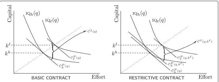
Figure 1 illustrates (8) by comparing a basic contract in which the farmer is required to produce an arbitrary output levelqagainst a restrictive contract in which the farmer is required to producequsing the neo-classical input mix for his type. The purpose of the figure is to show that the latter contract will be more profitable than the former. It is not, however, themostprofitable way for the buyer to obtainq: from part 3 of Proposition 1, the buyer can do even better than the illustrated restrictive contract if she requiresto choose a super-optimal capital-labor mix.
Fig. 1Information cost of producingqunder a basic contract vs. a restrictive contract
producesqusing the neo-classical input mix for his type (includingki). The brace in the right panel indicates the reduced cost differential when the contract designed for type specifically requires thatqmust be produced using the capital levelkthat is optimal for type; because of this restriction, if typehchose the contract for type, he would be obliged to use an excessive amount of capital. (A sufficient condition for the cost differen-tial to be smaller in the right panel than the left is that effort and capital are not perfectly substitutable.) The braces in the two panel also represent the respective information rents that the buyer must pay farmerhto produceq, under either a basic and restrictive con-tract: the input-mix penalty built into the restrictive contract lowers the incentive forh to “cheat” and pretend to beand hence also the incentive payment required to induce truthful revelation.
Figure 1 also demonstrates how the buyer can construct a restrictive contract which exactly mimics any basic contract, except for the added restriction on the input mix thath must use if she deviates from truthful behavior. The buyer’s revenues are the same under both contracts because outputs are the same. Production costs are also the same because, provided the farmer of typeichooses the contract designed for typei, the input mix he selects will be identical under the two contracts. But information rents are lower under the restrictive contract, and so profits associated withqare higher. Sinceqandkwere cho-sen arbitrarily, this argument applies in particular toq˜(θ), the output assigned toin the optimal basic contract. It follows that profits under this contract must be strictly less than profits he obtains by “mimicking”and choosing’s restrictive contract described above, and hence lower by an even greater margin than profits under theoptimal restrictive contract. The preceding remarks are summarized in Proposition 2.
Proposition 2The buyer’s profits under the optimal restrictive contract strictly exceed her profits under the optimal basic contract.
Marginal analysis of the basic and restrictive contracts
is replaced withγ. Whenγ = 0, the asymmetric information component of the buyer’s problem is eliminated, since the farmer is known to be of type. Now, we can use calcu-lus techniques to examine the impact of a small “increase in buyer uncertainty,”dγ. For each agent type, the symmetric information benchmark solution (p. 8) is independent of the type-probability ratioγ; consequently, the rates at which,conditional on each type, output, the buyer’s profits, etc. decline asγ increases are pure measures of themarginal impacts of buyer uncertainty. We then integrate these marginal impacts over the interval [ 0, ] to recover and compare thetotalimpacts of buyer uncertainty on the solutions to the buyer’s original problems (7c) and (7d).
Marginal analysis of the restrictive contract
We begin by determining the minimum cost to the buyer of having typeproduce at leastqunder a restrictive contract for a givenγ, while ensuring that typehdoes not have an incentive to pretend to be type. This cost minimization problem requires picking the nonnegative vector(e,k),e = e,eh, which minimizes theproduction cost(we+
rk)plus theexpected information costγwe−ehof producingqunder the restrictive
contract, subject to the constraints that (a) farmerproducesqusingk,eand (b) if farmerhselects the contract designed for, he producesqusingk,eh. Summarizing, the principal’s problem is
min (e,k)
w(1+γ )e−γeh+rk
Term A
s.t.f(e,k)=q,fh(eh,k)=qand(e,k)≥0. (9)
As a consequence of a restriction, we shall later impose (see (15) below), the solution values(e,k)for (9) are necessarily positive. Because of this, we will omit the nonnegativity constraints from our specification of the Lagrangian, which is
¯
L(e,k,λ;q,γ )=w
(1+γ )e−γeh
+rk+λ(q−f(e,k))+λh(fh(eh,k)−q)). (10)
where λ = (λ,λh) is the vector of multipliers for the restricted problem. Let
¯
e(q,γ ), ,kq,¯ γ ),λ¯q,γ )denote the solution to (9). Inserting these values into Term A of
(9), we obtain therestrictive cost function,C¯(q,γ )= ¯CP(q,γ )+ ¯Ci(q,γ ), whereC¯P(q,γ )=
(we¯(q,γ )+rk¯(q,γ ))is the production cost, andC¯i(q,γ )=γw(¯e(q,γ )− ¯eh(q,γ ))is the information cost of producingqunder the restrictive contract.
The first-order condition forL¯has five equations in five unknowns:
¯L = ⎡ ⎢ ⎢ ⎢ ⎢ ⎢ ⎢ ⎣ ¯ Le
¯ Leh
¯ Lk
¯ Lλ¯
¯ Lλ¯h
⎤ ⎥ ⎥ ⎥ ⎥ ⎥ ⎥ ⎦
= ⎡ ⎢ ⎢ ⎢ ⎢ ⎢ ⎢ ⎣
(1+γ )w− ¯λfe
−γw+ ¯λhfeh r− ¯λfk+ ¯λhfkh q−f(e,k) fh(eh,k)−q
⎤ ⎥ ⎥ ⎥ ⎥ ⎥ ⎥ ⎦
= 0. (11)
At the solution to (11),
¯
e(q,γ ),k¯(q,γ ),λ¯(q,γ )
, the constraints are identically zero
total cost under the restrictive contract for each(q,γ )pair—is identically equal to the minimized value ofL, henceforth denoted by¯ L¯(·;q,γ ).
Note that becauseL¯e,L¯eh, andL¯kare all zero, we have
¯
λ= (1+γ )w fe >λ¯
h= γw
fh e
. (12)
Substituting the expressions for theλ’s (Eq. (12)) into the expression forL¯k (eq. (11))
yields:
r w =
¯ fk ¯ fe +γ
¯ fk ¯ fe −
¯ fkh ¯ fh
e
. (13)
Becausehis more efficient thanand both use the same level of capital to produceq,h’s effort level under the restrictive contract must be less than’s. That is,e¯k¯ > e¯k¯h which in
turn impliesf¯k ¯
fe > ¯
fkh ¯
fh e
. Hence, the term in parentheses in (13) is positive, implyingf¯k ¯
fe <
r w.
Proposition 3 follows immediately.
Proposition 3In a restrictive contract for a given(q,γ ) 0, the prescribed capital-effort ratio for the low ability farmer is greater than the neoclassical ratioβ˜.
(For a vectorx∈Rn, we writex0 ifxi > 0, fori= 1, ...n). Note that Proposition 3
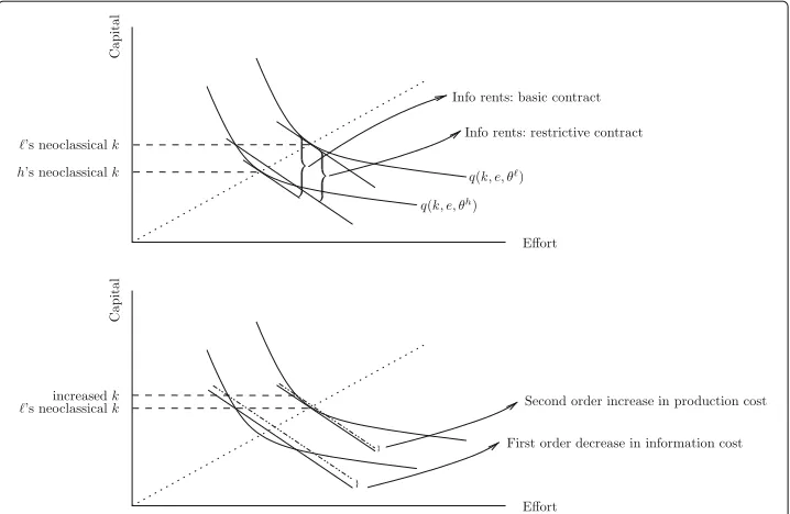
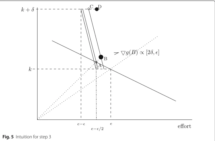
is more general than, and hence implies, property 3 of Proposition 1. Figure 2 provides intuition for Proposition 3. Its top panel reproduces Fig. 1 above. Consider the effect on the buyer’s problem of increasingγ from zero, for the moment holding the output level constant at an arbitrary output levelq. Whenγ =0, the typefarmer is required to use the neo-classical input mix. By the envelope theorem, a small increase in capital intensity above the neoclassical level has only a second-order impact on the production costs of farmer(see the bottom panel of Fig. 2). On the other hand, because the neo-classical klevel for farmeris super-optimal for farmerh, the given increase in capital intensity would result in afirst-order increase in farmerh’s production cost if he chose the contract designed for. Thus, a small increase in capital intensity beyond the neoclassical level forresults in a first-order reduction in information costs, and a second-order increase in production costs. It follows that wheneverγ > 0, the prescribed level of capital for farmerwill exceed the neoclassical level for her prescribed level of output.9
Therestrictive marginal cost function, denoted byMC, is identically equal to dL¯(·dq;q,γ ) which, by the envelope theorem, equals∂L¯(·∂;qq,γ ). This partial derivative in turn equals the difference between the two Lagrangians,λ¯andλ¯h, so thatMC(q,γ )= ¯λ(q,γ )−¯λh(q,γ ). Moreover, at the buyer’s optimum,MC(q¯(γ ),γ )=p, whereq¯(γ )is the profit maximizing level of output produced by the farmer of typeat pricepunder the restrictive contract.
Fig. 2Effects on production and information cost of increasing capital: basic vs. restrictive contract
Consider the case in which the production functiong is CES in addition to satisfying A1–A3. In this case, the expression for the determinant reduces to
HL(γ )= −τ ×
γ fh
e(eh,k)
efe(e,k) kfk(e,k) −
1+γ fe(e,k)
ehfeh(eh,k) kfkh(eh,k)
. (14)
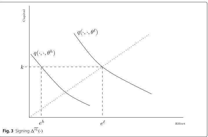
whereτ>0 depends only on parameters of the model. Clearly, expression (14) will be positive in a neighborhood ofγ=0. For largeγ, however, positivity is difficult to guarantee when inputs are close substitutes andhis much more efficient than. Figure 3 illustrates the problem. When isoquants have minimal curvature, the difference betweenfe(e,k) andfh
e(eh,k)depends on the efficiency gap, but only minimally on the input ratio, while
the ratiosefe(e,k)
kfk(e,k) and
ehfeh(eh,k)
kfh k(eh,k)
are very similar. Given all other parameters, therefore, we
can construct an example in whichehis arbitrarily close to zero (as in Fig. 3), ensuring that (14) will be positive except whenγ is very small. Lemma 2 establishes that this problem does not arise when the elasticity of substitution between effort and labor is bounded above by unity.10
Lemma 2If g is CES in effort and capital, with constant elasticity of substitution parameterσ¯ke≤1, thenHL(·)will be positive on[ 0, ].
Because the sufficient condition in Lemma 2 is far from necessary for the property we need, we will hold the condition in reserve for the moment and, in Propositions 4 and 6 below, simplyassumethatHL(·) >0. A convenient implication of this assumption— which we invoked when we specified the Lagragian (10)—is
For allγ >0, ifHL(γ )is positive then
Fig. 3SigningHL(·)
To see this, note that ifeh(q¯(γ ),γ )=0, the first term in (14) would be positive and the second term zero.
Proposition 4A sufficient condition for the restrictive marginal cost function MC(·,γ ) to be increasing in q, and forq¯(·)to be a continuously differentiable function ofγ, for all γ ∈[ 0, ], is that the determinant of the Hessian of the Lagrangian (10)is positive on [ 0, ]. Moreover,
¯
q(·)= w
¯ e− ¯eh
(α−1)(λ¯− ¯λh) <0. (16)
It is straightforward to verify, from (12) and (29), that if the ratio,γ, of high types to low types is sufficiently small, the determinant of the Hessian of the Lagrangian will indeed be positive.
Marginal analysis of the basic contract
In order to compare outcomes under the two contracts, we must obtain an expression fordq˜d(γ )γ . Remark 2, established that it is sufficient to analyze the equivalent single-input formulation of the buyer’s problem under the basic contract.
Letg¨denote the single-input production function corresponding tof. Let¨ei(q)denote the level of composite input required for typeito produceq.11From Remark 1,e¨h(·) =
1/α¨e(·)(recall from page 7 that = θ
θh), so that the information cost of producingq under a basic contract isC¨i(q)= ¨v1−1/αe¨(q). Thus, thebasic cost functionis
˜
C(q,γ ) = C¨P
q,θ
+ γC¨i(q) = v¨1+γ1−1/α¨e(q). (17)
Becausede¨dq(q) =g¨(¨e(q))−1, thebasic marginal cost functionis
MC(q,γ ) = v¨1+γ1−1/α g¨(e¨(q)) −1
The profit maximizing level of output,q˜(γ ), produced by the farmerat pricepunder the basic contract is defined by the conditionMC(q˜(γ ),γ ) = p. Applying the implicit function theorem,
dq˜(γ )
dγ = −
∂MC(q˜(γ ),γ ) ∂γ
∂MC(q˜(γ ),γ ) ∂q
= v¨1−1/α/g¨v¨
1+γ1−1/α
(g¨)2
¨ g
¨ g.
Euler’s theorem implies thatg¨=(α−1)g¨/e¨(q). becauseg¨is homogeneous of degree α−1. By profit maximization,1+γ1−1/α=pg¨/v. Using these two equalities,¨ the expression becomes
dq˜(γ )
dγ =
¨
v¨e(q)1−1/α
(α−1)p =
(we˜(q)+rk˜(q))1−1/α
(α−1)p < 0.
(19)
Comparing the marginal effects of the restrictive and basic contracts
This subsection establishes two factors that contribute to the dominance, from the buyer’s perspective, of the restrictive over the basic contract. Inequality (8) above established that information costs are lower under the the optimal restrictive contract than under the optimal basic contract; Proposition 3 established thatproductioncosts are higher. Proposition 5 demonstrates that the former inequality dominates.
Proposition 5For any given(q,γ ) 0, the buyer’s total cost of optimally obtaining q under a restrictive contract is less than the corresponding costs under a basic contract. That is,
for allqand allγ >0, C¯(q,γ ) < C˜(q,γ ). (20)
The proof of Proposition 5 is immediate: the neoclassical input mix is feasible under the restrictive contract, but, by Proposition 3, violates the first-order condition (13). The proposition reflects the fact, illustrated in Fig. 2, that the first-order reduction in infor-mation costs obtained by moving away from the neoclassical input mix necessarily offsets the resulting, second-order increase in production costs.
Our next result is less immediate. It establishes that relative to the symmetric infor-mation benchmark, output is less distorted under the restrictive contract than under the basic contract.
Proposition 6If the determinant of the Hessian of the Lagrangian (10) is positive on [ 0, ], then output produced by farmeris higher under the optimal restrictive contract than under the optimal basic contract.
The social cost of information asymmetry
As we have seen, the buyer’s profits are higher under the optimal restrictive contract than under the optimal basic contract. This does not imply, however, that restrictive contracts are preferable to basic contracts from asocialperspective. While the buyer’s objective is to minimize the sum of production and information costs, only production costs matter for total surplus. Information costs are simply a transfer from the buyer to farmerh. Our task in this section is to compare total surplus under the two types of contracts.
In the present model with perfectly elastic demand, total surplus is equal to the buyer’s total revenue minusproductioncosts because the information rent obtained byhis a cost to the buyer. Although information rents are lower under the optimal restrictive contract, average production costs are higher because the input mix is sub-optimal from a pure pro-duction standpoint. We refer to this distortion as theinput mix effect. The second factor which affects total surplus is the level of production. Proposition 6 establishes that pro-duction is always higher under the optimal restrictive contract. We refer to this difference as theoutput effect. The difference between total surplus under the two contracts is the sum of the two effects. Whether the positive output effect or the negative input mix effect dominates depends on a number of considerations, including the elasticity of substition, the relative importance of the two inputs in the production process, and the productive efficiency gap between the two types.
We find that if the elasticity of substitution is sufficiently small, then total surplus is higher under the restrictive contract than under the basic contract. To obtain this result, we need certain parameters to be bounded away from their natural boundaries. Specif-ically, the ratio of types’ efficiency factors (), the probability of type (φ), and the homogeneity factor (α) must all belong to compact subsets of(0, 1), and the neoclassical input ratio (β˜) and the level of output associated with input vector(1,β)˜ must belong to compact subsets of(0,∞). Since any compact sets will do, we define them all in terms of an arbitrarily small scalar,ωˇ ∈(0, 0.5). Let
G=
gsatisfying A1–A3 :,φ,α∈[ωˇ, 1− ˇω] , &β˜,g(1,β)˜ ∈[ωˇ, 1/ωˇ] . (21)
Given a production functiong, letσ(e,k|g)denote the elasticity of substitution of capital for effort for the functiongat(k,e)and letσ(¯ g)=supσ(e,k|g):(e,k)∈R2+.
Obviously, for the special case in which g is CES, σ (¯ g) is just the familiar constant measure. Significantly, the fact that g belongs to G does not impose any restriction onσ(¯ g).
Proposition 7There exists n∈Nsuch that for all g∈G withσ(¯ g)≤1/n, social surplus with technology g is higher under the restrictive contract than under the basic contract.
The intuition for this result is straightforward.
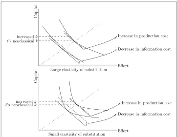
Fig. 4Input mix distortions and information rents as functions of the elasticity of substitution
the elasticity of substitution is large. In the bottom panel, the reduction in information rents is large when the elasticity of substitution is small. As a consequence of this rela-tionship, as the elasticity of substitution approaches zero, the quantity produced under the optimal restrictive contract approaches the first-best quantity, while the distortion in the capital-effort ratio goes to zero. It follows that fornsufficiently large, the optimal restrictive contract will generate greater total surplus than the optimal basic contract.
Matters are less straightforward when the two inputs are close substitutes. First (as in Fig. 3), an interior solution may exist but the determinant of the Hessian of the Lagrangian may be negative for sufficiently largeγ (see (14)). In this case, none of the machinery on which Proposition 7 is based can be applied. Second, suppose, for a sequence(gn) satisfy-ing A1–A3 withσ(¯ gn)increasing without bound, that an interior solution does exist and
the determinant of the Hessian of the Lagrangian is positive on [ 0, ]. In this case, both the input mix and output effects will converge to zero and there is no guarantee that the latter effect will dominate the former. Hence, it is possible that when the two inputs are close substitutes, the optimal basic contract yields a higher level of total surplus than the optimal restrictive contract. Finally, an interior solution for the restrictive contract may not exist. Specifically, ifθhwas slightly higher than the value represented in Fig. 3, then typehwould be able to imitatewithout utilizing any effort at all.
Conclusions
asymmetric information. Farmers’ private information regarding their productivity allows some farmers to collect information rents at the expense of the buyer. Restricting farmers’ scope for making production decisions can reduce those information rents and increase the buyer’s returns. The net effect on total surplus is indeterminate. Output is higher when the buyer controls the input, due to lower information rents accruing to more pro-ductive farmers. However, this reduction distorts input use away from the production cost-minimizing level, which is costly. The net effect on total surplus depends primarily on the elasticity of substitution between inputs. The less substitutability between labor and other inputs, the smaller the profit-maximizing distortion in the input ratio, and the smaller the reduction in the output specified in the contract for the low-ability agent. Both of these effects increase total surplus. Given the limited substitutability between labor and non-labor inputs in many agricultural activities, the analysis suggests that greater control of non-labor inputs by the buyer increases total surplus.
These findings have important implications relating to the design and welfare effects of agricultural contracts. Natural illustrations of inputs for which labor has limited substi-tutability are seeds supplied for the production of specialty crops and animals supplied by the buyer. In such cases, when the elasticity of substitution is low, our analysis implies that buyer control of inputs increases total surplus, even though it decreases the information rents obtained by some farmers.
Of course, there are other cases in which the elasticity of substitution may be high; for example, labor may substitute reasonably well for specific production techniques. In such instances, it is unclear whether total surplus is higher when the buyer requires specific production techniques or when the farmer chooses them. Importantly, regardless of the effect on total surplus, in either case the information rents accruing to some farmers will decline and returns to the buyer will increase. Consequently, our analysis contributes to the property rights literature by providing a strong argument for integration; the buyer’s profits are higher when she controls material inputs than when she does not in this framework.
Oftentimes in agricultural markets, buyers who contract with farmers have oligopoly power in their output markets. The effect identified in our model is not eliminated when oligopoly power is introduced by allowing the buyer to face a downward-sloping demand curve rather than a constant output price. The logic is simple. First, consider a buyer who is a monopolist in her output market. She will maximize expected profits, recognizing that marginal revenue is less than price. Exercising market power, her contract menu will specify lower outputs for farmers of each type. As a result, production and information costs will be correspondingly lower. The high ability farmer will still obtain information rents—i.e., the buyer will incur information costs—although these will be smaller in mag-nitude than in the perfectly competitive case. Moreover, the high ability farmer will still obtain a lower information rent under the restrictive contract than under the basic one. In summary, the presence of monopoly power does not eliminate the problem analyzed in this paper.
to negotiate a share of the buyer’s rents from the output market. Third, in contrast to Krattenmaker and Salop (1986), our buyer does not have the opportunity to increase her input purchases and output sales by contracting with additional farmers. This elim-inates another motivation—raising competitors’ costs —for contracting in an oligopoly. Once again, quantity is the only strategic variable available to the buyer in the context of our model structure, and the presence of market power will affect contract menu design only through its effect on this variable. Thus, the insights of the analysis can be applied to questions regarding agricultural contracts even in markets where buyers have market power.
The results of the analysis provide a way of evaluating the effects of government poli-cies regarding agricultural production contracts. Under pressure from farmers, Iowa and other US states enacted laws that banned meatpacker ownership or control of cattle and hogs intended for slaughter. While contracting per se was not outlawed under these mea-sures, contracts where the meatpacker controls major production decisions were. In our context, the laws outlawed restrictive contracts in which the meatpacker specifies non-labor inputs but did not outlaw basic contracts in which the farmer chooses the means of production (McEowen et al. 2002). Clearly, the reduced information rents farmers receive under integration and input control contracts provided them with an incentive to lobby for these laws. Our framework allows us to assess the social desirability of such laws. Because labor has a limited ability to substitute for animals in meat production, this type of contract provisions almost certainly do not increase total surplus in our frame-work. They can only promote efficiency if another market failure exists and its effects are mitigated by replacing the spot market with contracted and integrated production. On the other hand, the substitutability of labor for specific production techniques may be somewhat higher, so that the efficiency implications of such contract provisions are less clear.
In Iowa, major processors sued the state government, arguing that the ban was uncon-stitutional. The state settled with the companies starting in 2005 and continuing through 2013. The settlement agreements addressed concerns outside our modeling framework that could affect returns to farmers, including retaliation against contracting farmers who formed or joined a contract grower’s association and transparency regarding the data used to calculate compensation, among other considerations. It also allowed the proces-sors to continue to use contracts (Iowa Department of Justice 2013). Our analysis suggests that the settlements will promote efficiency, provided that the elasticity of substitution between farmers’ labor and inputs specified in the production contracts is sufficiently low.
Endnotes
1Unlike production contracts, marketing contracts only address the product at the time
of delivery, including the pricing mechanism, delivery time and location, and verifiable product characteristics.
2In turn, most of these provisions (94 %) linked compensation to the grower’s
3Recent discussions of other aspects of the contracting literature and of issues related to
analyzing agricultural contracts include Goodhue (2011), Sexton (2013), and Wu (2014).
4Assumptions A1 and A2 are much stronger than we need, but the computational
convenience that these assumptions provide amply compensates for the loss of generality.
5Becausef is homogeneous of degreeα (A2),f¨(e¨(q,θ),θ) = ¨e(q,θ)αf(1,β˜,θ) =
¨ e(q,θ)α
˜
e(q,θ)−αf
˜
e(q,θ),k˜(q,θ)
= f
˜
e(q,θ),k˜(q,θ)
.
6From the buyer’s perspective, the farmer’s information rents are a cost.
7For reasons that will become clear, typehis in the numerator of but the
denomina-tor of = θθh (p. 6).
8To see why inequality (8) holds, suppose first that k = ˜k(q,θ). In this case,
¯
CI(q,k)= ¯CP(q,k)− ¯ChP(q,k) is the difference between the two type’s production costs, when typehis constrained to use the same level of capital as type. But since this level is super-optimal forhfor producingq, the cost differenceC˜I(q)= ˜CP
(q)− ˜ChP(q), whenh
is permitted to substitute labor for capital, is even greater. Ifk >k˜(q,θ), thenkwould be even more super-optimal forhfor producingq, and hence the gain tohfrom replac-ing surplus capital with labor would be even higher. Figure 1 illustrates this argument graphically.
9Figure 2 makes clear that neither A1 or A2 is required for this result to hold. A
suf-ficient but still far from necessary condition is that the difference between types be technologically neutral, in the sense that for anyq, the isoquants associated with thatq for the two types be parallel to each other.
10The elasticity of substitution off at(e,k)is denoted by (see Silberberg (1990))
σke(e,k)= −∂
ln(k/e) ∂ln(fk/fe)
f(e,k)=constant= − d(fk/fe)
fk/fe
d(k/e)
k/e f(e,k)=constant = − fefk(fee+fkk)
ek (fk)2fee−2fefkfek+(fe)2fkk
!.
11Because the buyer has only one choice variable under a basic contract, there is no
need to set up a Lagrangian corresponding to (10) to determine the cost function.
Appendix Proof of Lemma 1:
The optimal restrictive contract is the solution to the following program:
max (q¯,k¯,¯t)
i∈{,h}
φipq¯(θi)− ¯t(θi) (22a)
subject to ¯t(θ) ≥ C¯P(q¯(θ),k¯(θ),θ) (22b) ¯
t(θh) ≥ C¯P(q¯(θh),k¯(θh),θh) (22c) ¯
t(θ) − C¯P(q¯(θ),k¯(θ),θ) ≥ ¯t(θh) − C¯P(q¯(θh),k¯(θh),θ) (22d) ¯
t(θh) − C¯P(q¯(θh),k¯(θh),θh) ≥ ¯t(θ) − C¯P(q¯(θ),k¯(θ),θh). (22e)
Now, given(q¯,k¯,¯t)define theinformation rent vectordt¯ by forθ ∈θ,θh,dt¯(θ) = ¯