Copyright © 2012 CTTS.IN, All right reserved
Computation of All Stabilizing PID Controllers for
High-Order Systems with Time Delay in a Graphical Approach
Seyed Zeinolabedin Moussavi
Designation : PhD of Control Engineering, Organization : Faculty of Electrical Engineering, Shahid Rajaee Teacher Training University, Email ID : [email protected]
Hassan Farokhi Moghadam
Designation : M.Sc Student of Control Engineering, Organization : Faculty of Electrical Engineering, Shahid Rajaee Teacher Training University, Email ID : [email protected]
Abstract — In the present paper, the problem of computation of all stabilizing high-order time delay systems using well known and efficient proportional-integral-derivative (PID) controller is investigated in a graphical approach. An efficient approach to this important problem is presented. Based on this approach, all PID controllers that will ensure stability are determined in a
(
k
p,
k
i,
k
d)
plane and then the stability boundary in a(
k
i,
k
d)
plane for a constant value ofk
p is determined and analytically described. It is shown that the stabilizing(
k
i,
k
d)
plane consists of triangular regions. The generalized Hermite-Biehler theorem which is applicable to quasipolynomials and finite root boundaries which will be described in detail in continuation are studied to establish results for this design and also determining region of stability of designed PID controllers. Bode diagram criterion is used to show the stabilizing PID gain and phase margins. Step response is also used to show the correctness and advantage of the approach in two examples which are given to illustrate the method.Keyword — High-order systems, PID controller, Stabilizing regions, Time-delay.
1. I
NTRODUCTIONTime delay is the time for system to answer a specific command after exerting an input. It can be also defined as the required time between applying change in the input and notices its effect on the system output. Delay can be seen in most of systems and its effects are considered in synthesis and analysis of systems. Delays are often causes for instability and poor performance of system and make stability analysis and controller design difficult.
Most of classical methods used for controller design cannot be used with delayed systems. This is due to the
fact that the system’s future behaviors depend not only on
the current value of the state variables, but also some past history of the state variables.
In last decades widespread studies over time delay systems have been done. Main reasons for this development can be stated as follows [1]:
I. Delays are frequently used to simplify high-order models.
II. It can be shown that delay in difference equations can be achieved partially easy by simplification of system model.
On the other hand, PID controllers are used frequently in various engineering applications. Due to this comprehensive use of PID controllers in industrial and applications, a significant effort has been done to determine the set of all PID controllers that meet specific design goals [2]. The design was done by Ziegler and Nichols [3] for the first time and many formulas and equations have been extracted for different proposed design methods after the publication of the first design [4].
In attention to the great industrial use of this kind of controller and also the point that time delays are usually unavoidable in many mechanical and electrical systems, we can claim that even a partial improvement in PID design can be theoretically or practically effective and useful.
For this great controller many design methodologies have been studied and made. For example, in [5], the D-decomposition approach has been used to determine the stabilizing region of PID controllers. A characterization of all stabilizing PID controllers for an arbitrary plant in a computational way has been proposed in [6]. In [7], a parametric Kharitonov region for the PID controllers to guarantee stability and robustness has been proposed. A generalization of the Hermite–Biehler theorem has been used for determining the stabilizing PID controller based on the inverse Nyquist plot in [8]. The [9] computes the stabilizing PI and PID controllers to achieve gain and phase margins for processes with time delay.
Recently, the problem of finding the stabilizing PID controllers for high-order delayed systems positive or negative, has been studied in [10]. Nyquist criterion is another subject in dealing with high-order unstable delayed plants which were studied in [11].
high-Copyright © 2012 CTTS.IN, All right reserved order time delay systems based on generalization of the
Hermite-Biehler theorem is presented in a graphical approach. We also use the theorem of finite root boundaries which will be described in the next section to get better results by which the region of stability is determined and also plotted.
Bode plot is used to show the stabilizing PID gain and phase margins in the illustrative examples.
It's worthy to note that step response plot is also used to show the correctness of our proposed stabilizing method. The organization of this paper is as follows: In Section 2, the problem is stated. We also state a definition and also two important theorems which help us with getting desired and trustworthy results. Section 3 shows stabilization using a PID controller method. In this section our approach of design is explained clearly and all stabilizing PID parameters are determined. Section 4 shows illustrating of the approach by two examples which will be analyzed by MATLAB and simulation results will show the advantages of this approach. Finally, in section 5, the main conclusions are summarized.
2. P
ROBLEMF
ORMULATIONA
NDP
RELIMINARIESPID is a combination of three controllers: proportional, derivative and integral controller. One of the main interesting features of PID controllers is their simplicity. The most general form of then is the second order system in the s-domain defined as follows:
.
)
(
k
s
s
k
k
s
K
i dp
(1)We consider in this sectionG( s)as the transfer function of high-order time delay systems defined by.
sn n n n
m m m m
s
e
s
s
s
s
s
s
e
s
D
s
N
s
G
0 1 1
1
0 1 1
1
...
...
)
(
)
(
)
(
(2)
The degree of the denominator is higher than that of the numerator in this representation. Equivalently it would be strictly proper, and
n
m
2
in this study.Fig.1. Unity feedback control system.
The goal in this computations is to find the regions in terms of kp, ki , and kd such that the closed loop characteristic polynomial of the system in fig 1 be Hurwitz stable.
The characteristic polynomial is written as
)
(
)
(
1
)
(
s
K
s
G
s
(3)Let
s
j
, So)
(
)
(
1
)
(
j
K
j
G
j
(4)Definition 1 [8,12]. Let
(
s
)
(
s
2)
s
(
s
2)
o e
be agiven real polynomial of degree n, where
e(
s
2)
and)
(
s
2s
o are the components of
(s
)
made up of even and odd powers of s, respectively.Definition 2 [13]. A finite root boundary in the
k ,
dk
i
plane for a constant value ofk
p is the locus, wherecharacteristic function of fig 1 has a root
s
j
on theimaginary axis with a finite
R
. If0, the rootboundary is called a real root boundary (RRB) and when0, it's a complex root boundary (CRB). If the
root boundary is crossed from its unstable side, the corresponding root moves from the right half plane (RHP) to the LHP.
Theorem 1 [8,12].
Let
(
s
)
0
1s
...
ns
n be a given realpolynomial of degree n, numbers of roots of
(s
)
inleft-half plane and right-left-half plane, are denoted by
l
andr
respectively, and
(
)
l
r
. Then),
(
2
))
(
(
0
j
where
.
)
(
))
(
(
0
0
j
j
d
)
(
)
(
j
This is called "Generalization of the Hermite-Biehler
Theorem". Theorem 2 [13]
Given a delayed system with the (2) and a f()kp
fulfilling the conditions in Definition 2, the finite root boundaries in the
k ,d ki
plane for a fixed value of kpare the following lines
I.
k
i
0
,
if
a
0
0
andk
p
f
0(RRB),II.
k
i
0
,
if
a
0
0
andk
p
f
0(RRB),III.
k
i
2k
d
g
(
)
for all
(CRB)IV.
k
i
2k
d
g
(
)
for all
(CRB)with
(
)
sin(
)
(
)
cos(
)
)
(
f
2L
f
1L
g
)
(
lim
00
f
f
, which exists fora
0
0
.
Copyright © 2012 CTTS.IN, All right reserved All of these theorems and preliminaries are used in
getting better results which are shown in coming examples for instance.
3. A
LLS
TABILIZINGPID C
ONTROLLERSThe stabilizing techniques used in this paper are based on decomposing the delayed system into real and imaginary parts and then using theorems and definitions in previous section. It can result in graphical method which is capable of ensuring closed loop stability of system.
The following four steps are proposed to find the boundaries of a PID controller that ensure the stability.
I. Decompose the frequency form of the system without delay into real and imaginary parts, and substitute them into (15)-(16) to obtain the PID parameters.
II. Analyze the system in presence of time delay, and redo the procedures.
III. Determine the PID stability boundaries of the system using their related equations in this section and theorems 1 and 2.
IV. Finally, plot the all stabilizing regions and then
i
k
versusk
d for a stabilizing constant value ofp
k
.This approach is used in our example and the results show the advantages of it in the next section.
Now the following equations are represented in the frequency domain.
))
(
Im(
))
(
Re(
)
(
j
G
j
j
G
j
G
(5)
Re(
(
))
Im(
(
))
)
(
1
)
(
j
G
j
j
G
k
k
j
k
j
i d p (6)By expanding
(
j
)
into real and imaginary parts, (6) can be written as)
(
)
(
)
(
j
R
j
jI
j
(7)where
d i pk
j
G
k
j
G
k
j
G
j
R
2))
(
Im(
))
(
Im(
))
(
Re(
)
(
(8)
di p
k
j
G
k
j
G
k
j
G
j
I
))
(
Re(
))
(
Re(
))
(
Im(
)
(
2
(9)Now all stabilizing regions can be determined like what is shown in "figs" 2 and 5. Note that we complete the calculations here just for a constant value of
k
d in the
k ,
pk
i
plane, for brevity. The other cases are obtained similarly. Of course they can be seen in our example results completely. Looking through the frequency-domain form of PID controller in (6), it is clear thatk
iand
k
d are at the imaginary part and they would be depend on each other. Of course this point is clear incoming equations and using theorems 1 and 2 help us in determining stabilizing regions.
By putting (8)-(9) equal to zero, we have
,
0
)
(
0
)
(
j
I
j
R
(10)which results in
2
)
(
)
(
Re
)
(
j
G
j
G
k
p (11)and
2 2)
(
)
(
Im
)
(
j
G
j
G
k
k
i d (12)where
2 2
2
)
(
Im
)
(
Re
)
(
j
G
j
G
j
G
(13)It can be written that
(
)
sin
)
(
)
(
Im
,
)
(
cos
)
(
)
(
Re
j
G
j
G
j
G
j
G
(14)where
(
)
G
(
j
)
.Therefore, (11) ad (12) can be simplified as
)
(
)
(
cos
)
(
j
G
k
p (15)and
)
(
)
(
sin
)
(
2
j
G
k
k
i d (16)Although it's somewhat similar to the way used in [9], but the final equations in (15) and (16) are main concerns here which have not been considered in [9]. Based on these equations, it can be claimed that the
k
p only affectsthe odd frequencies of the roots of (5), whereas the even frequencies of roots of (5) are influenced by
k
i andk
d.Now all the stabilizing boundary for
(
k
p,
k
i,
k
d)
isdetermined first and then
k
i versusk
d is plotted basedon theorem 2 for a constant value of
k
p in its stabilizing boundary. Bode plot can be used for determining stabilizing gain and phase margins in this condition. According to Theorem 1, when designed PID controller makes system stable, numbers of roots of
(s
)
in left-half plane are equal with degree real of polynomial)
(
l
n
and there be no number of roots of
(s
)
inright-half plane
(
r
0
)
.Copyright © 2012 CTTS.IN, All right reserved D
r
and also some roots in left-half plane which we call theml
D, in this paper. By simplifyingG
(s
)
into (15)-(16), according to theorem 1 there should be at leastD D
l
r
n
roots in left-half plane. Now, Stability conditions and then the stability regions can be obtained. This approach is illustrated by examples in the next section.4. I
LLUSTRATIVEE
XAMPLESExample 1:
In this example we consider a third order unstable transfer function time delay system
s
e
s
s
G
3 0.5)
1
(
1
)
(
which has been analyzed in [5].
At first the region of stability of
k
p is determined. Using Theorems and explanations in the previous sections, system is unstable in the intervals of(-
0.852)
and)
37
.
5
(
. As a great result, the possible stabilizingregion of
k
pis the interval(-
0
.
852
5.37
)
.Therefore, all stabilizing regions for the PID controller are shown in fig 2.
Now we choose a fixed
k
p in this region and thendetermine the stabilizing region of
k
i andk
d and this region is plotted and shown in fig 3.Now after determining the stabilizing boundary of different controllers of PID, the step response of the closed loop system is plotted for a special case,
3.189
,
186
.
1
,
1
d ip
k
k
k
. From fig 4, we cansee that the closed-loop system is stable. According to fig
5, stabilizing phase margin is obtained
49
.
5
atfrequency
sec
rad
0.468
, which can be concluded as a greatresult. Gain margin is also
7
.
35
dB
at frequencysec
rad
2.36
which is another good factor for this design.Fig.2. All stabilizing boundaries of the PID controller.
Fig.3. Stability boundaries in the
(
k
i,
k
d)
plane for1
pk
.0 5 10 15 20 25 30 35 40 45
0 0.2 0.4 0.6 0.8 1
1.2 Step Response
Time(sec)
Am
pl
itu
de
Copyright © 2012 CTTS.IN, All right reserved -100
-50 0 50
M
ag
nit
ud
e
(d
B)
10-2 10-1 100 101 102 0
90 180 270 360
Ph
as
e
(d
eg
)
Bode Diagram
Frequency (rad/s)
Fig.5. Bode diagram of the system at example 1.
Example 2:
In this example we consider one form of high-order transfer function which has been considered in [14], as follows:
s
e
s
s
s
G
3 0.1)
1
2
.
0
)(
1
4
(
1
)
(
Again we want to find all stabilizing PID controllers so that the closed loop system would be stable.
Using (15), theorems 1 and 2 we obtain the stabilizing interval of
k
p. Therefore, system is unstable in thek
p-intervals of
(-
1.12)
and(19.2
)
. As a greatresult, the possible stabilizing region of
k
p is theinterval
(
1
.
12
19.2
)
.In other words, the imaginary part
(s
)
has only simplereal roots if and only if
k
p
(-
0
.
852
5.37
)
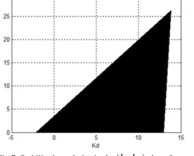
.All stabilizing regions for the PID controller are shown in fig 6.
Now we choose
k
p
5
which is in this region and thenthe stabilizing region of
k
i andk
d is determined and this region is plotted and shown in fig 7.Here in this special case, the PID controller parameters and transfer function are
3.84
,
6.25
,
5
d ip
k
k
k
)
814
.
1
1314
.
3
(
2
)
(
j
j
K
It can be written that the PID controllers that ensure stability in the
(
k
i,
k
d)
plane for a constant value ofk
phave been determined in a well defined set and region. In
this example, we have considered
k
p
5
which is in the stability boundary obtained in previous computations. By determining the possible stabilizing region, we plot the step response of the closed loop system in fig 8 to show the stability.Bode diagram for closed-loop system is shown in fig 9 which illustrates that stabilizing gain and phase margin are achieved and the design procedure and evaluation are ended.
According to this fig, we can see that desired phase
margin (
54
.
3
) at frequencysec
rad
2.79
, has beenachieved. Gain margin is also
5
.
89
dB
at frequencysec
rad
5.24
.Fig.6. All stabilizing regions for the PID controller.
Fig.7. Stability boundaries in the
(
k
i,
k
d)
plane for5
pCopyright © 2012 CTTS.IN, All right reserved
0 5 10 15 20 25
0 0.2 0.4 0.6 0.8 1 1.2
1.4 Step Response
Time(sec)
Am
pl
itu
de
Fig.8. Closed-loop step response for example 2.
-150 -100 -50 0 50 100
Ma
gn
itu
de
(d
B)
10-2 10-1 100 101 102 103 -90
0 90 180 270
Ph
as
e (
de
g)
Bode Diagram
Frequency (rad/s)
Fig.9. Bode diagram for closed-loop system of second example.
5. C
ONCLUSIONIn this paper, we presented a graphical approach to design all stabilizing PID controllers for high-order systems with time delays. It provides an efficient and straightforward method for stabilization of PID controller. We could obtain all stabilizing PID controller in
(
k
p,
k
i,
k
d)
plane and also the stabilizing regions of)
,
(
k
ik
d for a fixed value ofk
p, as well. Avoiding complex mathematical derivations and good quality and efficiency are some advantages of this approach. Numerical examples with time delay were presented to demonstrate the effectiveness of this method.R
EFERENCE[1] J. P. Richard, Time delay systems: An overview of some recent advances and open problems,
Automatica, vol. 39, pp. 1667-1694, 2003.
[2] T. Emami and J. M. Watkins, Robust Performance Characterization of PID Controllers in the Frequency Domain, WSEAS transactions on systems
and control, pp. 232-242, 2009.
[3] J.G. Ziegler and N.B. Nichols, Optimum settings for automatic controllers, Trans. ASME, vol. 64, pp. 759-768, 1942.
[4] Y-Y. Li, A-D. Sheng, Y.G. Wang, Synthesis of PID-type controllers without parametric models: A graphical approach, Energy Conversion and Management 49, pp. 2392-2402, 2008.
[5] Y-Y Li, G-Q. Qi, A-D. Sheng, Frequency parameterization of H∞ PID controllers via relay
feedback: A graphical approach, Journal of Process
Control 21, pp. 448-461, 2001.
[6] M. T. Ho, A. Datta and S. P. Bhattacharyya, Generalizations of the Hermite–Biehler Theorem: The complex case, Linear Algebra and its Applications, pp. 23-36, 2000.
[7] Y.J. Huang, Y.J. Wang, Robust PID tuning strategy for uncertain plants based on the Kharitonov theorem, ISA Transactions 39, pp. 419-431, 2000. [8] B. Fang, Computation of stabilizing PID gain
regions based on the inverse Nyquist plot, Journal
of Process Control 20, pp. 1183-1187, 2010.
[9] N. Tan, Computation of stabilizing PI and PID controllers for processes with time delay, ISA
Transactions 44, pp. 213–223, 2005.
[10] D.J. Wang, Synthesis of PID controllers for high-order plants with time-delay, Journal of Process
Control 19, pp.1763-1768, 2009.
[11] S. Ch. Lee and Q-Guo Wang, Stabilization conditions for a class of unstable delay processes of higher order, Journal of the Taiwan Institute of
Chemical Engineers 41, pp. 440-445, 2010.
[12] M.T. Ho, A. Datta, S.P. Bhattacharyya, Generalizations of the Hermite-Biehler theorem,
Linear Algebra Appl. 302 and 303, pp. 135-153,
1999.
[13] N. Hohenbichler, All stabilizing PID controllers for time delay system, Automatica 45, pp. 2678-2684, 2009.