INTELIGENCIA ARTIFICIAL
http://journal.iberamia.org/
Effects of Dynamic Variable - Value Ordering
Heuristics on the Search Space of Sudoku Modeled
as a Constraint Satisfaction Problem
James L. Cox
[1], Stephen Lucci
[2], Tayfun Pay
[3] [1]Brooklyn College of New York 2900 Bedford Avenue
Brooklyn, NY 11210 [2]
The City College of New York 160 Convent Avenue
New York, NY 10031
[1,3]Graduate Center of New York
365 5thAvenue New York, NY 10016 [1]
[email protected] [2][email protected] [3]
Abstract We carry out a detailed analysis of the effects of different dynamic variable and value ordering heuristics on the search space of Sudoku when the encoding method and the filtering algorithm are fixed. Our study starts by examining lexicographical variable and value ordering and evaluates different combinations of dynamic variable and value ordering heuristics. We eventually build up to a dynamic variable ordering heuristic that has two rounds of tie-breakers, where the second tie-breaker is a dynamic value ordering heuristic. We show that our method that uses this interlinked heuristic outperforms the previously studied ones with the same experimental setup. Overall, we conclude that constructing insightful dynamic variable ordering heuristics that also utilize a dynamic value ordering heuristic in their decision making process could improve the search effort for some NP-Complete problems.
Keywords: Backtracking-Search, Constraint Satisfaction Problems, Dynamic Variable Ordering Heuristics, NP-Completeness, Phase-Transition, Sudoku
1
Introduction
The manner in which the search space of a problem that has been modeled as a CSP (Constraint Satis-faction Problem) is explored depends on the various techniques that are built into the given CSP solver. These techniques might include filtering algorithms such as arc-consistency and path-consistency, random-restarts, back-jumping as well as dynamic variable ordering and dynamic value ordering heuristics.0 All of these methods are important in their own right, but dynamic variable ordering and dynamic value ordering heuristics are especially important since they guide the backtracking search. In other words, combination of these heuristics could choose a variable and value pair that direct the search along a path
ISSN: 1137-3601 (print), 1988-3064 (on-line) c
where it is hard to recognize that no solution exists. Therefore, it is very important that these heuristics choose a variable and value pair that is more likely to either, direct the search along a path that is easy to determine that no solution exists, or direct the search along a path where a solution exists.
The study of dynamic variable ordering heuristics began with the dom heuristic of [3] that picks the next variable with the smallest domain size. A tie-breaker was introduced for the dom heuristic in [4] that breaks ties by picking the next variable with the highest initial degree, the number of unassigned neighbors. A more sophisticated version of this heuristic was already in use for graph coloring [5]. This heuristic breaks ties for the dom heuristic by picking the next variable with the current highest degree.1 A variant of this heuristic was proposed in [6], where the next variable with the minimum value of current domain size over current degree is selected. This heuristic works well for instances where the variables have wide range of degree in combination with small variance in their domain sizes, since dom/deg gives equal importance to domain size and degree. On the other hand, there has not been much attention given to dynamic value ordering. The most prominent work on this front was the lvo heuristics of [4] with four different ranking functions that employ forward-checking.
In this paper, we investigate various dynamic variable and value ordering heuristics with respect to Sudoku modeled as a CSP. Sudoku was first studied as a CSP in [7] and has been been getting a lot of attention in this field since then [8, 9, 10, 11, 12, 13], because it is a highly constrained challenging combinatorial search problem. We generated numerous Sudoku puzzles of size 16 by 16 (order-4), 25 by 25 (order-5) and 36 by 36 (order-6) using the setup outlined in [9]. We encoded the Sudoku puzzles as a CSP using the modeling technique from [11, 12] and also employed their arc-consistency algorithm. We observed the mean depth, mean number of explored variables and mean number of instantiations within a fixed time as well as the percentage of solved puzzles and mean time. We did this for seven different heuristics, including dom [3], an interpretation of dom+deg [5] and sd-lrv-mfv [11]. We refrained from investigating dom/deg [6]heuristic since it was already shown to not perform well for multiple permutation problems such as Latin Squares in [14] and Sudoku in [11].
We showed that lexicographically choosing the next variable performs better than randomly choosing the next variable. We demonstrated that using a dynamic variable ordering heuristic performs better than either randomly or lexicographically selecting the next variable. We also showed that the width of the search tree decreased when the dynamic variable ordering heuristic was used, which agrees with the results in [3, 15] and [16]. We demonstrated that adding a dynamic value ordering heuristic on top of a dynamic variable ordering heuristic does not necessarily improve the search effort, but instead adding a tie-breaker for the dynamic variable ordering heuristic does in fact improve the search effort. We showed that combining a dynamic value ordering heuristic with a dynamic variable ordering heuristic, that already utilizes a tie-breaker, might actually hinder the performance. We demonstrated that adding a dynamic value ordering heuristic as a second round of tie-breaker for the dynamic variable ordering heuristic enhances the search effort. We also detected the easy-hard-easy “phase-transition” as was previously observed with Sudoku puzzles in [9, 11, 12] and [13]. This is a phenomenon with all NP-Complete problems.
As far as we know, there has been no dynamic variable ordering heuristic that utilizes a dynamic value ordering heuristic as a tie-breaker, of course other than the ones introduced in [11]. Our experiments showed that even if we use a well-known dynamic variable ordering heuristic that employs a tie-breaker, such as dom+deg, that there could still be more ties and employing a dynamic value ordering heuristic as a second round of tie-breaker has a positive affect in the outcome of the search effort. Overall, we demonstrated that coming up with insightful dynamic variable ordering heuristics that also use dynamic value ordering heuristic in their decision making process, can help to guide the search effort for some NP-Complete problems. In fact, the performance achieved at the critical point by our most sophisti-cated heuristic is far better than the performance of the methods utilized in [9] and [13] with the same experimental setup.
0An excellent resource for most of these CSP techniques and many more is [1]. An excellent introduction written in Spanish is [2].
2
Methods
2.1
Encoding
We encode the Sudoku puzzles as a constraint satisfaction problem by using the natural combined model from [11, 12].
2.1.1 Natural Combined Model
The Sudoku puzzle is formulated on a 3DS(k∗k)∗(k∗k)∗(k∗k) Boolean matrix, wheren= (k∗k). We say that a Sudoku puzzle of orderkis annbynSudoku puzzle.
The primal variablexi,j is represented by the slice{S(i, j, v)|1≤v≤n}. The initial domain of xi,j
is denoted D(xi,j) and is{v|S(i, j, v) =T rue,1≤v≤n}.
The box dual variablebv,p,q wheredi/ke=p,dj/ke=qis represented by the slice{S(i, j, v)|((p−1)∗
k+ 1)≤i≤p∗k,((q−1)∗k+ 1)≤j≤q∗k}. The initial domain ofbv,p,q is denotedD(bv,p,q) and, is
{i, j|S(i, j, v) =T rue,((p−1)∗k+ 1)≤i≤p∗k,((q−1)∗k+ 1)≤j≤q∗k}.
The column dual variablecv,j is represented by the slice{S(i, j, v)|1≤i≤n}. The initial domain of
cv,j is denotedD(cv,j) and is{i|S(i, j, v) =T rue,1≤i≤n}.
The row dual variablerv,iis represented by the slice{S(i, j, v)|1≤j≤n}. The initial domain ofrv,j
is denoted D(rv,j) and is{j|S(i, j, v) =T rue,1≤j ≤n}.
Then the6= constraints are enforced as follows: 1) on pairs of primal variables within each box, column and row. 2) on pairs of box dual variables of each value. 3) on pairs of column dual variables of each value. 4) on pairs of row dual variables of each value.
2.2
Filtering Algorithms
The following filtering algorithms were introduced in [11, 12] and work together with the natural combined model. Although the backtracking-search is being conducted on the primal variables, consistency checks on the other three view-points of the problem are performed whenever deemed necessary.
2.2.1 Redundantly Modeled Forward Checking Algorithm (RFC)
The RFC algorithm verifies whether or not assigning a value to a variable is consistent with respect to it’s constraints. It also modifies the domains of the constrained variables accordingly. These checks and modifications are performed with respect to primal variables as well as the box, column and row dual variables.
Algorithm 1Redundantly Modeled Forward Checking
Input: (S, n, i, j, v)2
Output: Is {S(i, j, v) == True}consistent? 1: Stemp←S
2: if (Remove-All-Except-v== True) then
3: if (Remove-All-Other-v== True) then
4: S ←Stemp
5: returnTrue 6: end if
7: end if
8: returnFalse
9: functionRemove-All-Except-V
10: fork= 1...ndo
11: if (Stemp(i, j, k) == True ∧k6=v)then
12: if (Exists-In-Box(i, j, k) == False)then
15: if (Exists-In-Col(i, j, k) == False) then
16: returnFalse 17: end if
18: if (Exists-In-Row(i, j, k) == False)then
19: returnFalse 20: end if
21: Stemp(i, j, k)←False
22: end if
23: end for
24: returnTrue 25: end function
26: functionExists-In-Row(p, q, r) 27: fork= 1...ndo
28: if (Stemp(p, k, r) == True ∧k6=q)then
29: returnTrue 30: end if
31: end for
32: returnFalse 33: end function3
34: functionRemove-All-Other-V
35: if (Remove-V-From-Box== False)then
36: returnFalse 37: end if
38: if (Remove-V-From-Col== False)then
39: returnFalse 40: end if
41: if (Remove-V-From-Row== False)then
42: returnFalse 43: end if
44: returnTrue 45: end function
46: functionRemove-V-From-Row
47: fork= 1...ndo
48: if (Stemp(i, k, v) == True ∧k6=j)then
49: t←False
50: forl= 1...n do
51: if (Stemp(i, k, l) == True ∧l6=v)then
52: t←True
53: end if 54: end for
55: if t == Falsethen
56: returnFalse 57: end if
58: if (Exists-In-Box(i, k, v) == False)then
59: returnFalse 60: end if
61: if (Exists-In-Col(i, k, v) == False)then
62: returnFalse 63: end if
64: Stemp(i, k, v)←False
66: end for
67: returnTrue 68: end function4
2.2.2 Redundantly Modeled Arc-Consistency Algorithm One (RAC-1)
The RAC-1 algorithm takes the RFC algorithm one step further. Instead of just examining the constrained primal and dual variables of the instantiated variable, it checks all of the primal as well as all of the dual variables. It then verifies that they are consistent with the given assignment. Furthermore, it performs instantiations whenever the domain of some primal or dual variable becomes singleton, which forces it to repeat the whole process again. If the RAC-1 algorithm successfully executes, that is without finding an inconsistency, then the given puzzle is arc-consistent with respect to the primal and the box, column and row dual variables.
Algorithm 2Redundantly Modeled Arc-Consistency One
Input: (S, n)5
Output: Is S arc-consistent? 1: Stemp←S
2: t←1
3: whilet6= 0do
4: t←0
5: if (Check-Primal-Variables== False)then
6: returnFalse 7: end if
8: if (Check-Box-Variables== False)then
9: returnFalse 10: end if
11: if (Check-Col-Variables== False)then
12: returnFalse 13: end if
14: if (Check-Row-Variables== False)then
15: returnFalse 16: end if
17: end while
18: S←Stemp
19: returnTrue
20: functionCheck-Primal-Variables
21: fori= 1...ndo
22: forj = 1...ndo
23: if Stemp(i, j,0) == 0then6
24: c←0
25: v←0
26: fork= 1...ndo
27: if Stemp(i, j, k) == Truethen
28: c←c+ 1
29: v←k
30: end if
31: end for
32: if c==0then
2S, n, i, j, vandS
tempare global variables and accessible by all functions. 3
Exists-In-Box(p, q, r) andExists-In-Col(p, q, r) functions behave similarly. 4
33: returnFalse 34: else if c==1then
35: if RFC(Stemp, n, i, j, v) == Truethen
36: t←1
37: else
38: returnFalse 39: end if
40: end if
41: end if
42: end for
43: end for
44: returnTrue 45: end function7
2.3
Search Heuristics
The following heuristics are utilized with respect to primal variables.
2.3.1 Heuristic-1 (RAN&LEX)
Randomly select the unassigned variable; and lexicographically select the values in its domain.
2.3.2 Heuristic-2 (LEX&LEX)
Lexicographically select the unassigned variable; and lexicographically select the values in its domain.
2.3.3 Heuristic-3 (SD&LEX)
Lexicographically select the unassigned variable with the smallest domain size; and lexicographically select the values in its domain.
2.3.4 Heuristic-4 (SD&MFV)
Lexicographically select the unassigned variable with the smallest domain size; and order the values in it’s domain that occur from most frequently to least frequently in the domains of all of the assigned variables.
2.3.5 Heuristic-5 (SD-LRV&LEX)
Among the variables with the smallest domain size, lexicographically select the variable that has the least number of fixed variables among those with which it shares a constraint; and lexicographically select the values in its domain.
2.3.6 Heuristic-6 (SD-LRV&MFV)
Among the variables with the smallest domain size, lexicographically select the variable that has the least number of fixed variables among those with which it shares a constraint; order the values in its domain that occur from most frequently to least frequently in the domains of all of the assigned variables.
5S, nandS
tempare global variables and accessible by all functions. 7
2.3.7 Heuristic-7 (SD-LRV-MFV&MFV)
Among the variables with the smallest domain size that also have the least number of fixed variables among those with which it shares a constraint, lexicographically select the one that contains a value in its domain that occurs the most frequent times in the domains of all of the assigned variables; order the values in its domain that occur from most frequently to least frequently in the domains of all of the assigned variables.
Heuristic-1 serves the purpose of understanding how the backtracking search performs when the next variable to be assigned is chosen uniformly at random. Heuristic-3 is clearly the dom heuristic of [3]. Heuristic-4 serves the purpose of understanding how a dynamic variable ordering heuristic works with no tie-breaker, but with a value ordering heuristic. Heuristic-5 can actually be viewed as an interpretation of the Brelaz (dom+deg) heuristic of [5]. Heuristic-6 serves the purpose of examining how a dynamic variable ordering heuristic that has a tie-breaker works with a value ordering heuristic.
We should also note that we did experiment with the opposite tie-breaker, as was done in [11], the most number of constrained variables (MRV) and the opposite dynamic value ordering heuristic, order the values in it’s domain that occur from least frequently to most frequently in the domains of all of the assigned variables (LFV). However, none of the three possible combinations of these tie-breakers (LRV and MRV) and dynamic value ordering heuristics (MFV and LFV) worked as well as Heuristic-7.
3
Experimental Setup
We implemented the modeling method, the filtering algorithm and the search heuristics in C++. Then we generated the test instances by following the methodology that was outlined in [9] for Sudoku puzzles. We first randomly filled 5%-25% percent of the empty puzzle board without invalidating the puzzle and then randomly chose one of our algorithms to complete the puzzle. We generated 100 fully solved Sudoku puzzles of order 4, 5 and 6, which correspond to 16 by 16, 25 by 25 and 36 by 36 size Sudoku puzzles, respectively.
Then we removed a cell from a given fully solved puzzle with probabilityp, wherep = 0 implies a fully solved puzzle andp= 1 implies an empty one. We did this for all of the 100 fully solved puzzles of order 4 and 5 for each probabilityp, from p= 0.05 throughp= 0.95 with 0.05 increments. We used the Mersenne Twister Pseudo-Random generator mt19937 in C++ for generating our random numbers, that were uniformly distributed between 0 and 1. A total of 1900 puzzles were generated for Sudoku puzzles of order 4 and 5. We only generated 100 Sudoku puzzles of order 6 at the hard region so that we can verify our observations carry over to larger puzzles.
All of the puzzles we generated are guaranteed to have a solution, but they can have more than one solution. It would take a tremendous amount of time to verify that each puzzle has a unique solution, because we would have to check the possibility of a solution at every single path. Furthermore, the puzzles become so sparse at higher probabilities that it is impossible to guarantee that they have a unique solution.
We set the time limit to 30 seconds for Sudoku puzzles of order 4 and to 360 seconds for Sudokdu puzzles of order 5 since these were the time limits used in [9] and [13]. We set the time limit to 720 seconds for Sudoku puzzles of order 6.
4
Empirical Analysis
4.1
Order 4 Puzzles
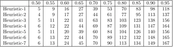
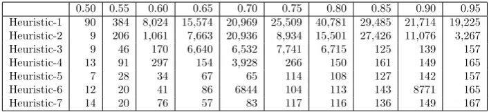
The performance of our seven heuristics when solving order 4 puzzles at different probabilities are pre-sented in tables 1 2 and 3 as well as in the corresponding graphs. The results of the methods in [9] and [13] are also included as graphs that show the percentage of solved puzzles at each probability versus mean time in seconds.
We observe that Heuristic-1 performed the worst with respect to being able to solve all of the instances at each probability within the allocated time. Heuristic-1 is followed by Heuristic-2 and Heuristic-3 where they also had an overall worse performance than the methods in [9] and [13]. However, when they were able to solve the given instances, they did so much faster than the methods in [9] and [13]. This can be seen in the corresponding graphs that show the mean time in seconds. On the other hand, Heuristic-5 and Heuristic-7 were able to solve all of the instances at each probability within the allocated time. And they did so in a very fast manner as can be seen by the corresponding graphs that show the mean time in seconds.
When a heuristic at some probability has the same or almost the same average depth, average number of explored nodes and average number of instantiations, it means that the search backtracked few times or it did not backtrack at all. This is the case at all of the probabilities for Heuristic-5 and Heuristic-7 and most of the probabilities for Heuristic-4 and Heuristic-6. The reason for this occurrence cannot really be attributed to the choice of a dynamic variable and value ordering heuristics, but it is due to the modeling choice as well as the constraint propagation algorithm that is being employed. In fact, the reason that the first three heuristics actually performed this well is due to this. In other words, the constraint propagation algorithm along with the encoding method overpowered the variable ordering aspect of our solver when solving order 4 puzzles.
Another observation is that the average number of instantiations that are roughly double the average number of explored nodes starting from Heuristic-3 and on. This is due to using the smallest domain heuristic in variable selection that allows the width of the search tree to be narrower and consequently results in a deeper search-tree. This observation concurs with the results in [3, 15] and [16] that the width of the search-tree decreases when the smallest domain heuristic is utilized. This difference will be more striking with order 5 puzzles.
4.2
Order 5 Puzzles
The performance of our seven heuristics when solving order 5 puzzles at different probabilities are pre-sented in tables 4 5 and 6 as well as in the corresponding graphs. The results of the methods in [9] and [13] are also included as graphs that show the percentage of solved puzzles at each probability versus mean time in seconds.
Heuristic-1 cannot solve any instances at probabilities 0.55, 0.6, 0.65 and 0.8 within the allocated time. Heuristic-2 performs some what better than Heuristic-1, but it still performs worse than the methods in [9] and [13]. On the other hand, the difference in performance between Heuristic-2 and Heuristic-3 is quite striking at each probability as can be observed from the corresponding graphs and tables. Heuristic-3 allowed the search effort to go further down in the search tree, which as a consequence resulted in more nodes being explored in the allocated time if no solution was found; or a solution was found with less number of explored nodes. This was also true with respect to the instantiations at each probability. As a result, the search was not stuck at a certain depth and more puzzles were solved at each probability within the given time limit. As we also observed with order-4 puzzles, the width of the search tree was minimized when Heuristic-3 was employed. This can be recognized with respect to the ratio between the average number of instantiations over the average number of explored nodes at each probability, which was approximately three with Heuristic-2 and two with Heuristic-3. This observation, once again, concurs with the results in [3, 15] and [16] that the width of the search-tree decreases when the smallest domain heuristic is utilized.
We observe from the corresponding graphs that Heuristic-5 significantly improved the search effort at the critical point of p= 0.55 compared to Heuristic-4 which performed similar to Heuristic-3. In fact, the difference of performance between Heuristic-3 and Heuristic-4 at the hard region was not statistically significant. This experiment distinguishes the importance of using a tie-breaker for the smallest domain heuristic over just coupling the smallest domain heuristic with a value ordering heuristic.
We also notice from the corresponding graphs that although Heuristic-6 performed a little better at the critical point of p = 0.55 compared to Heuristic-5, it actually performed worse at the subsequent probabilities of the heavy-tail region. This experiment demonstrates that adding value ordering heuristic without really gathering insight from the variable ordering heuristic does not necessarily yield better performance and it may actually hinder it.
As can be seen from the corresponding graphs, Heuristic-7 achieved a significant improvement over both Heuristic-5 and Heuristic-6. The performance at the critical point ofp= 0.55 is the most profound compared to the previous six heuristics. Heuristic-7, on average, was able to go further down in the search tree, traversed less number of nodes and made less number of instantiations. This demonstrates that a second round of tie-breaker for the smallest domain heuristic could be very useful. Indeed, the value ordering heuristic could be used for this purpose and it executes well for this intent. In other words, considering the values in the domains of the variables when breaking ties is relevant.
We also observe from the corresponding graphs that the methods in [9] and [13] did as well as our Heuristic-4 at the critical point ofp= 0.55 whereas our Heuristic-7 clearly out performed them at this significant point.
4.3
Order 6 puzzles
The performance of our seven heuristics when solving order 6 puzzles at the hard region are presented in table 7. We detect similar patterns with order 6 puzzles that we also observed with order 4 and 5 puzzles with respect to average depth, average nodes and average instantiations. However, this time the differences among the heuristics are more profound, because there are more unassigned variables with domain sizes that are greater than two and as a result, Heuristic-1 and Heuristic-2 perform even worse. Although Heuristic-3 and Heuristic-4 cannot solve any instances within the allocated time, they still perform better than Heuristic-1 and Heuristic-2 since they were able to go further down the search-tree and thus explored more nodes on average. Heuristic-7 solves the most instances and it is followed by Heuristic-6 and Heuristic-5. The performance of Heuristic-7 when solving order 6 puzzles at the hard region is further evidence that considering the values in the domains of the variables when selecting the next variable to instantiate does in fact make a difference in guiding the search effort.
0.50 0.55 0.60 0.65 0.70 0.75 0.80 0.85 0.90 0.95
Heuristic-1 5 9 16 27 39 53 70 83 98 118
Heuristic-2 4 9 17 27 44 61 77 95 113 137
Heuristic-3 5 11 22 41 63 83 103 123 138 156
Heuristic-4 6 12 22 44 69 87 109 131 147 164
Heuristic-5 5 11 20 39 60 84 104 126 140 156
Heuristic-6 6 13 22 44 70 89 112 132 148 165
Heuristic-7 6 13 24 45 70 90 113 134 149 167
Table 1: Average depth of the search tree at each probability for order 4 puzzles
0.50 0.55 0.60 0.65 0.70 0.75 0.80 0.85 0.90 0.95 Heuristic-1 28 160 2,273 4,269 5,609 7,020 11,222 8,493 5,897 5,328 Heuristic-2 6 87 442 2,339 6,825 3,267 5,471 9,774 4,065 1,482 Heuristic-3 6 27 94 3,338 3,295 3,897 3,403 124 138 156
Heuristic-4 9 50 158 97 1,997 175 129 145 148 164
Heuristic-5 5 18 25 52 62 98 105 126 140 156
Heuristic-6 9 16 30 64 3,436 96 112 137 4,431 165
Heuristic-7 9 16 49 50 76 102 114 135 149 167
0.50 0.55 0.60 0.65 0.70 0.75 0.80 0.85 0.90 0.95 Heuristic-1 90 384 8,024 15,574 20,969 25,509 40,781 29,485 21,714 19,225 Heuristic-2 9 206 1,061 7,663 20,936 8,934 15,501 27,426 11,076 3,267 Heuristic-3 9 46 170 6,640 6,532 7,741 6,715 125 139 157
Heuristic-4 13 91 297 154 3,928 266 150 161 149 165
Heuristic-5 7 28 34 67 65 114 108 127 142 157
Heuristic-6 12 20 41 86 6844 104 113 143 8771 165
Heuristic-7 14 20 76 57 83 117 116 136 149 167
Table 3: Average number of instantiations at each probability for order 4 puzzles
0.50 0.55 0.60 0.65 0.70 0.75 0.80 0.85 0.90 0.95 Heuristic-1 22 49 69 101 138 170 210 248 288 326 Heuristic-2 20 48 70 102 141 169 216 260 280 320 Heuristic-3 26 69 102 154 203 250 300 346 387 427 Heuristic-4 25 70 107 162 218 263 321 361 404 446 Heuristic-5 25 69 108 153 206 253 301 348 391 429 Heuristic-6 27 72 118 163 219 263 313 362 398 442 Heuristic-7 26 74 116 162 216 266 319 362 404 443
Table 4: Average depth of the search tree at each probability for order 5 puzzles
0.50 0.55 0.60 0.65 0.70 0.75 0.80 0.85 0.90 0.95
Heuristic-1 47,044 133,714 135,957 142,250 140,868 142,004 156,206 134,533 113,051 73,159 Heuristic-2 40,706 135,905 134,490 106,990 90,329 101,750 97,151 107,546 204,505 138,951 Heuristic-3 38,130 158,853 150,619 70,106 18,159 41,850 8,509 7,726 579 457 Heuristic-4 35,990 166,221 133,956 45,065 44,181 51,999 39,672 22,142 1,436 8,958 Heuristic-5 19,949 113,120 81,071 60,149 37,510 51,910 8,603 389 14,176 473 Heuristic-6 26,080 112,179 107,804 77,751 43,837 23,859 31,291 7,038 20,272 6,979 Heuristic-7 27,539 101,227 73,391 37,723 19,038 14,087 12,826 16,465 514 662
Table 5: Average number of explored nodes at each probability for order 5 puzzles
0.50 0.55 0.60 0.65 0.70 0.75 0.80 0.85 0.90 0.95
Heuristic-1 176,119 515,880 535,476 566,626 561,713 561,895 611,545 520,519 433,597 278,044 Heuristic-2 112,075 391,026 395,833 300,883 258,723 290,502 286,054 306,336 597,076 466,662 Heuristic-3 76,250 317,693 301,200 140,112 36209 85714 16741 15164 778 494 Heuristic-4 71,970 332,428 267,866 90,186 88,936 105,301 79,123 44,225 2,664 17,513 Heuristic-5 39,886 226,222 162,081 120,190 74,894 103,666 16,927 438 28,022 536 Heuristic-6 52,148 224,313 215,561 155,410 87,599 47,529 63,880 13,741 42,252 13,553 Heuristic-7 55,610 202,314 146,721 75,322 37,920 24,852 26,190 32,610 626 883
Table 6: Average number of instantiations at each probability for order 5 puzzles
Solved Avg. Time Avg. Depth Avg. Nodes Avg. Inst.
Heuristic-1 0% 720 secs 302 123,294 580,268
Heuristic-2 0% 720 secs 207 144,089 472,677
Heuristic-3 0% 720 secs 433 205,125 410,570
Heuristic-4 0% 720 secs 464 217,037 446,432
Heuristic-5 2% 691 secs 459 190,939 390,949
Heuristic-6 4% 677 secs 487 181,660 363,736
Heuristic-7 11% 623 secs 481 165,015 333,751
5
Conclusion
We conducted a detailed analysis of how dynamic variable and value ordering heuristics affect the search effort for Sudoku when the encoding method and the filtering algorithm are fixed. One of the most striking insights we gained from this experiment is the importance of incorporating a dynamic value ordering heuristic into the decision making process of a dynamic variable ordering heuristic. We observed that as the search space got smaller, there were still many more ties even after the first tie-breaker. If at this point the dynamic variable ordering heuristic makes a decision without considering the values in those variables domain, then it might very well go down a path where it is hard to recognize that no solution exists. However, by also considering the values in that variables domain, it can gain more insight on which path to guide the search. For instance, if there are some values that can only be fixed to few variables then it is better to guide the search with variables that have those values in their domains. So that we can either reach a solution faster or backtrack faster if it fails. Of course, this is especially true when the number of values in the domains of all the variables come from a discrete set of values, which is the case for Sudoku. However, we believe that the insights gained from this study can be carried over to other NP-Complete problems that are modeled as constraint satisfaction problems. This is because there are still many more ties left after applying a dynamic variable ordering heuristics and traditionally they are broken lexicographically without consulting any heuristic. We hope to further study the effects of dynamic variable and value ordering heuristics with more sophisticated constraint propagation algorithms.
References
[1] F. Rossi, P. van Beek, and T. Walsh. Handbook of constraint programming. Elsevier, 2006.
[2] F. Barber and M. A. Salido. Introduction to constraint programming.Inteligencia Artificial, Revista Iberoamericana de Inteligencia Artificial, 20:13–30, 2003.
[3] R. M. Haralick and G. L. Elliot. Increasing tree search efficiency for constraint satisfaction problems. Artificial Intelligence., 14:263–313, 1980.
[4] D. Frost and Dechter R. Look-ahead value ordering for constraint satisfaction problems. IJCAI95, pages 572–578, 1995.
[5] D. Brelaz. New methods to color the vertices of a graph. Communications of the ACM., pages 251–256, 1979.
[6] C. Bessiere and J.C. Regin. Mac and combined heuristics: Two reasons to forsake fc (and cbj?) on hard problems. CP96, pages 61–75, 1996.
[7] H. Simonis. Sudoku as a constraint problem. Workshop on Modelling and Reformulating Constraint Satisfaction Problems., pages 13–27, 2005.
[8] T. Cazenave. A search based sudoku solver. Labo IA Dept. Informatique Universite Paris, 2006.
[9] R. Lewis. Metaheuristics can solve sudoku puzzles. Journal of Heuristics., 13:387–401, 2007.
[10] L. Chaimowicz and M.C. Machado. Combining metaheuristics and csp algorithms to solve sudoku. Games and Digital Entertainment (SBGAMES), 2011 Brazilian Symposium on, pages 124–131, 2011.
[11] T. Pay. Some enhancement methods for backtracking-search in solving multiple permutation prob-lems. PhD Dissertation, Graduate Center of New York, CUNY., 2015.
[12] T. Pay and J. L. Cox. Encodings, consistency algorithms and dynamic variable-value ordering heuris-tics for multiple permutation problems. International Journal of Artificial Intelligence, 15(1):33–54, 2017.
[14] I. Dotu, A. Del Val, and M. Cebrian. Redundant modeling for the quasigroup completion problem. The International Conference on Principles and Practice of Constraint Programming -03., pages 288–302, 2003.
[15] B. M. Smith and S. A. Grant. Trying harder to fail first. Research Report Series-University of Leeds School of Computer Studies Lu Scs Rr, 1997.