R E S E A R C H
Open Access
Piano multipitch estimation using sparse
coding embedded deep learning
Xingda Li
1*, Yujing Guan
1, Yingnian Wu
2and Zhongbo Zhang
1Abstract
As the foundation of many applications, multipitch estimation problem has always been the focus of acoustic music processing; however, existing algorithms perform deficiently due to its complexity. In this paper, we employ deep learning to address piano multipitch estimation problem by proposingMPENetbased on a novelmultimodal sparse incoherent non-negative matrix factorization (NMF) layer. This layer originates from a multimodal NMF problem with Lorentzian-BlockFrobenius sparsity constraint and incoherentness regularization. Experiments show that MPENet achieves state-of-the-art performance (83.65% F-measure for polyphony level 6) on RAND subset of MAPS dataset. MPENet enables NMF to do online learning and accomplishes multi-label classification by using only monophonic samples as training data. In addition, our layer algorithms can be easily modified and redeveloped for a wide variety of problems.
Keywords: Multipitch estimation, Multimodal NMF, Non-negative sparse coding, Non-negative incoherent dictionary learning, Deep learning
1 Introduction
Multipitch estimation problem (MPE, cf. [1–4] and refer-ences therein) is the concurrent identification of multiple notes in an acoustic polyphonic music clip. For example, {C4,D4},{E0,G2,A5},{F3,A3,C4,E4,G4,B4,D5}1, or other combinations. Generally, it is a prerequisite for Auto-matic Music Transcription(AMT, [5]),Musical Informa-tion Retrieval(MIR, [6]), and many other acoustic music processing applications. It is worth emphasizing that MPE is different fromAutomatic Chord Estimation(ACE, [7]) in two aspects: (1) note combinations in MPE can be totally random instead of certain relationships in ACE and (2) MPE is a multi-label classification [8] problem while ACE is a single-label one.
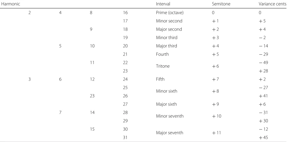
One challenge of MPE is overlapping partials [9,10] (the spectra of different notes share many common frequency bins with each other). It is an inevitable result caused by temperament relationships and vibration properties. For example, Table 1 gives the frequency relationship between the first 30 overtones of a reference note and its upper octave under exact equal temperament assumption.
*Correspondence:[email protected]
1Department of Mathematics, Jilin University, Changchun, China Full list of author information is available at the end of the article
Given a reference notenand its fundamental frequency f, denoting semitone shifts as subscripts, the fundamen-tal frequency ofn’s fifth note (seven semitones aboven), for instance, isf7=f ×2
7
12. According to the equal tem-perament, the interval from f7’s first octave tof’s third overtone is about 2 cents (1200∗log2
3f
2f7
≈ 2, refer to the 9th row of Table1). Analogically, we have the interval fromf3’s fourth octave to f’s 19th overtone is about −2 cents (1200∗log22194ff
3
≈ −2, refer to the 4th row of Table1). One can easily testify the rest of the table.
Besides, the acoustical characteristics of different instruments make the problem even more difficult: on the one hand, timbre variation results in different overtone magnitude distributions; on the other hand, inharmonicity2 leads to various overtone frequency dis-tributions [11]. Pianos are especially harder to deal with than other stringed instruments due to the complicated way of strings being wired. Due to the inharmonicity and its uniqueness on different strings [11], the slight fre-quency mismatch between the first overtone of a note and its upper octave will cause an interference pattern (a.k.a. acoustic beat) if pianos are tuned by exact equal tempera-ment. In order to eliminate such acoustic beats, pianos are usually tuned individually by well-trained experts (called
Table 1Frequency relationships between the overtones of a reference notenand its upper octave
Harmonic Interval Semitone Variance cents
1 2 4 8 16 Prime (octave) 0 0
17 Minor second +1 +5
9 18 Major second +2 +4
19 Minor third +3 −2
5 10 20 Major third +4 −14
21 Fourth +5 −29
11 22
Tritone +6 −49
23 +28
3 6 12 24 Fifth +7 +2
25
Minor sixth +8 −27
23 26 +41
27 Major sixth +9 +6
7 14 28
Minor seventh +10 −31
29 +30
15 30
Major seventh +11 −12
31 +45
Numbers under “Harmonic” indicate the overtone indices ofn. Column indices of “Harmonic” indicate the octave numbers starting from 0. Variance cents in the last column are rounded up into integers
harmonic tuning, the deviation from the exact equal tem-perament often forms a Railsback curve [12]).
The other challenge of MPE comes from the complex-ity of note combination. Strategies for solving multi-label classification can be generally categorized into two, “one vs. all” and “one vs. one,” respectively. Let the class number ben, the former needsnclassifiers while the latter needs
n 2
= n2−n
2 ones. Although it is computationally fea-sible for most circumstances, classifiers are trained inde-pendently from feature extraction. The lack of supervision in feature extraction may degrade the performance since it is more meaningful for features to minimize classifica-tion error rather than reconstrucclassifica-tion error [13]. Another existing strategy needs 2n classifiers by encoding multi-labels into single-multi-labels. It is only feasible when nis not large; otherwise, one may suffer from dimension explosion problem. Taking the piano for example, choosing 7 notes
from 88 yields
88 7
≈ 6.3×10⁹combinations. Even if only timbre and decay are included, it is almost impossible to construct and train such a large-scale dataset.
Moreover, as one of the most commonly used features in acoustic music processing applications, time-frequency representation is constrained by the uncertainty princi-ple. The algorithm performance then may be degraded by such deficient feature. Meanwhile, recent results have shown that feature fusion from different sensors (namely modality, one may consider someone’s fingerprint and iris, or footages of some action from different angles)
has advantages for recognition tasks (cf. [14–16] and references therein). Combined information from multi-ple sources is more robust and tolerant to noises and errors. Multimodal joint representation under constraints maximizes the utility of different features, which can be used more effectively in task-driven scenarios. Note that multimodal features are different from stacking multiple features into one because the latter does not take the modality relationship into account, and increasing dimen-sionality brings huge computation and storage costs.
Fig. 1Training structure of MPENet. Following Caffe terminology, this figure shows the computation graph of training phase. Arrows indicate blobs; rectangles and ellipses indicate Caffe built-in computation and loss layers. Hexagons indicate layer collections. Rounded rectangles indicate our implemented layers. All built-in layer names conform to Caffe. More details are explained in Sections3and4. Repeated elements of each modality are omitted by dashed lines
• Lorentzian-BlockFrobenius sparsity: A novel
· L−BF,γis imposed to a multimodal NMF model.
Penalty is determined by the magnitude of class templates of all modalities so that class sparsity can be ensured.
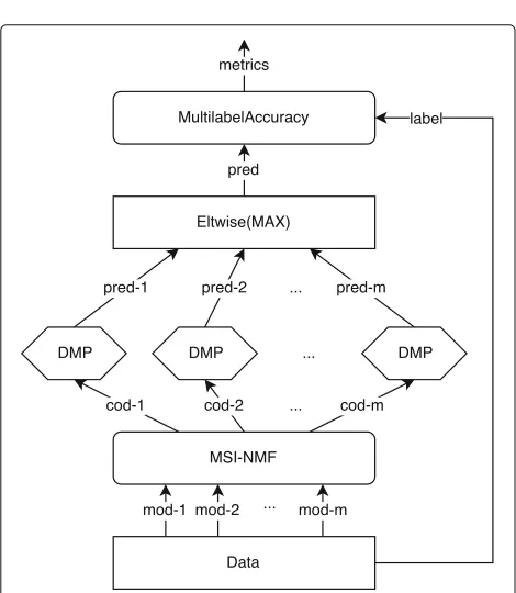
Fig. 2Test structure of MPENet. Following Caffe terminology, this
figure shows the computation graph of test phase. Legends can be referred to Fig.1. More details are explained in Sections3and4
• Multimodal sparse incoherent NMF layer: A new
deep learning layer based on the above constrained NMF model is presented. Sparse representations, as layer outputs, are computed by Alternating Direction Method of Multipliers (ADMM). Dictionaries, as layer parameters, are updated by Projected Stochastic Gradient Descent (PSGD). Incoherentness is added to the net loss as weight decay. Layer formulation and algorithms are given in Section3.
• Multipitch estimation network (MPENet) : Given the
decomposition capability of proposed layer, we employ “one vs. all” strategy and present a unified deep learning network consisting of a training subnet and a test subnet. Experiments show that the test net achieves state-of-the-art results by using only two modalities of monophonic samples as training data. Network details are explained in Section4.
2 Related work
samples of each note, (2) constructing a dictionary by concatenating all note templates, and (3) estimating mul-tiple notes by computing the codings with the dictionary fixed. In early studies, each template has only one atom (columns of a dictionary are called atoms). Weninger et al. [24] develop this simple structure by dividing note sam-ples into two parts: onset and decay. Then, two atoms are learned respectively from both parts, which yields a two-column note template. Such dictionary helps to cap-ture the feacap-ture variation and distinguish note state over time. O’Hanlon and Plumbley [25] take a further step on dictionary flexibility. Note templates are constructed by using linear combinations of several pre-defined fixed narrow-band harmonic atoms. The input spectral data is then approximated underβ-divergence group sparsity constraint. Other methods employing similar idea but different implementations are proposed in [2,4, 26–29]. Such procedure uses fixed dictionary to get note activa-tions during test, so MPE results heavily depend on the learned note templates, i.e., training samples. One has to retrain each template once new samples are added into training set. For other work using NMF with row/group sparsity and incoherent dictionaries, refer to [30–32] and references therein. Note that there are also studies that use unsupervised NMF instead of training note templates via isolated note samples. Bertin et al. [33] propose a temper-ing scheme favortemper-ing NMF with Itakura-Saito divergence to global minima. O’Hanlon and Sandler [34] propose an iterative hard thresholding approach for l0 sparse NMF problem with Hellinger distance. ERBT spectrograms of polyphonic music pieces are decomposed directly and a pitch salience matrix is calculate to detect active notes. A semi-supervised NMF method can be referred to [35].
Many non-NMF based algorithms have been proposed for MPE problem. Tolonen and Karjalainen [36] divide the signal into two channels according to a fixed frequency and compute autocorrelation of the low channel and the envelope of the high channel to form summary autocorre-lation function (SACF) and enhanced SACF (ESACF). The SACF and ESACF representations are used to observe the periodicities of the signal and estimate notes. Klapuri [37] calculates the salience representation through a weighted summation of overtone amplitudes. Three estimators based on direct, iterative, and joint strategies are pro-posed to extract notes from the salience function. Emiya et al. [1] employ a probabilistic spectral smoothness prin-ciple to iteratively estimate polyphonic content from a set of note candidates. An assumption of maximum num-ber of concurrent notes (nmax = 6) is imposed to avoid extracting overmany notes. Adalbjörnsson et al. [3] use a fixed dictionary to reconstruct input signal under block sparsity constraint. Notes are then identified through coding magnitudes. The fixed dictionary used here, how-ever, is constructed according to equal-tempered scale
so that the algorithm is unsuitable for instruments with inharmonicity.
Deep learning has been used to address AMT prob-lem in recent papers. Sigtia et al. [38] presents a real-time model which introduces recurrent neural networks (RNN) into a convolutional neural network (CNN, with only convolution, pooling, and fully connected layers). Kelz et al. [39] compare the performances of networks with different types of inputs (spectrograms with lin-early/logarithmically spaced bins, logarithmically scaled magnitude, and constant-Q transform), layers (dropout and batch normalization), and depths. Hawthorne et al. [40] propose a deep model with bidirectional long short term memory (BiLSTM) networks and two objective func-tions (onsets and frames), achieving state-of-the-art per-formance on MAPS [1] under configuration 2 described in [38]. For more acoustic music processing work using deep learning, refer to [40] and references therein. Note that the deep learning methods listed here all use music pieces as training data, which means polyphonic information can be accessed, hence music language model and classifiers are learned simultaneously.
3 Multimodal sparse incoherent NMF layer
3.1 Notation
Throughout this paper, we denote vectors and matrices by bold lowercase and uppercase letters, for example,v∈Rm
andM∈Rm×n. Parts of vectors and matrices are denoted by subscripts:viis the i-th entry ofv;Mi,Mi→,Mi,j, and
Mi,j,p,qrepresent the i-th column, i-th row, (i, j)-th entry, andp×qblock starting from (i, j)-th entry, respectively. ·,·denotes the inner product of two vectors. Forp1, thelpnorm ofvis defined asvp mi=1|vi|p
1
p, and
the Frobenius norm ofMasMF
i,jM2i,j
1 2
. Projec-tion operator and indicator funcProjec-tion of a setCwith respect to a pointxare respectively defined as
C(x)argmin y∈C y−x
2
2, δC(x)
0, x∈C
∞, otherwise
For notation simplicity, we also defineNm{1, 2,. . .,m},
R0{x|x∈R,x0}.
3.2 Prototype
Mlp,1 d
i=1
Mi→p, M∈Rd×m, p1 (1)
It enforces dictionaries of different modalities using same atom to present same event, for example,l2,1encourages collaboration among all modalities, andl1,1imposes extra sparsity within rows.
For MPE problem, dictionary incoherentness should be imposed to provide flexibility of modeling universal note representations in contrast to redundancy. As we dis-cussed in Section1, single-atom note templates cannot cover the diversity of music spectra whereas NMF can-not guarantee the stability and uniqueness for multi-atom ones. Because harmonic tuning aggravates overlapping partials, we can not distinguish that a spectral peak is a note overtone or a summation of several ones, i.e., it is not feasible to decompose frequency domain into orthog-onal bins according to the center frequencies of harmonic series. In order to detect notes directly from factorization, a “good” dictionary should be trained under the supervi-sion of data and task, possessing the following properties: (1) note templates are mutually discriminative and (2) for a certain note, all possible variants can be and only can be represented by its templates.
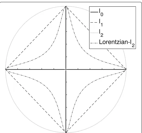
Moreover, we improvelp,1 norm for two reasons. The first one is coding structure does not satisfy row-wise sparsity since dictionary incoherentness is imposed. Note samples are approximated by linear combination of its template atoms. The second one isl1norm imposes too much penalty so that every activation is either scaled down or zeroed out by soft threshold shrinkage [44]. For unknown number and loudness in MPE problem, each coding entry is crucial for detecting notes correctly, so we want to preserve as many effective activations as possible. Opposed to l1 and l2, the Lorentzian-l2 norm [45]3, defined as
vL−l2,γ d
i=1 log
1+ v 2
i
γ2
, v∈Rd, γ 0 (2)
penalizes large activations with small weights but the other way around so that non-zero activations keep their contributions. Besides,l1norm is not differentiable at 0, which makes the computation of gradient complicated ([15] tackles this by introducing “active set”). The every-where smoothness of Lorentzian-l2 provides good con-vergence property. Figure3shows the contours of several common regularizations.
Summing up the above discussion, the prototype of multimodal sparse incoherent NMF layeris a multimodal sparse incoherent NMF model whose cost function is, given multimodal inputxi∈Rf
i
0,i=Nm
,
Fig. 3Contours of several norm regularizations are discussed here
lDi,A;xi
min A∈A,Di∈Di
m
i=1 ⎛ ⎝1
2D iA
i−xi22+μ 2
d
j=1
d
k=1,k=j
Dij,Dik
2 ⎞ ⎠
(3)
+λ1AL−BF,γ+ λ2 2 A
2
F, μ >0,λ1>0,λ2>0
where superscripts indicate modality indices,mdenotes modality number, f denotes feature dimensionality, n denotes class number, a denotes atom number of each class template, d = n× a is dictionary column num-ber, and{μ,λ1,λ2} are penalties.A
M|M∈Rd×0m
is coding space;Di N|N∈Rfi×d
0 ,Nj21,j=Nd
are dictionary spaces. Lorentzian-BlockFrobenius norm is defined as
AL−BF,γ n
i=1 log
1+Ai 2
F
γ2
,AiA(i−1)a+1,1,a,m,γ >0
In (3), Ai contains all template coefficients of the
([42, 44, 46, 47]) split (3) into two subproblems, sparse coding and dictionary learning, respectively.
3.3 Structure
MSI-NMF layer is constructed by re-translating the two subproblems of (3), where we treatAas layer outputs and
Di,i=Nmas layer parameters. Using the same network notations as in Section 1, Fig. 4 shows the structure of MSI-NMF layer, where layer parameters are denoted by texts within parentheses.
3.4 Forward pass
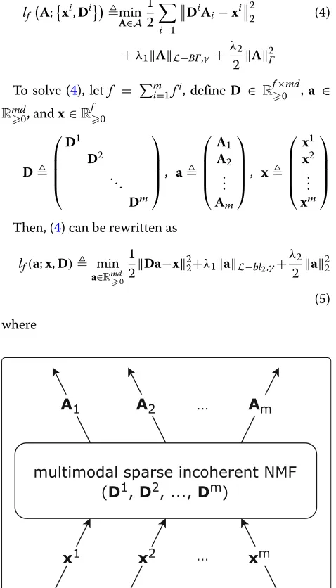
The forward pass produces the solution of a multimodal non-negative sparse coding problem whose cost function is defined as
lf
A;xi,Dimin
A∈A 1 2
m
i=1
DiAi−xi22 (4)
+λ1AL−BF,γ+λ2 2 A
2
F
To solve (4), letf = mi=1fi, defineD ∈ Rf×0md, a ∈
Rmd
0, andx∈R
f 0 D ⎛ ⎜ ⎜ ⎜ ⎝ D1 D2 . .. Dm ⎞ ⎟ ⎟ ⎟ ⎠, a
⎛ ⎜ ⎜ ⎜ ⎝ A1 A2 .. . Am ⎞ ⎟ ⎟ ⎟ ⎠, x
⎛ ⎜ ⎜ ⎜ ⎝ x1 x2 .. . xm ⎞ ⎟ ⎟ ⎟ ⎠
Then, (4) can be rewritten as
lf(a;x,D) min a∈Rmd
0 1
2Da−x 2
2+λ1aL−bl2,γ+
λ2 2 a
2 2
(5)
where
Fig. 4Structure of MSI-NMF layer. Legends can be referred to Fig.1.
Following Caffe terminology, arrows indicate tensors (Caffe blobs), and dictionaries (Di,i=Nm) are treated as layer parameters
aL−bl2,γ n
i=1 log
1+ a˜i
γ2
(6)
˜
ai= m
j=1
a
k=1
a2(j−1)d+(i−1)a+k (7) (5) can be solved usingAlternating Direction Method of Multipliers(ADMM, ref. [44,46,47]), details are given in Algorithm 1 (proofs in Appendix), where is given in Algorithm 2.
Algorithm 1Forward Pass of Multimodal Sparse Incoher-ent NMF Layer: Multimodal Non-negative Sparse Coding
Require: D,x,a(0) = 0md,b(0) = 0md,λ1 > 0,λ2 > 0, γ >0,ρ >0 andk=1
1: repeat
t=DTD+(ρ+λ2)I −1
DTx+ρa(k−1)−b(k−1) u=Rmd
0
b(k−1)+t
a(k)= (u,λ1,ρ,γ ), using Algorithm 2
b(k)=b(k−1)+t−a(k)
k=k+1
2: until aconverges
Ensure: a
3.5 Backward pass
The backward pass is to update D through gradient descent. The incoherentness constraint is treated as weight decay of layer parameters. Denoting the network cost function bylnet, the new cost function becomes
lnewlnet+μ 2
m
i=1 ⎛ ⎝d
j=1
d
k=1,k=j
Dij,Dik
2 ⎞
⎠ (8)
Then, we have
∂lnew ∂Dp,q =
∂lnet ∂Dp,q +
μ
2
∂m
i=1
d j=1
d k=1,k=j
Dij,Dik2
∂Dp,q
(9)
wherep= Nf,q= Nmd. According to the chain rule, the first term of (9) is
∂lnet ∂Dp,q =
∂
lnet ∂a ,
∂a
∂Dp,q
(10)
In order to get ∂D∂a
p,q, recalling thatais a minimizer of
(5), taking the derivative w.r.ta, we have
Algorithm 2 : Inner Update Algorithm of a in Algorithm 1
Require: u,λ1,ρ,γ,λ = λ1ρ,σ = 2λ+γ2,p = 0nand
a=0md
1: forj=1, 2,. . .,ndo
u= m
l=1
a
k=1
u2(l−1)d+(j−1)a+k (12)
2: ifu=0then
pj=0
3: else
4: ifλ4γ2then
5: ifγ2= 271 andλ=4γ2then pj=
1 3
6: else
A=u2−3uσ, B=9uγ2−uσ,C=σ2−3uγ2,=B2−4AC
y1,2= 3
u 2
2A+3B±√
pj= 1 3+
y1+y2 3u
7: end if
8: else
9: if >0thengoto6
10: else if=0then
K= B
A, y1=1+K, y2= − K
2
pj= argmin x∈{y1,y2}∩[0,1]
λlog
1+ u
γ2x 2
+u
2(x−1) 2
11: else
θ = arccos
u2 A√A
2u−9σ+9γ2
3
y1= 1 3−
√
A(cosθ+sinθ)
3u , y2=
1 3+
2√Acosθ 3u
pj= argmin x∈{y1,y2}∩[0,1]
λlog
1+ u
γ2x 2
+u
2(x−1) 2
12: end if
13: end if
14: end if 15: end for
16: forj=1, 2,. . .,mddo
aj=ujpk, k= j/amodn
17: end for
Ensure: a ˜ W= ⎛ ⎜ ⎜ ⎜ ⎝ W W . .. W ⎞ ⎟ ⎟ ⎟ ⎠ (13) W= ⎛ ⎜ ⎜ ⎜ ⎝
w1I
w2I . ..
wnI
⎞ ⎟ ⎟ ⎟
⎠ (14)
wi= 2
γ2+ ˜ai, i=N
n (15)
˜
ais defined in (7). Then, ∂lnew
∂Dp,q can be computed because
∂a
∂Dp,q can be obtained by taking the derivative w.r.tDp,qon
(11) and ∂lnet
∂a is given by the last layer.
The backward algorithm of proposed layer is listed in Algorithm 3 (proofs in Appendix), whereVi ∈ Rd×n is defined as Vi ⎛ ⎜ ⎜ ⎜ ⎝
A1,i,a,1
Aa+1,i,a,1 . ..
A(n−1)a+1,i,a,1 ⎞ ⎟ ⎟ ⎟
⎠ (16)
i = Nm, diag(M)is a diagonal matrix whose diagonal entries come fromM, andUi∈Rd×d.
Algorithm 3Backward Pass of Multimodal Sparse Inco-herent NMF Layer: Multimodal Non-negative IncoInco-herent Dictionary Learning
Require: Di,xi,i=Nm,A, ∂lnet
∂A,λ1>0,λ2>0,γ >0,
μ >0 andη1>0 1: computeW˜ using Eq.(13)
2: for i=1, 2,. . .,mdo
3: generateViusing the definition in Eq.(16) 4:
Ui=DiTDi−diagDiTDi (17)
5:
Pi=DiTDi+λ1W
I−WViViT+λ2I (18) 6:
Qi=Pi−T∂lnet Ai
(19)
7:
∂lnew ∂Di =
xi−DiAi
QiT−DiQiATi +μDiUi (20)
8:
Di←Di
Di−η1∂
lnew ∂Di
(21)
9: end for
4 MPENet
In this section, we detailedly explain the layer and tensor specifics of MPENet. In order to avoid misunderstand-ings caused by layer names in different deep learning frameworks (for example, commonly called “fully con-nected” is named as “inner product” in Caffe, “linear” in PyTorch, and “dense” in TensorFlow), during illustration, we will give the mathematics expression of some layers if necessary. Meanwhile, in order to give the most direct ideas of how MPENet is constructed, we switch to Caffe terminology accordingly (see Figs.1and 2).
In Figs. 1 and 2, training and test phases have same core modules, differences only locate in the top lay-ers. “Data” layer produces multimodal features and their labels. Labels are binary vectors whose entries are 1 if corresponding classes are active and 0 otherwise. “Sig-moidCrossEntropyLoss” layer is a stack of “sigmoid” layer and “cross-entropy” layer. Cross-entropy loss is defined as
−1
n n
i=1
pilogpˆi+(1−pi)log1− ˆpi, p,pˆ ∈Rn
wherepandpˆare predictions and labels. 4.1 Deep multi-label prediction module (DMP)
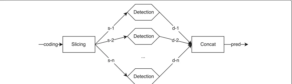
The structure of “Deep Multi-label Prediction” (DMP) is shown in Fig. 5. “Slicing” layer segments an n × a vector into n parts. “Detection” is a classifier module with replaceable structure, and is supposed to output the existence magnitude according to the input. “Concat” (concatenation) layer jointsndetections to form a multi-label prediction. In our experiment, five layers are used to implement “Detection” module (structure is shown in Fig.6). “InnerProduct” represents the transform fromx∈
Rmtoy∈Rn
y=Wx+b, W∈Rn×m,b∈Rn
“ReLU” (Rectified Linear Unit) stands for the transform fromx∈Rmtoy∈Rm
yi=max(xi, 0), i=Nm
For other tasks, one can modify this combination accordingly.
The reason for such structure roots from the property of incoherent dictionaries. If samples of certain class can be and only can be represented by its template atoms, the existence of this class is only related to the coeffi-cient magnitudes. “One vs. all” strategy can be employed natively. If dictionaries are not as good as expected, cross-entropy loss will correct each “detection” module as well as dictionaries of the proposed layer through backward pass, which completes a positive circle.
4.2 Multi-label accuracy layer
Multi-label accuracy layer is implemented to conduct training and test in a unified framework. It consists of three sequential operations: sigmoid activation, binary output, and metric computation. The second one out-puts either 0 or 1 according to the comparison result between the sigmoid activation and a predefined thresh-oldt. The third one calculates the Precision (P), Recall (R), and F-measure (F) according to the binary outputs and the ground truths, where
P= TP
TP+FP, R= TP
TP+FN, F=
2×P×R P+R
TP,FP, andFNstand for true positive, false positive, and false negative, respectively.
5 Experiment results
In this section, we first briefly demonstrate the dataset and features used in our experiment, then illustrate parameter initialization and network configuration in detail. Piano MPE results, experiment results about how MPENet
Fig. 6Structure of “Detection” implemented in our experiment. Legends can be referred to Fig.1. All built-in layer names conform to Caffe. Details can be referred to Section4.1
works, timbre robustness results, and AMT results are given in the end of this section.
5.1 Dataset and features
MAPS [1] is a commonly used piano dataset for multipitch estimation and automatic transcription. It contains nine kinds of recording conditions (referred to as “StbgTGd2,” “AkPnBsdf,” “AkPnBcht,” “AkPnCGdD,” “AkPnStgb,” “Sptk-BGAm,” “SptkBGCl,” “ENSTDkAm,” and “ENSTDkCl”), two of them (“ENSTDkAm” and “ENSTDkCl”) are from real pianos and seven are synthesized by softwares. Each kind has same subset hierarchies which include ISOL (monophonic recordings), RAND (random combination), and UCHO (chords).
ISOL/NO subset, which contains 264 monophonic wav files covering 88 notes (n = 88) and 3 loudness levels, is used as training set. RAND subset, which contains 6 polyphony levels ranging from 2 to 7 (labeled as P2–P7), is used as test set. Each one of P2–P7 has 50 files, and the note combination of each file is generated randomly. In [1], a 93-ms frame which is 10 ms after onset of each file in P2–P6 is analyzed. As comparison, we conduct similar evaluation in our experiment. P7 is used as validation set for parameter tuning.
Each wav file in MAPS is stereo with sampling rate 44100 Hz. To extract features, we firstly generate a mono counterpart by averaging both channels. Then, the silent part of each counterpart is truncated according to the provided onsets and offsets. Finally, two kinds of fea-tures (m = 2) are extracted from the remainder by Short Time Fourier Transform (STFT) and Constant-Q Transform (CQT). The reason for using STFT and CQT is mainly because the former has good resolution in high-frequency domain while the latter does well in low-frequency domain. STFT and CQT features are further transformed into non-negative dB scale using
h(·) log10(·/+1)
log10(1/+1) (22)
where · is either CQT or STFT feature and is the machine precision. Other extraction specifics are listed in Table 2, where flen, slen, minf, maxf, dim, ppo, and nfft are abbreviations for frame length, step length, min-imal frequency, maxmin-imal frequency, dimensionality, par-tition per octave, and n-point Fast Fourier Transform, respectively.
5.2 Parameter initialization
Due to the non-convexity of problem (3), only local min-imization can be guaranteed. The initial value of dictio-naries is crucial for convergence and performance. Since totally random initialization makes the codings of first several epochs meaningless, it is a waste of time and computation resources. Plus, because each monophonic file in the training set lasts for over 2 s, many samples are similar to each other during decay. It is not reason-able to initialize the dictionary using random samples as most dictionary learning algorithms do [15] either. In our experiment, two procedures are employed to initialize the dictionary.
To avoid the heavy overhead caused by joint learn-ing of dictionaries and classifiers, before really get-ting into MPENet, we propose a pre-learning phase called Label Consistent Incoherent Dictionary Learning (LCIDL) derived from [48, 49] to obtain a better start than random initialization and sample initialization for dictionaries in MSI-NMF layer. The cost function of LCIDL is
llc
Di,A;xi
min A∈A,Di∈Di
m
i=1 ⎛ ⎝1
2D iA
i−xi
2 2+
μ
2 d
j=1
d
k=1,k=j
Dij,Dik
2 ⎞ ⎠
(23)
+λ1AL−BF,γ+ λ2
2 L−A 2
F
whereL∈Rd×m(referred to asdiscriminative coding) is, ifxi,i=Nmbelongs to the j-th note,
L=
⎛ ⎜ ⎝
L1 .. .
Ln
⎞ ⎟
⎠, Lk= 1
a×m, k=j
0a×m, otherwise , k=R n
It is worth emphasizing that (23) is a plain data-driven problem, and neither MPENet nor classifiers are involved
Table 2Feature specifics used in MPENet
Flen (ms) Slen (ms) Minf (Hz) Maxf (Hz) Dim Misc
CQT
23.2 6.5 27.5 7000 576 ppo:72
0 0.1 0.2 0.3 0.4 0.5 0.6 0.7 0.8 0.9 1 Recall
0 0.1 0.2 0.3 0.4 0.5 0.6 0.7 0.8 0.9 1
Precision
X: 0.7092 Y: 0.9137
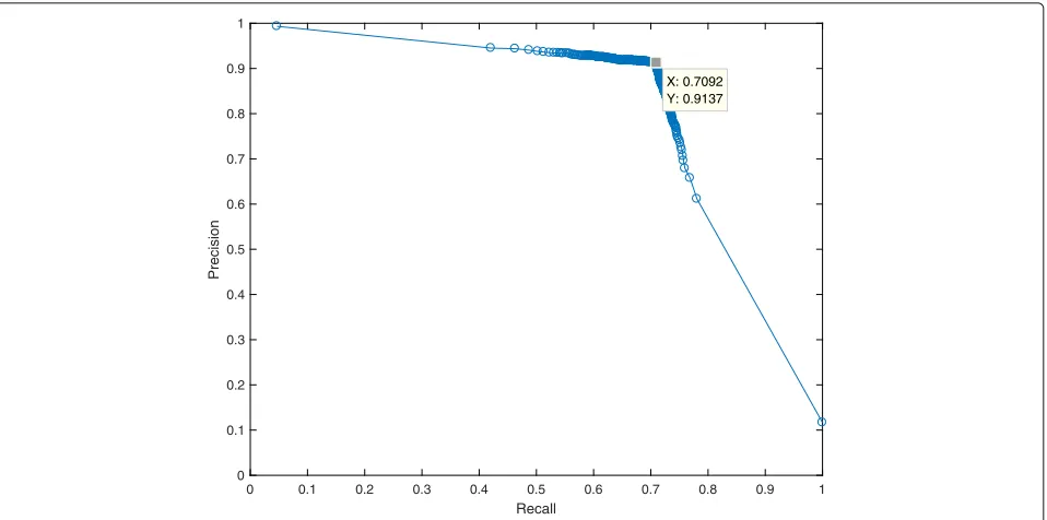
Fig. 7Precision-Recall Curve of P7. “Detection” module produces similar results whentvaries in a relatively large interval around 0.5, the best result
is shown by a gray square
at the time. It has nothing to do with deep learning and can be implemented by any language. The form ofLis the extension of binary labels to impose classification infor-mation, because there are no note probabilities but only codings on our hands.
Likewise, LCIDL also needs a good dictionary to start for acceleration. In order to find it and determine the atom number, a fast clustering algorithm based on density peaks [50] is employed to filtrate samples hierarchically. Specifi-cally speaking, we first extract 30 cluster centers from each modality of each file in the training set. Then, we stack them according to their note indices. This gives us two matrices with 810 columns for each note (810 = 30×3 (loudness) ×9 (recording)). Finally, through computing density peaks on these two matrices and considering the overhead and efficiency of computation and storage, we empirically set the atom number of each note template to
Table 3Precision (%) result with unknown polyphony level
P2 P3 P4 P5 P6
Tolonen [36] 47 46 51 53 48
Tolonen-500 [36] 58 59 59 60 50
Klapuri [37] 94 92 88 84 84
Emiya [1] 97 95 92 91 91
MPENet 95.29 93.26 92.76 92.21 90.52
be 15 (i.e.,a= 15 in (3)) and obtain a 576×1320 matrix and 648×1320 matrix for starting LCIDL.
After LCIDL is done, we obtain a “roughly good” dictio-nary, it has low reconstruction loss, incoherentness, and coding shape likeLas (23) governs. When the real train-ing of MPENet begins, this “roughly good” dictionary is copied into MSI-NMF layer, and classifiers are initialized randomly. During the first several epochs of training, the learning rate of classifiers is relatively larger than that of MSI-NMF since we want to hold codings a little bit to fit classifiers first. As the classification error decreases, the learning rates of all layers become equal to do joint learning.
5.3 Network configuration
Choices of parameters used in MPENet are all empiri-cal. The output numbers of three “InnerProduct” layers
Table 4Recall (%) result with unknown polyphony level
P2 P3 P4 P5 P6
Tolonen 58 43 35 30 28
Tolonen-500 77 68 52 45 32
Klapuri 89 88 83 78 62
Emiya 90 82 71 63 47
Table 5F-measure (%) result with unknown polyphony level
P2 P3 P4 P5 P6
Tolonen 53 45 42 38 33
Tolonen-500 65 63 57 51 40
Klapuri 91 90 86 81 72
Emiya 93 87 80 75 63
MPENet 97.11 94.25 90.08 86.89 83.65
in Fig.6are set to be 60, 30, and 1 from left to right. All three layers use bias term. For MSI-NMF layer, we use
λ1 = 0.15,λ2 = 0.1, μ = 1.32, ρ = 0.2, γ = 1.09, andt = 0.5 for training. Considering that only one note is active at a time during training whereas at least two are active concurrently during test, test constraints should be weaker than those of training. Limited by the computa-tion overhead, a fully greedy search cannot be done to get the best result. Therefore, we initialize several groups of parameters, and the one withλ1 = 0.03,λ2 = 0.1,μ = 1.32,ρ = 0.2, andγ = 0.55 gets the best result through evaluating the test net on P7. To tune binary threshold tof multi-label accuracy layer, we plot a Precision-Recall Curve in Fig.7according to the evaluation result on P7, where t ranges from 0 to 1 with step 0.001. Through the figure, we find that “detection” modules produce very polarized outputs. The best result (91.37% Precision and 70.92% Recall, see the gray square in Fig.7) and similar ones can be achieved whent is within a relatively large interval around 0.5. Therefore, we keept=0.5 unchanged for test.
5.4 MPE results
Evaluation metrics are listed in Tables3,4, and5when the polyphony level is unknown. Our network outperforms all other algorithms on Recall and F-measure. Precisions of P2, P3, and P6 get the second best results with slight gaps compared to Emiya’s. The decrease of sparsity constraint is the reason for this result shortage. During evaluation, we can achieve over 99.9% F-measure for P2 and P3 if we use training parameters. Such configuration can also maintain high Precision results for P4–P6; however, Recall will drop dramatically due to strong sparsity. It is a trade off and contradiction between sparsity and concurrent notes.
We also report the evaluation results in Table6when polyphony level is known as prior. For polyphony level k, we choose the indices of first k largest outputs
Table 6F-measure (%) result with known polyphony level
P2 P3 P4 P5 P6
99.78 94.48 86.91 85.13 80.42
in sigmoid layer as active notes. Results show that F-measure increases for P2 and P3 while things are dif-ferent for P4–P6. It states a fact that when concurrent number is small, the ground truths have higher probabil-ities than others in our algorithm; as concurrent number grows, undetected ground truths become undetectable.
5.5 How MPENet works
In order to show how each key part of MPENet con-tributes to the performance, we conduct four groups and seven in total experiments. Considering the combination complexity, each experiment only changes single part to show its impact on the system. Group indices, names, and settings are listed in Table7, where√and×indicate pres-ence and abspres-ence, respectively; the setting described in Sections5.3and5.4is calledMPENet-default (MPENet-d for short). Unless otherwise specifie(MPENet-d, all experiments in this subsection share same parameters with MPENet-d except the moMPENet-difieMPENet-d part. Implementation MPENet-details anMPENet-d results are explained in the following subsections.
5.5.1 Modality
Config.1 and Config.2 use single modal features listed in Table 7as training inputs to show our multimodal effi-cacy. Results are plotted in Fig. 8. We find that STFT’s Precision outperforms CQT’s on all test sets, while the STFT’s Recall decreases substantially from P3. MPENet-d, as expected, incorporates the advantages of both modali-ties and amend their drawbacks.
5.5.2 Atom number
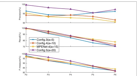
Group 2 (Config.3–Config.5), in conjunction with MPENet-d, shows the influence of atom number on our system. We only changeadescribed in Section5.2to ini-tialize dictionaries with different sizes. Results are plotted in Fig.9. Interestingly, the Precision of each one in group 2 gets improvement except P2 of Config.4. Especially, the
Table 7Experiment settings for part comparison, where group 1 corresponds to modality variation only, group 2 to atom number, group 3 to joint learning, and group 4 to dictionary
incoherentness
Group Name Modality (m) Atom number (a)
Incoherentness Joint learning
1 Config.1 CQT 15 √ √
Config.2 STFT 15 √ √
2 Config.3 CQT&STFT 5 √ √
Config.4 CQT&STFT 10 √ √
Config.5 CQT&STFT 20 √ √
3 Config.6 CQT&STFT 15 √ ×
4 Config.7 CQT&STFT 15 × √
85 90 95 100
Precision(%)
40 60 80 100
Recall(%)
P2 P3 P4 P5 P6
60 70 80 90 100
F-measure(%)
Config.1(CQT) Config.2(STFT)
MPENet-d(CQT&STFT)
Fig. 8Modality comparison results. Precision, Recall, and F-measure are shown in three subplots from top to bottom, respectively, whereyaxis
indicates percentage value andxaxis indicates polyphony level. Three subplots share same legends
90 95 100
Precision(%)
70 80 90 100
Recall(%)
P2 P3 P4 P5 P6
80 85 90 95 100
F-measure(%)
Config.3(a=5) Config.4(a=10) MPENet-d(a=15) Config.5(a=20)
Fig. 9Atom number comparison results. Precision, Recall, and F-measure are shown in three subplots from top to bottom, respectively, whereyaxis
90 92 94 96 98
Precision(%)
60 70 80 90 100
Recall(%)
P2 P3 P4 P5 P6
70 80 90 100
F-measure(%)
Config.6(without joint learning) MPENet-d(with joint learning)
Fig. 10Joint learning comparison results. Precision, Recall, and F-measure are shown in three subplots from top to bottom, respectively, wherey
axis indicates percentage value andxaxis indicates polyphony level. Three subplots share same legends
P2 P3 P4 P5 P6
0 0.1 0.2 0.3 0.4 0.5 0.6 0.7 0.8 0.9 1
AkPnStgb AkPnCGdD AkPnBsdf AkPnBcht ENSTDkAm StbgTGd2 SptkBGCl SptkBGAm
P2 P3 P4 P5 P6 0
0.1 0.2 0.3 0.4 0.5 0.6 0.7 0.8 0.9 1
AkPnStgb AkPnCGdD AkPnBsdf AkPnBcht ENSTDkAm StbgTGd2 SptkBGCl SptkBGAm
Fig. 12Recall results of timbre robustness experiment
P2 P3 P4 P5 P6
0 0.1 0.2 0.3 0.4 0.5 0.6 0.7 0.8 0.9 1
AkPnStgb AkPnCGdD AkPnBsdf AkPnBcht ENSTDkAm StbgTGd2 SptkBGCl SptkBGAm
Precision increase of Config.5 (a=20) for all test sets and that of Config.3 (a= 5) for P5–P6 are substantial. While the Recall for P2 are all close to each other, and Config.5’s Recall remains approximately equal to MPENet-d’s for P2–P5, Config.3’s Recall and Config.4’s (a=10) decrease a little. As a result, the F-measures of Config.3 for P2 and Config.5 for P2–P4 are slightly higher than that of MPENet-d. Such result implies that MPENet becomes robust to polyphony level under same parameters as atom number increases. We think the reason for oscillated metrics is parameters still have strong influences on the outputs in this situation. Although Config.5 performs better than MPENet-d for P2–P5, considering time complexity (∝ Opmn2√κDTD+(ρ+λ2)I
for conjugate
gradient method or∝ Opmn3for Cholesky decompo-sition method, where p is ADMM iteration number, κ is condition number,m,n,Dare defined in (5)) and the F-measure of P6, we consider MPENet-d sufficient enough. For those with unlimited computation resources, one can modify a and re-validate corresponding parameters for better performances.
5.5.3 Joint learning
Config.6 (without joint learning) is implemented by divid-ing dictionary and classifier learndivid-ing as separate opera-tions. During training, we first learn dictionaries by using
Table 8Frame-level AMT results using 60 full-length music pieces in “ENSTDkCl/MUS” and “ENSTDkAm/MUS”
Precision (%) Recall (%) F-measure (%)
Hawthorne [40] 88.53 70.89 78.30
Sigtia [38]* 71.99 73.32 72.22
Kelz [39]* 81.18 65.07 71.60
Melodyne [40] 71.85 50.39 58.57
MPENet 90.14 48.96 62.95
Final metrics are the average over all pieces Results with asterisks are reimplemented by [40]
(23) in Section 5.2 since it is the only way to impose supervision. Then, we compute the codings of mono-phonic training data by using (4) with learned dictionaries. Finally, monophonic codings are directly fed into “dmp” modules plotted in Fig.1to train classifiers. During test, we first compute the codings of polyphonic test data in P2–P6, then use the test phase in Fig.2 to get metrics. Note that dictionaries are only learned once and do not change any more during coding computation and clas-sifier training. Comparison results are shown in Fig.10, where we find that although Config.6 beats MPENet-d by 2% constantly on Precision, the Recall of Config.6 has increasing gap compared with MPENet-d’s as polyphony
0 7 15 22 29
time(s) 10
20 30 40 50 60 70 80
note index
Fig. 14AMT results of the first 30 s of “MAPS_MUS-bk_xmas5_ENSTDkCl” produced by plain MPENet, where green indicates true positives, red
0 7 15 22 29 time(s)
10 20 30 40 50 60 70 80
note index
Fig. 15AMT results of the first 30 s of “MAPS_MUS-deb_clai_ENSTDkCl” produced by plain MPENet, where legends can be referred to Fig.14. A
typical case of false negatives is where notes have long duration (still, MPENet can detect the attack of each note, but decays are discontinuous since the note probabilities are polarized caused by non-linear classifiers, c.f Fig.7)
level grows. As a result, MPENet-d outperforms Config.6 greatly on F-measure for P4–P6.
5.5.4 Dictionary incoherentness
For Config.7 (without dictionary incoherentness), we remove the incoherentness regularization in (3). Due to the absence of incoherentness, block sparsity makes no sense then. The cost function used in Config.7 becomes
lDi,A;xi (24)
min A∈A,Di∈Di
m
i=1
1 2D
iA i−xi22
+λ1AL−rl2,γ+
λ2 2 A
2
F
where Lorentzian-Row_l2is defined as
AL−rl2,γ d
i=1 log
1+Ai→ 2 2 γ2
The corresponding form of (23) then becomes
llc
Di,A;xi min A∈A,Di∈Di
m
i=1
1 2D
iA i−xi22
+λ1AL−rl2,γ +
λ2
2L−A 2
F
(25)
Forward and backward algorithm for (24) can be derived according to Algorithms 1 and 3. During training, we find the loss of training phase stays to a relatively high value (about two order higher than that of MPENet-d). Things do not change even if we reinitialize the parameters or train for extra several epochs. Moreover, during test, the sigmoid outputs of multi-label accuracy layer for P2–P6 are all less than the detection thresholdt, so the metrics of Config.7 are all zero, test fails.
Summing up the results, we find that incoherentness regularization is crucial for MPENet while modality, atom number and joint learning only affect performance. If sorting them by importance, we have
incoherentnessmodalityjoint learningatom number
5.6 Timbre robustness
label
Data
InnerProduct
InnerProduct
GRU
GRU
GRU
GRU
Concat
InnerProduct
ReLU
InnerProduct
SigmoidCross
EntropyLoss
Fig. 16Structure of the recurrent network used in AMT experiments.
The inputs are 16 time steps before and after current label. The number of hidden state of GRUs is 200, the output numbers of InnerProducts are all 200 except the last one is 88. Before concatenation, we only keep the last step’s output of each GRU because they accumulate all the information through time. Legends can be referred to Fig.1
noise and all other factors that can influence spectra may be very different from the other eight. The results in Figs. 11, 12, and 13 show that MPENet becomes over-fitting since all metrics of test sets drop fairly except “ENSTDkAm” (only recording condition is different from training set).
5.7 AMT results
Due to the underlying strong relationship between MPE and AMT, and in order to further explore the capacity of MPENet, we also conduct AMT experiments following configuration 2 described in [38]. Specifically speaking, we use total 60 full-length music pieces contained in the “MUS” subsets of “ENSTDkCl” and “ENSTDkAm” as input and run MPENet frame by frame. Parameters and hyper-parameters are all kept the same as “MPENet-d” (c.f Sections5.3and5.4). In line with the training phase of MPENet, the ground truths of music pieces are gen-erated by discretizing note durations provided in corre-sponding txt files. Table 8 gives the frame-level average
AMT results of MPENet, with comparison to state-of-the-art performance reported in [40]. MPENet maintains the Precision as in Section 5.4, but performs poorly on Recall. Figures 14 and15 reveal some occasions where false positives and false negatives take place, in which green indicates true positives, red indicates false negatives and blue indicates false positives. In brief, false positives consist of a few wrong chord detections and many scat-tered unrelated notes; while false negatives come from massive so-called super-combinations (number of simul-taneously active notes is over 7) and plenty of notes with long duration. The former circumstance of false nega-tives, as discussed in Section 5.4, is an inevitable result caused by sparsity constraints. For the latter circumstance of false negatives, however, we think the reasons behind such behaviors are mainly caused by two aspects: (1) the training set of MPENet lacks negative samples. Since training loss is not zero and recall the decay proper-ties of piano notes, classification errors of monophonic samples in training set include wrong detections and missing detections. The lack of negative samples makes MPENet tend to distinguish the beginning from the end of same note, which leads to insufficient durations; (2) MPENet knows nothing about music language, which prevents MPENet from rejecting scattered, unreasonable detections.
0 7 15 22 29 time(s)
10 20 30 40 50 60 70 80
note index
Fig. 17AMT results of the first 30 s of “MAPS_MUS-deb_clai_ENSTDkCl” after the regularization of recurrent network. Some false positives are
smoothed out. Note that since Gibbs sampling indices are selected randomly, not all frames have been updated by the recurrent network
have been updated during one full step. Also note that our recurrent network has way shorter memory than those in [38, 40], so it learns little music language and only has effects on scatted detections. Because AMT is not the concern of this paper, we do not experiment more here but maybe focus on possible AMT-related refinements in the future work.
6 Conclusions
In this paper, we propose a new deep learning layer based on a NMF model with multimodal inputs under sparsity and incoherentness constraints. Such “layeriza-tion” of optimization problem provides the possibility to learn dictionaries and other features jointly under a uni-fied deep learning framework. It enables modularization,
online learning, and parameter fine-tuning for dictionary learning problem, which can be used to simplify the model refactoring and extension. In comparison with the “high level” features produced by other deep learning layers, the proposed layer learns discriminative and represen-tative dictionaries so that the outputs are more realis-tically meaningful. Experiment results demonstrate that our test net improves the MPE performance substantially on MAPS dataset.
Restricted by hardwares, we pay more attention to layer algorithm and the network structure than model training. Unlike those fully explored and well-tuned deep learning models, MPENet with empirical parameters, simple layer combinations and shallow structures have plenty room for improvements. For future work, there are several direc-tions that can be considered: (1) from the layer point of view, performance grows with the increasing modality number. According to our experiment results, automatic parameter adaptation will also improve the estimation greatly; (2) from the network point of view, regularization, depth, and structure are new focuses for extracting more representative and robust features.
Endnotes
1Scientific Pitch Notation is used to represent notes, i.e.,
sub-contra octave is indexed by 0.
2For certain stringed instruments, overtones are close
to but not exactly integer multiples of the fundamental frequency, the degree of departure from whole multiples is called inharmonicity.
3Note that Lorentzian-l
2norm is not truly a norm since it satisfies all norm axioms except absolute homogene-ity, but we follow the convention of l0 norm and [45] throughout this paper.
Appendix
Proposition 1 aobtained by Algorithm1is a minimizer of (5).
ProofAlgorithm 1 is a straightforward application of ADMM. Introducingt,band using the notation in3.4, the unconstrained form of (5) is
1 2Dt−x
2
2+λ1aL−bl2,γ+
λ2 2 t
2 2+
ρ
2t−a+b 2 2+δRmd
0(a) (26)
Applying ADMM, the update scheme of (26) is
t=min t
1
2Dt−x22+ λ22t22+ ρ2t−a+b22 (27) ⎧
⎪ ⎪ ⎪ ⎪ ⎨ ⎪ ⎪ ⎪ ⎪ ⎩
a=min
a λ1aL−bl2,γ + ρ
2t−a+b22+δRmd
0(a) (28)
b=b+t−a (29)
Solving (27) yields
t=DTD+(ρ+λ2)I −1
DTx+ρ(a−b)
which is the update oftin Algorithm 1. To solve (28), we first change its form into
a=min a
λ1
ρ aL−bl2,γ+ 1
2t−a+b 2 2+δRmd
0(a) (30)
Denotingλ = λ1ρ and using Karush-Kuhn-Tucker con-ditions, we introducev∈Rmd0. The Lagrange function of (30) is
L(a,v)λaL−bl2,γ + 1
2t−a+b 2
2− v,a (31)
and KKT conditions are
(λW˜ +I)a=t+b+v (32)
ai0 (33)
⎧ ⎪ ⎪ ⎪ ⎪ ⎨ ⎪ ⎪ ⎪ ⎪
⎩vvi0 (34)
iai=0 (35)
wherei=NmdandW˜ is defined in (13). It is easy to find (32) can be split intonindependent groups
(λW+I)ai=ti+bi+vi, i=Nn (36)
where
ai
⎛ ⎜ ⎝
a(i,1)↓ .. .
a(i,m)↓
⎞ ⎟
⎠,a(i,k)↓
⎛ ⎜ ⎝
a(k−1)d+(i−1)a+1 .. .
a(k−1)d+ia
⎞ ⎟
⎠,k=Nm
(37)
andti,bi,viare defined accordingly. For anyi=Nn, we omit the subscript and leta = aiandu = ti+
⎧ ⎪ ⎪ ⎪ ⎪ ⎪ ⎪ ⎪ ⎪ ⎪ ⎨ ⎪ ⎪ ⎪ ⎪ ⎪ ⎪ ⎪ ⎪ ⎪ ⎩ .. . 2λ γ2+a2
2
aj+aj=uj
.. .
2λ γ2+a2
2a
k+ak=uk ..
.
, j,k=Nma (38)
Through (38), we havea andu are collinear. Or one can get this conclusion more intuitively from a geomet-rical point of view through (31). In Fig.18, for anya3 ∈
{a | a > u}, we have L(u) < L(a3); for any
a2 ∈ {a| a,u 0} we have L(0) < L(a2); for any
a1 ∈ {a| a u,a,u > 0},a1can be written as
a1=a1+a1⊥wherea1=hu,h>0 anda1⊥,u =0, one can testify thatL(a1)L(a1).
Settinga=βu,β ∈[ 0, 1], (30) can be rewritten as
β=argmin β∈[0,1]
λβuL−bl2,γ + u22
2 (β−1)
2 (39)
Using the notation u = u22 in Algorithm 2, (39) becomes
β=argmin β∈[0,1]
λlog
1+ u
γ2β 2
+u
2(β−1)
2 (40)
the necessary conditions of minimizing (40) w.r.tβis
u
2λβ
γ2+uβ2 +β−1
=0 (41)
ifu = 0, i.e.,u = 0, it is easy to testifya = 0through (30), we setβ=0 in this case; otherwise, we have
uβ3−uβ2+2λ+γ2β−γ2=0 (42)
Sinceu>0, letλ= λu,γ= γu2, (42) becomes
β3−β2+2λ+γβ−γ=0 (43)
According to Cardano’s method, the discriminant of (43) is
2λ+γ3+2γ2−10γλ−λ2+γ (44)
Due toλ > 0 andγ > 0, letλ = ξγ2, ξ > 0, then λ=ξγ, (44) becomes
γ(2ξ+1)3γ2+2−10ξ −ξ2γ+1 (45)
The discriminant of(2ξ+1)3γ2+2−10ξ−ξ2γ+1 is
ξ (ξ−4)3 (46)
If ξ < 4, i.e., λ < 4γ2, (45) is greater than 0 con-stantly, then (43) has only one real root. One can calculate it directly through Cardano’s method; if ξ = 4, when
γ = 1
27, (45) equals to 0, then we haveβ = 13, otherwise (43) still has only one real root.
Forξ >4, we only discuss the case when (44)<0, then (43) has three different real roots. Let the roots beβ1,β2, β3andβ1 < β2 < β3. First, according to the shape of (43), one can conclude thatλlog1+ γu2β2+u
2(β−1)2 is monotonically decreasing on [−∞,β1], monotoni-cally increasing on [β1,β2], monotonically decreasing on [β2,β3] and monotonically increasing on [β3,∞]. β2 is a local maximum and can be excluded. For calculating
β1andβ3, recalling Cardano’s method again, for a cubic equationax3+bx2+cx+d= 0,a> 0 (hereafter there are some abuse of notation for conventional compliance), we have ⎧ ⎪ ⎪ ⎨ ⎪ ⎪ ⎩
x1= −3ba+√3ρ1+√3ρ2
x2= −3ba+ω√3ρ1+ ¯ω√3ρ2
x3= −3ba+ ¯ω√3ρ1+ω√3ρ2
(47)
where
ρ1=−
q 2+
√
,ρ2=−
q 2−
√
,ω=−1
2+ √
3 2 i,ω¯= −
1 2− √ 3 2 i and
=q
2
2 +p
3
3
,p=3ac−b
2
3a2 ,q=
2b3−9abc+27a2d 27a3
In order to avoid calculating cubic roots, we rewrite ρ1 andρ2in polar form as
ρ1=r(cosθ+i sinθ), ρ2=r(cosθ−i sinθ)
where
r=
−p
3
3
, θ =arccos−q 2r
According to De Moivre’s formula, one group of√3ρ1and 3
y1=√3r
cosθ 3 +i sin
θ
3
, y2=√3r
cosθ 3 −i sin
θ
3
,
Substitutingy1andy2into (47), we have ⎧ ⎪ ⎪ ⎪ ⎨ ⎪ ⎪ ⎪ ⎩
x1= −b+2Acos θ
3 3a
x2=
−b−A
cosθ3+sinθ3
3a
x3=
−b−A
cosθ3−sinθ3
3a
(48)
where
A=b2−3ac, θ =arccos−2b
3+9abc−27a2d
A√A
Note thatax3+bx2+cx+d=0 having three different real roots, so its derivative 3a2+2bx+chas two different real roots, i.e., 4b2−12ac= 4A > 0 constantly. Finally, forθ ∈[ 0,π], it is easy to find thatx2<x3<x1, we have β1=x2,β3=x1. Substituting the coefficients of (42) into
x2andx1, one can get the equivalent expression described in Algorithm 2.
Back tov, according to (35), we have
uivi=0⇒vi(ti+bi+vi)=0, i=Nmd (49) Combining the constraints of (34) and (33), we have
vi= 0,−( ti+bi>0
ti+bi), otherwise (50)
Summing all the above discussion up completes Algorithm 1.
Proposition 2∂lnew
∂Di,i=Nm
described in Algorithm3
is the gradient of lneww.r.tDi.
ProofThis proposition exploits the fact that the coding and dictionary of any two different modals are inde-pendent. First of all, (11) can be rewritten as equations
DkT
DkAk−xk
+λ1WAk+λ2Ak=0,k=Nm (51)
Taking the derivative w.r.tDki,j, we have
0=EkijT
DkAk−xk
+DkT
EkijAk+Dk∂
Ak
∂Dk i,j
+λ1∂( WAk)
∂Dk i,j
+λ2∂ Ak
Dk i,j (52)
wherei=Nfk,j=NdandEk ij∈Rf
k×d
denotes an all-zero matrix except the (i,j)-th element is 1.
Recalling the definition ofa˜in (7), then the q-th value of ∂(WAk)
∂Dki,j is
!
∂(WAk) ∂Dki,j
"
q
=ζq∂
Aq,k ∂Dki,j
=ζq
⎛ ⎝∂Aq,k
∂Dki,j −ζqAq,k
q/aa
l=(q/a−1)a+1
Al,k∂Al,k
∂Dki,j ⎞
⎠
(53)
where
ζq= 2
γ2+ ˜aq/a, q=N
d
Combing (52) and (53) and omitting some reduction and rearrangement, we have
DkTDk+λ1W
I−WVkVkT
+λ2I
∂A
k
∂Dki,j (54)
=EkijTxk−DkAk
−DkTEkijAk whereVkis defined in (16). Let
PkDkTDk+λ1W
I−WVkVkT
+λ2I,Qk
Pk
−T∂lnet
∂Ak According to (10),
∂lnew ∂Dki,j =
# ∂lnet ∂Ak
, ∂Ak
∂Dki,j
$ +μ
2
∂d
i1=1
d i2=1,i2=i1
Dki1,Dki2
2
∂Dki,j
(55)
The first term of (55) is
#
∂lnet ∂Ak
,∂Ak
∂Dki,j $
=
∂lnet ∂Ak
,P−1
EkijT
xk−DkAk
−DkTEkijAk
=Qk,EkijT
xk−DkAk
−DkTEkijAk
=xk−DkAk,EkijQ
−DQk,EkijAk
(56)
The second term is
μ
2
∂d
i1=1
d i2=1,i2=i1
Dki1,Dki2
2
∂Dki,j =μ
d
i=1,i=j
Dki,Dkj
Dki,j
(57)
Substituting (56) and (57) into (55), we have
∂lnew ∂Dk =
xk−DkAk