R E S E A R C H
Open Access
Thermal response test numerical modeling using
a dynamic simulator
Sara Focaccia
1,2Correspondence:sara.focaccia@ gmail.com
1Department of Civil, Environment
and Materials Engineering (DICAM), University of Bologna, via terracini, 28, 40131, Bologna, Italy 2Centre for Natural Resources and
Environment (CERENA), Instituto Superior Técnico of Lisbon, Av. Rovisco Pais,1, Lisbon 1049-001, Portugal
Abstract
Background:Borehole heat exchangers are a growing technology in the area of house/building air conditioning, most of all in northern Europe.
Methods:In order to have a good project, we need to have a reliable value of ground thermal conductivity, which is normally obtained by interpreting the data retrieved by running a thermal response test. Different are the ways of interpreting the data provided by the test (e.g., infinite line source theory, finite line source theory, etc.), and in this paper.
Results:We will first simulate a thermal response test using finite element subsurface flow system, a heat and flow dynamic simulator.
Conclusions:Then, a sensitivity analysis of the effect of the different grout properties on the results of a thermal response test is shown.
Keywords:Thermal response test; Numerical modeling; Thermal conductivity
Background
Borehole heat exchanger technology is growing in Europe, and its applications are present as well in the southern part of Europe, namely in Spain and Italy. In contrast to the northern part of Europe (for example, the Scandinavian regions), the typical shallow ground in the southern part of Europe is not made of rocks (granite, basalt), but it is composed mainly of loose materials (sand, clay, marl, etc.). This fact compli-cates the application because of drilling issues, the reduced homogeneity of the soil, and lower thermal conductivity.
Spatial variability of the geological properties and space-time variability of hydrogeo-logical conditions, specific to each installation, affect the real power rate of heat ex-changers and consequently the amount of energy extracted from/injected into the ground. For this reason, it is not an easy task to identify the underground thermal properties to be considered when designing (Witte and van Gelder 2006).
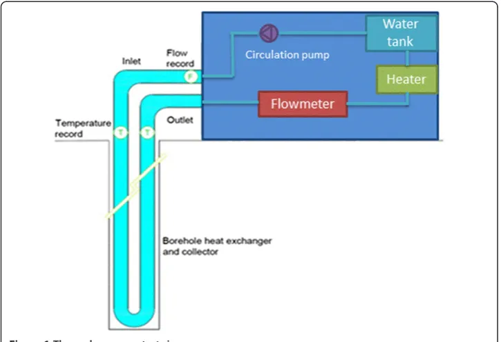
At the current state of technology, the thermal response test (TRT) is thein situtest for the characterization of ground thermal properties with the highest degree of accuracy (Figure 1). It consists of injecting/extracting heat to/from the borehole heat exchanger for a limited time and typically with a constant power flux (Gehlin & Eklof 1996); (Gehlin 2002). During the test, the temperature variation of the circulating fluid is recorded, and through these data, it is possible to measure the equivalent thermal properties of the quasi-cylindrical ring affected by the heat exchanger (Eskilson 1987). The quasi-cylindrical ring is
composed of several materials; some of them are artificial (bentonite, pipes) and have theoretically constant thermal properties, while others, the natural ones, have variable ones.
If the test is run for around 3 days, it is impossible to have a full characterization of the involved area, simply because TRT characterizes only the neighborhood of the heat ex-changer at hand and just for the test duration. In fact, the 3D/2D variability of the thermal properties through the whole reservoir cannot be studied if just one test is available, which is the standard practice. Such variability can be an important concern if a multi-borehole geothermal field has to be implemented. Moreover, the temporal variability of groundwater level could change the equivalent thermal properties of each heat exchanger (Lee and Lam 2012). Nevertheless, TRT is the most adequate, popular, and efficient tool for identifying the parameters to be considered when designing the BTES system.
As a matter of fact, TRT data can be considered as a thermal production test on the studied area. As there is a well-known parallelism between the oil and gas case and groundwater production wells (Raymond et al. 2011) and as it is clear the parallelism be-tween the geothermal heat exchanger and groundwater production wells, we can therefore find a similarity between the oil and gas tests and the thermal response test. In fact, in both cases, we have a sort of production test, which is, for the former, a well test, while for the latter, the TRT. Through these tests, we want to obtain the most important parame-ters for our cases: hydraulic conductivity, porosity, and saturations for the oil and gas case; and ground thermal conductivity, ground volumetric heat capacity, borehole thermal resistance, and undisturbed ground temperature for the geothermal problem.
Starting from these assumptions, it is correct to apply to the shallow geothermal res-ervoirs the same tools and techniques used for fluid resres-ervoirs, tailored on the heat ex-change issue. That is why we adopted the approach of inverse modeling (Mata-Lima 2006) for reservoir characterization, typical of oil and gas field analysis, given the existing similarities. The software used to develop the dynamic simulation is FEFLOW
6.1 (finite element subsurface flow system) (Al-Khoury et al. 2010). In this study, a geostatistical reservoir model has been set up based on the studies on thermal proper-ties and spatial variability hypotheses, and a real TRT has been tested.
Methods
Modelization of an oil reservoir requires the characterization of both the formation field (lithology, permeability, porosity, saturation distribution, etc.) and fluid mobility properties (Mata-Lima 2008). Moreover it requires the knowledge of production data for modeling the internal properties of the reservoir. Normally, in a simple problem of porous flow, a progressive mathematical modeling (forward modeling) is used, in which it is assumed that the underground properties and the initial and boundary conditions are known.
In reality, the information characterizing the entire spatial domain in the considered case does not exist; on the other hand, indirect methods used to obtain data give us sec-ondary information (soft data) that needs a joint validation with primary information (hard data). This information furnishes the spatial distribution of the reservoir properties.
These data, so called static, are not sufficient to characterize the performance of a reservoir; to do that, we have to integrate dynamic data (production data). Landa (1997) distinguishes three groups of methods for the reservoir study:
(1)Probabilistic or stochastic (with static data) (2)Deterministic (with dynamic data)
(3)Emergent (combining previous methods).
If in reservoir engineering, the system is physically inaccessible, emergent methods are used, coupled with inverse modeling to characterize its petrophysical properties. In its general form, an inverse problem refers therefore to the determination of the plaus-ible physical properties of the system, or information about these properties, given the observed response of the system to some stimulus (Oliver et al. 2008).
In a geostatistical approach to the inverse problem, a set fine grid values of permeability and porosity is perturbed in order to match the synthetic response of the model with real production data (Mata-Lima 2008). The biggest advantage of this method is that by perturbing the images (previously created through a geostatistical process as different real-izations of the same variable), we preserve the spatial distribution of the data as revealed by variograms and distributions of the original variables (Hu 2002; Hu et al. 2001).
By applying this technique to the geothermal case, we will create different realizations of thermal conductivity (through a direct sequential simulation; Soares 2001), and we will find which one is the best to fit the real production data (temperature evolution along time). The software used to develop this procedure is FEFLOW 6.1.
The whole process of the inverse problem applied to the shallow geothermal exploitation suffers the problem of lack of thermal conductivity measurements. In fact, up to now, there are no well developed and inexpensive technologies for direct measuring, in laboratory and on site, of ground thermal properties. For rocks, the technology is much further developed. Moreover, the thermal conductivity maps are being developed in few regions.
(1)To give heterogeneity to our reservoir (accurate grids)
(2)To quantify uncertainty through different models with the same heterogeneity (3)To integrate different types of data at different scale and precisions (hard and soft
data) through cokriging and co-simulations.
The resolution method proposed for this kind of problem is an algorithm of inverse modeling whose objective is reservoir characterization by the integration of dynamic data in stochastic modeling using direct sequential simulation (DSS) and co-simulation as a convergent process of global and regional perturbation of the permeability images. This algorithm allows obtaining a spatial distribution of the reservoir permeability which respects both static data (variogram and histogram of permeability distribution in the stochastic model) and dynamic data (flux in the observations boreholes).
The followed procedure requires the following:
(1)Stochastic modeling of the reservoir properties is made by the facies geometry simulation and by the petrophysical properties distribution in the facies exploiting geostatistics
(2)Dynamic modeling of the reservoir fluids, based on energy and mass conservation laws, Darcy law, dynamic models equation (state equation), and relationship between relative permeability and capillary pressure. This simulation model is composed by:
(a) Equation regulating the fluid dynamics (b)Maps to define the study area
(c) Data describing the area and the parameters (d)Initial and boundary conditions.
Creation of the stochastic model of thermal properties
In order to represent the variability of the natural medium, we need to perform geostatistical simulation of the parameters characterizing the soil (Bruno et al. 2011). We decide to neglect the simulation of thermal capacity because its variability is very low, and it does not influence much the dynamic simulation of the reservoir. On the other hand, the thermal conductivity is the most important parameter controlling the dynamic simula-tion, and that is the reason why we will proceed in its geostatistical simulation.
Different are the types of simulation that could be used for the purpose: the chosen one is the direct sequential simulation (Soares 2001). In this simulation, no transform-ation of the original variable into a Gaussian one is needed (in contrast to the sequen-tial Gaussian simulation), which lets us deal with different types of inisequen-tial distributions of the properties. The simulation has the objective of using local averages and variance for resampling the global distribution law.
knowing the average, maximum, and minimum per soil). The software used for running the geostatistical simulation was GeoMS, a geostatistical tool developed by the Centre for Natural Resources and Environment of Instituto Superior Técnico of Lisbon.
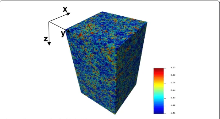
After having run our simulation, we will obtain 60 × 60 × 125 values of the thermal con-ductivity distributed on a Cartesian grid (Figures 4 and 5). In this case, we are considering a real thermal response test that was run on an almost homogeneous soil, made by marl and only 1.5 m of clay at the surface. Unfortunately, we do not have cores; we only have the information about the stratigraphy. Our purpose is to check what would happen if we were using this test to dimension six different boreholes located in the same area: would the performance be different in the other five because of the thermal conductivity variabil-ity? Therefore, the dynamic simulation will be run on six boreholes all in the same area; that is why we needed to extract six columns of data from the simulation, which, from now on, will be considered as real data along the borehole.
After that, the data from the six boreholes were analyzed geostatistically (average, variance, and variogram), and by using them as input, other geostatistical simulations were run (DSS) in order to obtain different realizations from the same thermal con-ductivity data and for the same study area.
Dynamic modeling of thermal response test using FEFLOW
FEFLOW is a dynamic flow simulator that includes also a module for BHE modeling and simulation. In the new version, 6.1, the boundary conditions of BHE were
Table 1 VDI information about thermal conductivity of different type of soils
Sandstone Saturated clay
Dry clay
Limestone Marl Saturated sand
Dry sand
Clay scists
Average 2.3 1.7 0.5 2.8 2.1 2.4 0.4 2.1
Minimum 1.3 0.9 0.4 2.5 1.5 1.7 0.3 1.5
Maximum 5.1 2.3 1 4 3.5 5 0.8 2.1
Variance 1.267 0.467 0.2 0.5 0.67 1.1 0.17 0.2
improved, and they now allow defining directly the inlet temperature (as constant or transient value) and differentials of power or temperature to represent the operation of heat pumps. Moreover, it is possible to create arbitrary connections between the inlet and outlet pipes of the BHEs, both parallel and serial.
The real thermal response test was conducted in the Emilia Romagna region in Italy, close to Rimini; the borehole heat exchanger had a length of 100 m and a diameter of 0.127 m (Table 2). The collector was a double U-tube with an external collector diam-eter of 0.032 m. Water was used as a fluid while the test was running in a cooling mode (injection of heat into the ground).
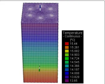
The image of undisturbed ground temperature was obtained by running a natural state simulation (Figure 6), imposing the ground temperature (13.79°C) and the expected temperature at 125-m depth (it was calculated by knowing the average
Figure 3Variogram calculated alongzin order to consider the entire borehole data.There are two nested structures, one nugget effect with 0.1 as sill and the other spherical with sill 0.065 and range 7.4 m.
z
y
x
temperature of the area all over the year and the thermal flow rate from the earth). Moreover, we had the real measured average temperature along the borehole which was 14.3°C that fits our dynamic simulation.
From the stratigraphic point of view, in this case, we have a very simple one:
0 to 1.5-m dry clay with a thermal capacity of 1.6 MJ/m3K
1.5 to 100-m marl with a thermal capacity of 2.25 MJ/m3K (there are some small
infiltrations of water between 60- and 65-m depths).
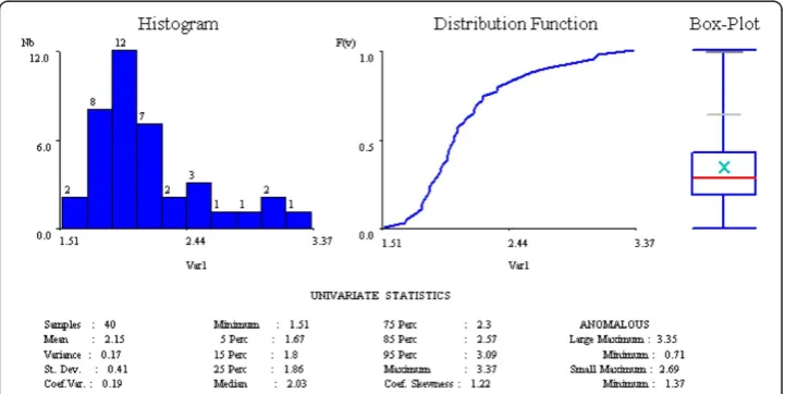
The average inlet temperature of the test was 30.82°C, while that of the average outlet was 27.2°C. As an input for the simulator, we have to enter a reference temperature for Figure 5Histogram and distribution function of the simulated thermal conductivity data and all the elementary statistics.
Table 2 Fluid, grout and borehole properties
BHE Value Fluid Value Grout (bentonitic
mortar)
Value
Type Double
U-tube
Mass density 1000 kg/ m3
Thermal conductivity 0.347 to 0.386 W/ mK
Borehole diameter 0.127 m Thermal conductivity
0.52 W/ m·K
Volumetric thermal capacity
1.704 M J/m3∙K
Length 100 m Specific heat
capacity
4186 J/ kg·K
Density 1420 kg/m3
Outer pipe diameter 0.032 m Dynamic viscosity 0.001 kg/ m·s
Thermal resistance 0.018 to 0.02 m2∙K/W Wall thickness 0.0029 m
Pipe thermal conductivity
0.4 W/m·K
Volume flow rate/ pipe
the test, which is 30°C, an average flow rate which corresponds to 36 m3/day (1,500 l/h of circulating water with Re = 20.248, turbulent flow), and a variable heat input rate (that will be the one used in the real thermal response test).
The FEFLOW model comprises an area of 60 m × 60 m and a depth of 125 m, di-vided into 21 layers, the first 20 of 5-m thickness, while the last one of 25-m thickness (creating the bottom boundary condition for the borehole heat exchanger). The first layer of 1.5 m of clay was neglected in the model, and all the volume was set as marl.
Figure 6Undisturbed ground temperature at timet= 0.Average temperature is 14.6°C.
15 17 19 21 23 25 27 29 31 33
0 20000 40000 60000 80000 100000 120000 140000 160000
T
emp
er
a
tu
re (°C
)
Time (seconds)
Comparison real -simulated TRT curve
real BHE1
The thermal conductivity values for all the different layers were used, the ones obtained by running direct sequential simulations on GeoMS and whose calculations were described in the previous paragraph. There is no groundwater. The BHEs are dis-posed in a circular line inside the domain area; each of them has the same inlet temperature which is the same as that of the thermal response test run. In this way, we will try to reproduce the TRT in different parts of the domain, showing if FEFLOW manages to reproduce a thermal response test and if there are differences in the re-sponse due to the local variability of ground thermal conductivity.
Results and discussion
First of all, it has to be verified how FEFLOW simulation can reproduce a real thermal response test. As it can be seen from Figure 7, it is possible, using the inlet temperature as the variable input, to obtain a reliable reconstruction of the trend of a TRT curve.
The shape of the curve is exactly like what we have in the real TRT, but the temperature shows a systematic difference of almost 1°C between the two curves. The difference between the real curve and the simulated ones oscillates within 4% and 8%; the simulated curve is always higher than the real one. The results obtained with the infinite line source analysis are that the borehole thermal resistance is 0.08 K·m/W, while the ground thermal conductivity is 1.65 W/m·K.
0.040 0.045 0.050 0.055 0.060 0.065 0.070 0.075
1.350 1.370 1.390 1.410 1.430 1.450 1.470 1.490 1.510 1.530 1.550
B o rehol e res istanc e (K· m /W )
Ground thermal conductivity (W/m·K)
Results of the different simulations
Sim 1 Sim 2 Sim 3 Sim 4 Sim 5 Sim 6
Figure 8Sensitivity of results to changing some input parameters.
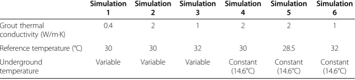
Table 3 Input parameters for the different simulations
Simulation 1 Simulation 2 Simulation 3 Simulation 4 Simulation 5 Simulation 6 Grout thermal conductivity (W/m·K)
0.4 2 1 2 2 1
Reference temperature (°C) 30 30 32 30 28.5 32
Underground temperature
Variable Variable Variable Constant (14.6°C)
Constant (14.6°C)
When comparing the results obtained with different images of thermal conductivity, the difference is very low (less than 1%), and it does not affect the thermal response test curve. As we are considering a homogeneous geology, in this case, it is more interesting to focus on the variation of the curve due to the changes in terms of the borehole characteristics.
Figure 8 shows basically the sensitivity of the results due to changing some of the input parameters. It is rather clear that by changing some parameters in the realization of the borehole heat exchanger, the results change both in the borehole thermal resistance and in the ground thermal conductivity calculations made by using the infinite line source method. As can be seen clearly from Table 3, by changing the grout thermal conductivity (cases 1 and 2) and keeping the same all the other parameters, we obtain different results be-cause of the different borehole thermal resistances linked to the grout conductivity. Be-tween case 2 and case 4, we had only the temperature of the ground changed from a variable (with average of 14.3°C) to a constant one of 14.3°C, and what we experience is a very small difference in the result (less than 1% difference between the resistances and 3% between thermal conductivities), while in cases 3 and 6, in which the only difference lies in the underground temperature, the difference between the result is much higher (less than 3% difference between the resistances and 6% between thermal conductivities). Concerning the difference between cases 4 and 5, by changing only the reference temperature, nothing changes in the results (the borehole thermal resistance and ground thermal conductivity are the same for each borehole in the two cases).
Concluding the remarks about this sensitivity analysis, we can conclude that whether or not we change the reference temperature, the results will remain the same; on the contrary, if we play with the grout thermal conductivity, we will for sure experience a variation in the borehole thermal resistance and in the ground thermal conductivity.
The ground temperature as well influences the result, which means that considering it constant will rather change the results (infinite line source theory considers it con-stant along the borehole length). Therefore, by changing the borehole condition, we
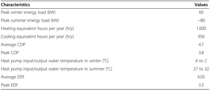
Table 4 Thermal characteristics of a house case study
Characteristics Values
Peak winter energy load (kW) 60
Peak summer energy load (kW) −80
Heating equivalent hours per year (h/y) 1.600
Cooling equivalent hours per year (h/y) 950
Average COP 4.7
Peak COP 3.8
Heat pump input/output water temperature in winter (°C) 6 to 2
Heat pump input/output water temperature in summer (°C) 27 to 32
Average EER 4.05
Peak EER 3.3
Table 5 Results for the house case study
Borehole length (summer) Borehole length (winter)
Case a 1,418 933
Case b 1,488 975
can obtain a different ground thermal conductivity which can lead to some changes in the project. By considering a real case, we can compare in terms of the required bore-hole length how these differences affect the results. Let us consider a house with the thermal characteristics resumed in Table 4.
For the calculation of the borehole length needed, we will refer to the ASHRAE (Atlanta, GA) calculation method. The results are shown in Table 5 for the two extreme cases (a)λ = 1.38 W/mK andRb= 0.06 mK/W and (b)λ = 1.54 W/mK and
Rb= 0.0675 mK/W.
As we can see from this example, the bigger the project, the greater the difference; of course, if we are dealing with a single-house application, there will be a less than 5-m difference for the single borehole needed.
It is, therefore, possible to conclude that the grouting (and then the borehole ther-mal resistance) plays a very important role in the calculation of ground therther-mal con-ductivity, and it has to be taken into account while evaluating the TRT results (Borinaga-Trevino et al. 2013).
Conclusions
This paper has shown that the problem of defining the thermal properties of a shallow geothermal reservoir is a complex one. The traditional methodology for reservoir characterization is simplified because it ignores the space time variability and the linked uncertainties; therefore, for a robust analysis, new probabilistic approaches are needed.
Particularly, in this paper, a geostatistical approach was proposed to get the best image of a ground thermal conductivity for shallow geothermal applications. In practice, an in-verse approach is applied on the case of a thermal response test (which can be seen as a production test in the oil field) in order to get the image of thermal conductivity of the area involved in the test. As the case considered was a very simple one, with homogeneous ground geology, we were only able to verify that there is a good reconstruction of the shape of the thermal response test curve, with all the geostatistical models. Knowing that, a sensitivity study was developed in order to understand which parameter is the one that most influenced the test and how it changes the results. It was seen that one of the most influential parameters is the grout thermal conductivity of the borehole, which can change the results up to a 10% of the ground thermal conductivity from one simulation to an-other. This leads to a 5% difference in the borehole length.
Competing interests
The author declares that she has no competing interests.
Received: 12 June 2013 Accepted: 26 August 2013 Published: 11 September 2013
References
Al-Khoury R, Kolbel T, Schramedei R (2010) Efficient numerical modeling of borehole heat exchangers. Comput Geosci 36:1301–1315
Borinaga-Trevino R, Pascual-Munoz P, Castro-Fresno D, Blanco-Fernandez E (2013) Borehole thermal response and thermal resistance of four different grouting materials measured with a TRT. Appl Therm Eng 53:13–20 Bruno R, Focaccia S, Tinti F (2011) Geostatistical modeling of a shallow geothermal reservoir for air conditioning of
buildings. In: COGeo (ed) Proceeding of IAMG 2011 mathematical geosciences at the crossroads of theory and practice. COGeo, Salzburg
Eskilson P (1987) Thermal analysis of heat extraction boreholes. PhD thesis, Department of Technical Physics, University of Lund, Sweden
Gehlin S (2002) Thermal response test: method development evaluation. PhD thesis, Department of Environmental Engineering, University of Lulea, Sweden
Hu L (2002) Combination of dependent realization within the gradual deformation methods. Mathematical Geology 34(8):953–963
Hu L, Blanc G, Noetinger B (2001) Gradual deformation and iterative calibration of sequential simulations. Mathematical Geology 33(4):475–489
Landa JL (1997) Reservoir parameter estimation constrained to pressure transients, performance history and distributed saturation data. Department of Petroleum Engineering, Stanford University, California
Lee CK, Lam HN (2012) A modified multi-ground-layer model for borehole ground heat exchangers with an inhomogeneous groundwater flow. Energy 47:378–387
Mata-Lima H (2006) Modelação inversa de reservatórios petrolíferos - integração de dados da dinâmica de fluídos na parametrização e upscaling. PhD thesis, Ciências de Engenharia. Instituto Superior Técnico, Universidade Técnica de Lisboa, Portugal
Mata-Lima H (2008) Reservoir characterization with iterative direct sequential co-simulation: integrating fluid dynamic data into stochastic model. Journal of Petroleum Science and Engineering 62:59–72
Oliver DS, Reynolds AC, Liu N (2008) Inverse theory for petroleum reservoir characterization and history matching. Cambridge University Press, UK
Raymond J, Therrien R, Gosselin L, Lefebvre R (2011) A review of thermal response test analysis using pumping test concepts. Groundwater 49(6):932–945
Soares A (2001) Direct sequential simulation and cosimulation. Mathematical Geology 33(8):911–926
Witte HJL, van Gelder AJ (2006) Geothermal response tests using controlled multi-power level heating and cooling pulses (MPL-HCP): quantifying ground water effects on heat transport around a borehole heat exchanger. In: Ecostock conference, Richard Stockton College of New Jersey, USA, 31 May–2 June 2006
doi:10.1186/2195-9706-1-3
Cite this article as:Focaccia:Thermal response test numerical modeling using a dynamic simulator.Geothermal
Energy20131:3.
Submit your manuscript to a
journal and benefi t from:
7Convenient online submission 7Rigorous peer review
7Immediate publication on acceptance 7Open access: articles freely available online 7High visibility within the fi eld
7Retaining the copyright to your article