Volume 2007, Article ID 45962,9pages doi:10.1155/2007/45962
Research Article
Linear Prediction Using Refined Autocorrelation Function
M. Shahidur Rahman1and Tetsuya Shimamura2
1Department of Computer Science and Engineering, Shah Jalal University of Science and Technology, Sylhet 3114, Bangladesh 2Department of Information and Computer Sciences, Saitama University, Saitama 338-8570, Japan
Received 16 October 2006; Revised 7 March 2007; Accepted 14 June 2007
Recommended by Mark Clements
This paper proposes a new technique for improving the performance of linear prediction analysis by utilizing a refined version of the autocorrelation function. Problems in analyzing voiced speech using linear prediction occur often due to the harmonic struc-ture of the excitation source, which causes the autocorrelation function to be an aliased version of that of the vocal tract impulse response. To estimate the vocal tract characteristics accurately, however, the effect of aliasing must be eliminated. In this paper, we employ homomorphic deconvolution technique in the autocorrelation domain to eliminate the aliasing effect occurred due to periodicity. The resulted autocorrelation function of the vocal tract impulse response is found to produce significant improvement in estimating formant frequencies. The accuracy of formant estimation is verified on synthetic vowels for a wide range of pitch frequencies typical for male and female speakers. The validity of the proposed method is also illustrated by inspecting the spectral envelopes of natural speech spoken by high-pitched female speaker. The synthesis filter obtained by the current method is guaran-teed to be stable, which makes the method superior to many of its alternatives.
Copyright © 2007 M. S. Rahman and T. Shimamura. This is an open access article distributed under the Creative Commons Attribution License, which permits unrestricted use, distribution, and reproduction in any medium, provided the original work is properly cited.
1. INTRODUCTION
Linear predictive autoregressive (AR) modeling [1, 2] has been extensively used in various applications of speech pro-cessing. The conventional linear prediction methods, how-ever, have been known to possess various sources of limi-tations [2–4]. These limilimi-tations are mostly observed during voiced segments of speech. Linear prediction method seeks to find an optimal fit to the log-envelop of the speech spec-trum in least squares sense. Since the source of voiced speech is of a quasiperiodic nature, the peaks of linear prediction spectral estimation are highly influenced by the frequency of pitch harmonics (i.e., fundamental frequency,F0). In
high-pitched speaking, such estimation is very difficult due to the wide spacing of harmonics. Unfortunately, in order to study the acoustic characteristics of either the vocal tract or the vo-cal fold, the resonance frequencies of the vovo-cal tract must be estimated accurately. Consequently, researchers long have at-tempted numerous modifications to the basic formulation of linear prediction analysis. While a significant number of techniques for improved AR modeling have been proposed based on the covariance method, improvements on the auto-correlation method are rather few.
Proposals based on the covariance method include an-alyzing only the interval(s) included within a duration of
glottal closure with zero (or nearly zero) excitations [5–7]. However, it is very difficult to find such an interval of ap-propriate length on natural speech especially on speech ut-tered by females or children. Even if such an interval is found, the duration of the interval may be very short. The closed-phase method has been shown to give smooth for-mants contours in cases where the glottal close phase is about 3 milliseconds in duration [6]. If the covariances are com-puted from an extremely short interval, they could be in er-ror, and the resulting spectrum might not accurately reflect the vocal tract characteristics [8]. In [9], Lee considered the source characteristics in the estimation process of AR coef-ficients by weighting the prediction residuals, where more weight is given to the bulk of smaller residuals while down-weighting the small portion of large residuals. A more gen-eral method, of course, was proposed earlier by Yanagida and Kakusho [10] where the weight is a continuous function of the residual. System identification principle [11–14] has also been exploited using least square method where an estimate of input is obtained in the first pass which is then used in the second-pass together with the speech waveform as output. Thus the estimated spectrum is assumed to be free from the influence ofF0. Obtaining a good estimate of the input from
assumptions about glottal waves, Deng et al. [15] estimated glottal waves containing detail information over closed glot-tal phases that yield unbiased estimates of vocal tract filter coefficients. Results presented on sustained vowels are quite interesting.
In an autocorrelation based approach, Hermansky et al. [16] attempt to generate more frequency samples of the original envelope by interpolating between the measured harmonic peaks and then fit an all-pole model to the new sets of frequency points. Motivated by knowledge of the au-ditory system, Hermansky [17] proposed another spectral modification approach that accounted for loudness percep-tion. Vahro and Alku proposed another variation of linear prediction in [18], where instead of treating all thep previ-ous samples of speech waveformx(n) equally, an emphasis is given onx(n−1) than the other samples. High correla-tion between two adjacent samples was the motivacorrela-tion of this approach. The higher formants were shown to be estimated more precisely by the new technique. However, the lower for-mants are well known to be mostly affected by the pitch har-monics.
In this paper, we consider the effect of periodicity of excitation from a signal processing viewpoint. For the lin-ear prediction with autocorrelation (LPA) method, when a segment is extracted over multiple pitch periods, the ob-tained autocorrelation function is actually an aliased version of that of the vocal tract impulse response [3]. This is be-cause copy of the autocorrelation of vocal tract impulse re-sponse is repeated periodically with the periodicity equiva-lent to pitch period, which overlaps and alters the underly-ing autocorrelation function. However, the true solutions of the AR coefficients can be obtained only if the autocorrela-tion sequence equals that of the vocal tract impulse response. This true solutions can be achieved approximately at a large value of pitch period. As the pitch period of high-pitched speech is very short, the increased overlapping causes the low-order autocorrelation coefficients considerably different from those of vocal tract impulse response. This leads to the fact that the accuracy of LPA decreases asF0increases. To
re-alize the true solutions thus the aliasing must be removed. The problem is greatly solved by the discrete-all-pole (DAP) model in [3], where the aliasing is minimized in an iterative way. But it sometimes suffers from spurious peaks between the pitch harmonics. An improvement over DAP has been proposed in [19] where a choice needs to be made depend-ing on whether the signal is periodic, aperiodic, or a mixture of both. This choice and the iterative computing are the dis-advantages of the DAP methods.
As we will see inSection 2, the autocorrelation function of the speech waveform gets aliased due to a convolution operation of the autocorrelation function of vocal tract im-pulse response with that of the excitation im-pulses. The princi-pal problem then is to eliminate the excitation contribution from the aliased version of autocorrelation function of the speech waveform. Homomorphic deconvolution technique [20] has long history of successful applications in separating the periodic component from a nonlinearly combined sig-nal. In this paper, we employ homomorphic deconvolution
method in the autocorrelation domain [21] to separate the contribution of periodicity and thus obtain an estimate of the autocorrelation of vocal tract impulse response which is (nearly) free from aliasing. Unlike DAP methods, the pro-posed solution is noniterative in nature and more straight-forward. Experimental results obtained from both synthetic and natural speech show that the proposed method can pro-vide enhanced AR modeling especially for the high-pitched speech where LPA provides only an approximation.
We organize the paper as follows. We define the problem inSection 2and we propose our method inSection 3. Sec-tions4 and5describe the results obtained using synthetic and natural speeches, respectively. Finally,Section 6is on the concluding remarks.
2. PROBLEMS OF LPA
Though LPA is known to lead an efficient and stable solution of the AR coefficients, this method inherits a different source of limitation. For an AR filter with impulse response:
h(n)=
p
k=1
αkh(n−k) +δ(n), (1)
whereδ(n) is an impulse and pis the order of the filter, the normal equations can be shown as (see [22])
p
k=1
αkrh(i−k)=rh(i), 1≤i≤p, (2)
whererh(i) is the autocorrelation function ofh(n). For a pe-riodic waveforms(n), (2) can be expressed as
p
k=1
αkrn(i−k)=rn(i), 1≤i≤p, (3)
wherern(i) is the autocorrelation function of the windowed
s(n) (s(n) is constructed to simulate voiced speech by con-volving a periodic impulse train withh(n)).
For such periodic signal, El-Jaroudi and Makhoul [3] have shown that rn(i) equals the recurring replicas of rh(i) as given by
r(i)=
∞
l=−∞
rh(i−lT), ∀l, (4)
whereT is the period of excitation andrn(i) can be consid-ered as an equivalent of r(i) for a finite-length speech seg-ment. The effect of T onrn(i) is shown in Figure 1. When the value ofTis large, the overlapping is insignificant; iden-tical values of rh(i) (Figure 1(a)) and rn(i) (Figure 1(b) at
−1 0 1
−25 −20 −15 −10 −5 0 5 10 15 20 25 Time (ms)
A
m
plitude
(a)
−1 0 1
−25 −20 −15 −10 −5 0 5 10 15 20 25 Time (ms)
A
m
plitude
(b)
0 1
−25 −20 −15 −10 −5 0 5 10 15 20 25 Time (ms)
A
m
plitude
(c)
Figure1: Aliasing in the autocorrelation function. (a) Autocorre-lation of the vocal tract impulse response,rh(i); (b) autocorrelation
of a periodic waveform atT =12.5 milliseconds (atF0 =80 Hz); (c) autocorrelation of a periodic waveform atT =4 milliseconds (atF0=250 Hz).
3. HOMOMORPHIC DECONVOLUTION IN THE AUTOCORRELATION DOMAIN
FromSection 2, it is now obvious that true solutions can be obtained only if the autocorrelation function in the normal equations equalsrh(i). In this section, we propose a straight-forward way to derive an estimate of rh(i) from its aliased counterpartrn(i).
We can write (4) as
r(i)=rh(i)∗rp(i), (5)
where∗stands for convolution andrp(i) is the autocorrela-tion funcautocorrela-tion of the impulse train, which is also periodic with periodT. Thus,r(i) is a speech-like sequence and homomor-phic deconvolution technique can separate the component
rh(i) from the periodic componentrp(i). This requires trans-forming a sequence to its cepstrum. The (real) cepstrum is defined by the inverse discrete Fourier transform (DFT) of the logarithm of the magnitude of the DFT of the input se-quence. The resulting equation for the cepstrum of the
au-−1
−0.5 0 0.5 1
A
m
plitude
0 1 2 3 4 5 6
Time (ms) rn
Estimatedrh Truerh
Figure2: Autocorrelation function of vocal tract impulse response and that of windowed speech waveform.
tocorrelation function rn(i) corresponding to a windowed speech segment is given as
crn(i)=N1 N−1
k=0
logRn(k)ej(2π/N)ki, 0≤i≤N−1,
(6)
where Rn(k) is the DFT ofrn(i) andN is the DFT size. A 1024-point DFT is used for the simulations in this paper. It is noted that the termRn(k) is an even function (i.e.,Rn(1 :
N/2)=Rn(N−1 :N/2 + 1)).
The term log|Rn(k)|in (6) can be expressed using (5) as logRn(k)=logRh(k)Rp(k)
=logRh(k)+ logRp(k)
=Crh(k) +Cr p(k).
(7)
Thus an inverse DFT operation on log|Rn(k)|separates the contribution of the autocorrelation function of the vocal tract and source in the cepstrum domain. The contribution ofrh(i) on the cepstrumcrn(i) can now be obtained by mul-tiplying the real cepstrum by a symmetric windoww(i):
crh(i)=w(i)crn(i). (8)
Application of an inverse cepstrum operation to crh(i) converts it back to the original autocorrelation domain. The resulting equation for the inverse cepstrum is given as
rh(i)=N1 N−1
k=0
expCrh(k)ej(2π/N)ki, 0≤i≤N−1,
(9)
Speech
x AC funct.Calculate rn rh∗rp
Cepstrum analysis
Low-time gating
crh+cr p Inv. ceps. analysis
crh rh Levinson
algorithm AR coeff. Deconvolution
Figure3: Block diagram of the proposed method.
−50
−40
−30
−20
−10 0
A
m
plitude
0 1000 2000 3000
Frequency (Hz) True
LPRA LPA
(a)
−50
−40
−30
−20
−10 0
A
m
plitude
0 1000 2000 3000
Frequency (Hz) True
LPRA LPA
(b)
Figure4: Spectra obtained using the autocorrelation sequence in Figures1(b)and1(c): (a) atF0=80 Hz; (b) atF0=250 Hz.
As an example, the deconvolution of the autocorrelation sequence inFigure 1(c)is shown inFigure 2. It is seen that the refined version of the autocorrelation functionrh(i) (thin solid line) obtained through deconvolvolution ofrn(i) is in-deed a good approximation of the autocorrelation function of the true impulse responserh(i) (thick solid line).
The overall method of improved linear prediction us-ing refined autocorrelation (LPRA) function is outlined in the block diagram of Figure 3. Real cepstrum is computed from the autocorrelation function rn(i) of the windowed speech waveform. The low-time gating (i.e., truncation of the cepstral coefficients residing in an interval less than a pitch period) of the cepstrum followed by an inverse cepstral transformation produces the refined autocorrelation func-tionrh(i), which closely approximates the true autocorrela-tion coefficients especially in lower lags that are the most im-portant for formant analysis with linear prediction.
The LPA and LPRA spectral envelopes obtained using the autocorrelation sequence in Figures 1(b) and 1(c) (at
F0 =80 and 250 Hz) are plotted in Figures4(a) and4(b),
respectively, together with the true spectrum. The frequen-cies/bandwidths of the three formants in the “true” spec-trum are (400/80, 1800/140, 2900/240) Hz. Both the LPA and LPRA methods produce perfect spectra at F0 =80 Hz
(as overlapped with the “true” spectrum in Figure 4(a)). AtF0 =250 Hz, however, the LPA spectrum, especially the
first formant frequency and bandwidth, is considerably de-viated from the “true” spectrum, where the spectrum esti-mated using the refined version of the autocorrelation
func-tion atF0 = 250 Hz closely approximates the “true”
spec-trum (inFigure 4(b)). The formant frequencies/bandwidths estimated using LPA and LPRA spectra at F0 = 250 Hz
are (431/170, 1773/123, 2907/304) and (399/94, 1811/142, 2894/256) Hz, respectively.
Though impulse train used in the above demonstration does not exactly represent the glottal volume velocity, the ex-ample is a good representative to show the goodness of the method. InSection 4, we present the results in more detail taking the glottal and lip radiation effects into account.
3.1. Cepstral window selection
which may widen the formant peaks. If the application of in-terest is known a priori (or based on a logic derived from estimated F0s), using two different cepstral windows, one
for analyzing the male speech and the other for the female speech, is more rational. In that case, 3.6 milliseconds and 2.4 milliseconds (36 and 24 cepstral coefficients in case of 10 kHz sampling rate) cepstral windows are good approx-imations for male (supposing F0 ≤ 200 Hz) and female
speeches (supposingF0>200 Hz), respectively.
Detail results on synthetic speech using two fixed-length cepstral windows (according to theF0value of the underlying
signal) are presented inSection 4.
3.2. Stability of the AR filter
The standard autocorrelation functionrn(i) is well known to produce stable AR filter [26,27]. Thus, if the refined version of autocorrelation sequencerh(i) can be shown to retain the property of rn(i), it can be said that the AR filter resulted by the LPRA method is stable. Sincern(i) is real, log mag-nitude of its Fourier transform, log|Rn(k)|at the right-hand side of (6), is also real and even. Thus, the DFT operation following log|Rn(k)|is essentially a cosine transformation. Then, the symmetric cepstral window (for low-time gating) followed by a DFT operation retains the nonnegative prop-erty of log|Rn(k)|in Crh(k) of (9). An estimate of the re-fined autocorrelation sequence (rh(i)) derived from the pos-itive spectrumCrh(k) therefore produces a positive semidef-inite matrix likern(i) [26], which guarantees the stability of the resulting AR filter.
4. RESULTS ON SYNTHETIC SPEECH
The proposed LPRA method is applied for estimating the for-mant frequencies of five synthetic Japanese vowels with vary-ingF0values. The Liljancrant-Fant glottal model [28] is used
to simulate the source which excites five formant resonators [29] placed in series. The filter (1−z−1) is operated on the
output of the synthesizer to simulate the radiation character-istics from lip. The synthesized speech is sampled at 10 kHz. To study the variations of formant estimation against varying
F0, all the other parameters of the glottal model (open phase,
close phase, and slope ratio) are kept constant. The formant frequencies used for synthesizing the vowels are shown in Table 1. Bandwidths of the five formants of all the five vow-els are set fixed to 60, 100, 120, 175, and 281 Hz, respectively. The analysis order is set to 12. A Hamming window of length 20 milliseconds is used. The speech is preemphasized by a fil-ter (1−z−1) before analysis. A 1024-point DFT is used for
cepstral analysis.
4.1. Accuracy in formant frequency estimation
Formant values are obtained from the AR coefficients by using the root-solving method. In order to obtain a well-averaged estimation of the formants, analysis is conducted on twenty different window positions. The arithmetic mean of all the results is taken as a formant value.
Table1: Formant frequencies used to synthesize vowels.
vowel F1 F2 F3 F4 F5Hz
/a/ 813 1313 2688 3438 4438
/i/ 375 2188 2938 3438 4438
/u/ 375 1063 2188 3438 4438
/e/ 438 1813 2688 3438 4438
/o/ 438 1063 2688 3438 4438
The relative estimation error (REE),EFi, of theith for-mant is calculated by averaging the individualFierrors of all the five vowels. Thus we can expressEFias:
EFi= 15
5
j=1
Fij−FijFij, (10)
whereFijdenotes theith formant frequency of thejth vowel andFijis the corresponding estimated value.
Finally, the REE of the first three formants of all the five vowels are summarized as follows:
E= 1
15
5
j=1 3
i=1
Fij−FijFij. (11)
As mentioned earlier inSection 3.1, two fixed length cep-stral windows of length 3.6 milliseconds and 2.4 milliseconds are used to estimate formant frequencies forF0≤200 Hz and
F0>200 Hz, respectively. The REEs of the first, second, and
first three formants estimated using LPA, DAP, and LPRA methods are shown inFigure 5. The code for DAP has been obtained from an open source MATLAB library for signal processing:http://www.sourceforge.net/projects/matsig. The code has been verified to work correctly.
The first and second formants are mostly affected byF0
variations at higherF0s (because of increased aliasing in the
autocorrelation function). It is seen that REE ofF1estimated
using LPA can exceed 15% depending onF0s. Since LPRA
re-duces aliasing in the autocorrelation function occured due to the periodicity of voiced speech, this method results in very smaller REE and affected slightly by theF0 variations. The
DAP modeling results in much accurate estimation of second and third formants, but accuracy of first formant estimation suffers from large errors. The normalized formant frequency error averaged over all the pitch frequencies for each vowel separately is shown inTable 2.
FromTable 2, it is obvious that the LPRA technique pro-posed in this paper can be useful in reducing aliasing effects occurred due to the excitation in the autocorrelation func-tion.
4.2. Dependency on the length of analysis window
0 5 10 15 20
REE
o
f
F1
(%)
100 150 200 250 300 350
Fundamental frequency,F0(Hz)
LPA LPRA DAP
(a)
0 1 2 3 4
REE
o
f
F2
(%)
100 150 200 250 300 350
Fundamental frequency,F0(Hz)
LPA LPRA DAP
(b)
0 2 4 6 8
REE
o
f
F1
,
F2
and
F3
(%)
100 150 200 250 300 350
Fundamental frequency,F0(Hz)
LPA LPRA DAP
(c)
Figure5: Relative estimation error (REE) of formant frequencies: (a) REE ofF1; (b) REE ofF2; (c) REE ofF1,F2, andF3together.
of LPRA has changed significantly (with respect to the re-sults obtained using 20- milliseconds frame inFigure 5(a)) as compared with that of LPA method. For longer analysis window, the increase in the correlation coefficients at the pitch-multiples result in larger cepstral coefficients around the pitch lags. Thus the convolution effect gets stronger for longer window. The dependency of cepstral deconvolution on window length has been discussed in [25] where it is shown that better deconvolution takes place when the frame length is about three pitch periods. A 40- milliseconds long
0 5 10 15
REE
o
f
F1
(%)
100 150 200 250 300 350
Fundamental frequency,F0(Hz)
LPA DAP LPRA
Figure 6: REE of first formant frequency when frame size is 40 milliseconds.
0 20 40 60 80 100 120 140
Band
w
idth
er
ror
(Hz)
100 150 200 250 300 350
Fundamental frequency,F0(Hz)
LPA LPRA DAP
Figure7: Bandwidth error of first three formants.
frame extracted from 250- Hz pitch speech signal contains ten pitch periods of signal which is much longer than the ex-pected length.
4.3. Accuracy in formant bandwidth estimation
The absolute difference between the actual and estimated bandwidths averaged over the first three formant bandwidths is shown in Figure 7. Bandwidths are estimated in a simi-lar way as formant frequencies. Though the improvement in estimating formant bandwidths is not as significant as that achieved in formant frequencies, it still shows nice improve-ments for high-pitched speakers as compared to other meth-ods.
5. RESULTS ON REAL SPEECH
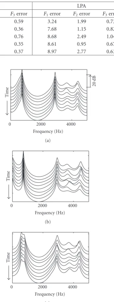
Performance of the proposed method on natural speech is demonstrated in Figures8and9, where we show the spectral envelopes obtained from several voiced segments. The speech materials used in Figures8(a),8(b), and8(c)are extracted from vowel sound /a/ atF0=300 Hz, from /o/ in CV sound
/bo/ atF0=250 Hz, and from /ea/ in /bead/ atF0=256 Hz,
Table2: Normalized formant error (in %) for each vowel.
Method LPRA DAP LPA
Vowel F1error F2error F3error F1error F2error F3error F1error F2error F3error
/a/ 2.13 1.30 0.42 1.05 1.47 0.59 3.24 1.99 0.73
/i/ 3.08 0.51 0.45 8.22 0.67 0.36 7.68 1.15 0.82
/u/ 2.81 1.33 0.60 8.05 1.32 0.76 8.68 2.49 1.04
/e/ 2.86 0.48 0.46 6.19 0.69 0.35 8.61 0.95 0.67
/o/ 2.94 1.38 0.42 2.04 0.96 0.37 8.97 2.77 0.63
0 1000 2000 3000 4000 5000 Frequency (Hz)
20
dB
DAP LPRA LPA
(a)
0 1000 2000 3000 4000 5000 Frequency (Hz)
DAP LPRA LPA
(b)
0 1000 2000 3000 4000 5000 Frequency (Hz)
DAP LPRA LPA
(c)
Figure8: Analysis of natural voiced segments (a) from /a/ atF0 = 300 Hz; (b) from /o/ in /bo/ atF0=250 Hz; (c) from /ea/ in /bead/ atF0=256 Hz.
the LPA spectra, especially the lower, formants are not re-solved with accurate bandwidths. The second formant band-width in Figure 8(a) is widened, while it is constricted in Figure 8(b). The second and third formants in LPA spec-trum of Figure 8(c) remain unresolved. The LPA spectral estimation is affected due to the inclusion of pitch infor-mation with vocal tract filter coefficients. The LPRA
spec-0 2000 4000
Frequency (Hz)
20
dB
Ti
m
e
(a)
0 2000 4000
Frequency (Hz)
Ti
m
e
(b)
0 2000 4000
Frequency (Hz)
Ti
m
e
(c)
Figure9: Analysis of natural vowel /o/ atF0 =352 Hz (a) using LPA method; (b) using DAP method; (c) using LPRA method.
tra, on the other hand, exhibit accurate formant peaks in all the cases where the influence due to the pitch harmon-ics is not significant. The DAP spectrum in Figure 8(a) is estimated well, but the spectra in Figures8(b)and8(c)are more or less identical with the LPA spectra. Running spec-tra estimated from a prolonged vowel sound /o/ at very high pitch (F0=352 Hz) using the LPA, DAP, and LPRA methods
improvement obtained by the current method is obvious in Figure 9, where the closely located lower formants (first and second) are perfectly estimated in the LPRA spectra. These examples indicate the reduction of aliasing in the autocor-relation function achieved through the deconvolution mea-sure.
6. CONCLUSION
In this paper, we proposed an improvement to the linear pre-diction with autocorrelation method for spectral estimation. The autocorrelation function of voiced speech is distorted by the periodicity in a convolutive manner which can greatly be removed using the homomorphic filtering approach. The method works noniteratively and is suitable for analyzing high-pitched speech. The standard cepstral analysis [20] em-ployed here, of course, introduces some distortion due to windowing and cepstral truncation. Use of an improved de-convolution method that takes the windowing effects into ac-count (e.g., [25]) can compensate the problem. Furthermore, the straightforward deconvolution method does not account for the time-varying glottal effects. Thus, the performance of the LPRA method can be improved by eliminating the effects due to glottal variations [15].
One of the greatest concerns for speech synthesis is the stability of the linear prediction synthesis filter. Unfortu-nately, most of the well-known methods [6, 7, 9–11, 14] emerged so far for analyzing high-pitched speech are based on covariance method which cannot guarantee the stability of the resulted AR filter. The proposed method, on the other hand, is guaranteed to produce a stable synthesis filter.
ACKNOWLEDGMENT
The authors are thankful to the three anonymous reviewers for their thorough and insightful comments on the manu-script.
REFERENCES
[1] B. S. Atal and S. L. Hanauer, “Speech analysis and synthesis by linear prediction of the speech wave,”The Journal of the Acous-tical Society of America, vol. 50, no. 2B, pp. 637–655, 1971. [2] J. Makhoul, “Linear prediction: a tutorial review,”Proceedings
of the IEEE, vol. 63, no. 4, pp. 561–580, 1975.
[3] A. El-Jaroudi and J. Makhoul, “Discrete all-pole modeling,”
IEEE Transactions on Signal Processing, vol. 39, no. 2, pp. 411– 423, 1991.
[4] G. K. Vallabha and B. Tuller, “Systematic errors in the for-mant analysis of steady-state vowels,”Speech Communication, vol. 38, no. 1-2, pp. 141–160, 2002.
[5] D. Y. Wong, J. D. Markel, and A. H. Gray Jr., “Least squares glottal inverse filtering from the acoustic speech waveform,”
IEEE Transactions on Acoustics, Speech, and Signal Processing, vol. 27, no. 4, pp. 350–355, 1979.
[6] A. Krishnamurthy and D. G. Childers, “Two-channel speech analysis,”IEEE Transactions on Acoustics, Speech, and Signal Processing, vol. 34, no. 4, pp. 730–743, 1986.
[7] Y. Miyoshi, K. Yamato, R. Mizoguchi, M. Yanagida, and O. Kakusho, “Analysis of speech signals of short pitch period by a sample-selective linear prediction,”IEEE Transactions on Acoustics, Speech, and Signal Processing, vol. 35, no. 9, pp. 1233–1240, 1987.
[8] N. B. Pinto, D. G. Childers, and A. L. Lalwani, “Formant speech synthesis: improving production quality,”IEEE Trans-actions on Acoustics, Speech, and Signal Processing, vol. 37, no. 12, pp. 1870–1887, 1989.
[9] C.-H. Lee, “On robust linear prediction of speech,” IEEE Transactions on Acoustics, Speech, and Signal Processing, vol. 36, no. 5, pp. 642–650, 1988.
[10] M. Yanagida and O. Kakusho, “A weighted linear prediction analysis of speech signals by using the given’s reduction,” in
Proceedings of the IASTED International Symposium on Ap-plied Signal Processing and Digital Filtering, pp. 129–132, Paris, France, June 1985.
[11] Y. Miyanaga, N. Miki, N. Nagai, and K. Hatori, “A speech anal-ysis algorithm which eliminates the influence of pitch using the model reference adaptive system,” IEEE Transactions on Acoustics, Speech, and Signal Processing, vol. 30, no. 1, pp. 88– 96, 1982.
[12] H. Fujisaki and M. Ljungqvist, “Estimation of voice source and vocal tract parameters based on ARMA analysis and a model for the glottal source waveform,” inProceedings of IEEE Inter-national Conference on Acoustics, Speech, and Signal Processing (ICASSP ’87), pp. 637–640, Dallas, Tex, USA, April 1987. [13] W. Ding and H. Kasuya, “A novel approach to the estimation
of voice source and vocal tract parameters from speech sig-nals,” inProceedings of the 4th International Conference on Spo-ken Language Processing (ICSLP ’96), vol. 2, pp. 1257–1260, Philadelphia, Pa, USA, October 1996.
[14] M. S. Rahman and T. Shimamura, “Speech analysis based on modeling the effective voice source,”IEICE Transactions on In-formation and Systems, vol. E89-D, no. 3, pp. 1107–1115, 2006. [15] H. Deng, R. K. Ward, M. P. Beddoes, and M. Hodgson, “A new method for obtaining accurate estimates of vocal-tract filters and glottal waves from vowel sounds,”IEEE Transactions on Audio, Speech, and Language Processing, vol. 14, no. 2, pp. 445– 455, 2006.
[16] H. Hermansky, H. Fujisaki, and Y. Sato, “Spectral envelope sampling and interpolation in linear predictive analysis of speech,” in Proceedings of IEEE International Conference on Acoustics, Speech, and Signal Processing (ICASSP ’84), vol. 9, pp. 53–56, San Diego, Calif, USA, 1984.
[17] H. Hermansky, “Perceptual linear predictive (PLP) analysis of speech,”Journal of the Acoustical Society of America, vol. 87, no. 4, pp. 1738–1752, 1990.
[18] S. Varho and P. Alku, “Separated linear prediction—a new all-pole modelling technique for speech analysis,”Speech Commu-nication, vol. 24, no. 2, pp. 111–121, 1998.
[19] P. Kabal and B. Kleijn, “All-pole modelling of mixed excita-tion signals,” inProceedings of IEEE International Conference on Acoustics, Speech, and Signal Processing (ICASSP ’01), vol. 1, pp. 97–100, Salt Lake City, Utah, USA, May 2001.
[20] A. Oppenheim and R. Schafer, “Homomorphic analysis of speech,” IEEE Transactions on Audio and Electroacoustics, vol. 16, no. 2, pp. 221–226, 1968.
Systems (ISCAS ’05), vol. 3, pp. 2855–2858, Kobe Japan, May 2005.
[22] T. F. Quatieri,Discrete-Time Speech Signal Processing: Princi-ples and Practice, Prentice-Hall, Upper Saddle River, NJ, USA, 2002.
[23] J. S. Lim, “Spectral root homomorphic deconvolution system,”
IEEE Transactions on Acoustics, Speech, and Signal Processing, vol. 27, no. 3, pp. 223–233, 1979.
[24] T. Kobayashi and S. Imai, “Spectral analysis using generalised cepstrum,”IEEE Transactions on Acoustics, Speech, and Signal Processing, vol. 32, no. 6, pp. 1235–1238, 1984.
[25] W. Verhelst and O. Steenhaut, “A new model for the short-time complex cepstrum of voiced speech,”IEEE Transactions on Acoustics, Speech, and Signal Processing, vol. 34, no. 1, pp. 43–51, 1986.
[26] S. M. Kay,Modern Spectral Estimation: Theory and Application, Prentice-Hall, Upper Saddle River, NJ, USA, 1988.
[27] P. Stoica and R. L. Moses,Introduction to Spectral Analysis, Prentice-Hall, Upper Saddle River, NJ, USA, 1997.
[28] G. Fant, J. Liljencrants, and Q. G. Lin, “A four parameter model of glottal flow,” Quarterly Progress and Status, pp. 1– 13, Speech Transmission Laboratory, Royal Institute of Tech-nology, Stockholm, Sweden, October-December 1985. [29] D. H. Klatt, “Software for a cascade/parallel formant