Extended methods for influence
maximization in dynamic networks
Tsuyoshi Murata
*and Hokuto Koga
Background
Diffusion of rumors (or information) can be represented as information propagation in a social network where its nodes are people and its edges are contacts among the peo-ple. The scale of information propagation depends on where to start the propagation. In order to propagate as much as possible, starting nodes should be carefully selected. Selecting starting nodes for large-scale information propagation is important as one of the methods for viral marketing.
Abstract
Background: The process of rumor spreading among people can be represented as information diffusion in social network. The scale of rumor spread changes greatly depending on starting nodes. If we can select nodes that contribute to large-scale diffusion, the nodes are expected to be important for viral marketing. Given a network and the size of the starting nodes, the problem of selecting nodes for maximizing infor-mation diffusion is called influence maximization problem.
Methods: We propose three new approximation methods (Dynamic Degree Discount, Dynamic CI, and Dynamic RIS) for influence maximization problem in dynamic net-works. These methods are the extensions of previous methods for static networks to dynamic networks.
Results: When compared with the previous methods, MC Greedy and Osawa, our proposed methods were found better than the previous methods: Although the performance of MC greedy was better than the three methods, it was computationally expensive and intractable for large-scale networks. The computational time of our pro-posed methods was more than 10 times faster than MC greedy, so they can be com-puted in realistic time even for large-scale dynamic networks. When compared with Osawa, the performances of these three methods were almost the same as Osawa, but they were approximately 7.8 times faster than Osawa.
Conclusions: Based on these facts, the proposed methods are suitable for influ-ence maximization in dynamic networks. Finding the strategies of choosing a suitable method for a given dynamic network is practically important. It is a challenging open question and is left for our future work. The problem of adjusting the parameters for Dynamic CI and Dynamic RIS is also left for our future work.
Keywords: Influence maximization problem, Dynamic networks, SI model
Open Access
© The Author(s) 2018. This article is distributed under the terms of the Creative Commons Attribution 4.0 International License (http://creat iveco mmons .org/licen ses/by/4.0/), which permits unrestricted use, distribution, and reproduction in any medium, provided you give appropriate credit to the original author(s) and the source, provide a link to the Creative Commons license, and indicate if changes were made.
RESEARCH
*Correspondence: [email protected] Department of Computer Science, School
From given network, selecting such starting nodes for large-scale information
prop-agation was formalized as “influence maximization problem” by Kempe et al. [1]. The
original formalization is for static networks. However, nodes and edges can be newly added or deleted in many real social networks. Therefore, influence maximization prob-lem in dynamic networks should be considered. Habiba et al. defined the probprob-lem for dynamic networks [2]. Since the problem was proved to be NP-Hard, computing the best solution in realistic time is computationally intractable. Therefore, many approximation methods based on Monte-Carlo simulation and heuristic methods have been proposed. Methods based on Monte-Carlo simulation are accurate but computationally expensive. On the other hand, heuristic methods are fast but they are less accurate.
In order to find better solutions for the information maximization problem, we pro-pose three new methods for dynamic networks as the extension of the methods for static networks. Dynamic Degree Discount is a heuristic method based on node degree. Dynamic CI is a method based on a node’s degree and the degrees of reachable nodes from the node within specific time. Dynamic RIS uses many similar networks generated by random edge removal. We compare the proposed methods with previous methods. The number of propagated nodes based on our method is about 1.5 times of that of pre-vious methods. And computational time of our method is about 7.8 times faster than previous methods.
The authors discuss the extended methods for influence maximization in dynamic net-works [3]. In addition to the contents in [3], this paper includes detailed explanation of background knowledge, discussions of the effect of different values of parameters in the proposed methods, and detailed analysis of the advantages and disadvantages of the pro-posed methods.
The structure of this paper is as follows. “Related work” section shows related work. “Proposed methods” section presents proposed methods (Dynamic Degree Discount,
Dynamic CI and Dynamic RIS), “Experiments” section explains our experiments, and
“Experimental results” section shows the experimental results. “Discussion” section
shows discussions about the experimental results, and “Conclusion” section concludes
the paper.
Related work
Model of information propagation
We use SI model as the model of information propagation on networks. In SI model, each node in networks is either in state S (susceptible) or in state I (infected). Nodes in state S do not know the information and those in state I know the information. At the beginning of information propagation (at time t=1 ), a set of nodes in state I is fixed as the seed nodes. For all edges (t, u, v) at time t=1, 2,. . .,T , the following operations are performed. If node u is in state I and node v in state S, information is propagated from
u to v with probability , which means the state of v is changed from S to I at time t+1 .
Probability is the parameter of susceptibility, and it controls the percentage of informa-tion propagainforma-tion. At time t=T +1 , information propagation is terminated.
Based on the above notations, we can formulate influence maximization problem as follows. We define σ (S) as the expected number of nodes of state I at time T +1 when
model. (Please keep in mind that S in σ (S) is a set of seed nodes, and S in SI model is sus-ceptible state.) Influence maximization problem in a dynamic network is to search for a set of seed nodes S of size k that maximizes σ (S) when a dynamic network G, duration of the network T, susceptibility of SI model , and the size of seed nodes k are given.
Problems related to influence maximization in dynamic networks
There are some problems related to influence maximization in dynamic networks. Instead of giving item (or information) to seed nodes for free, revenue maximization [4] is the problems of finding seed customers (nodes) and offering discounts to them in order to increase total revenue. Although the problem is important in the field of mar-keting, it is more complicated than influence maximization problem since seed nodes are not treated as equal, and the amount of discount for each node may not be equal. The number of possible parameters increases greatly especially in the case of dynamic networks. Although revenue maximization is one of the important research directions, it is different from influence maximization problem.
Opinion formation [5–7] is another problem related to influence maximization prob-lem. Each agent (node) has an opinion which might be a continuous or a discrete quan-tity. The underlying network represents the society where the agents have interactions. Each agent has an opinion in the society that is influenced by the society. Analyzing the increase and decrease of each opinion is important for modeling the dynamics of opin-ion formatopin-ion and for opinopin-ion polarizatopin-ion [8].
It is often pointed out that the properties of dynamic networks are quite different from those in static networks. Braha and Bar-Yam [9, 10] pointed out the overlap of the cen-trality in dynamic networks and that in the aggregated (static) network is very small. Hill and Braha [11] propose dynamic preferential attachment mechanism that reproduce
dynamic centrality phenomena. Holme presents good surveys on dynamic networks [12,
13].
Influence maximization methods for static networks
Jalili presents a survey on spreading dynamics of rumor and disease based on centrality [14]. There are roughly three approaches for influence maximization problem in static networks. The first is Monte-Carlo simulation methods, the second is heuristic-based methods, and the third is the methods to generate a large number of networks with ran-dom edge removal and select seed nodes based on the generated networks.
Monte-Carlo simulation method is proposed by Kempe et al. [1]. σ (S) is estimated by repeating Monte-Carlo simulation in Kepme’s method. When S is given as a set of seed
nodes, simulations of information propagation are repeated R times and the average
number of infected nodes is defined as σ (S) . Next, the node v which maximizes the dif-ference σ (S∪ {v})−σ (S) is added to seed nodes greedily based on the estimated σ (S) . This operation is repeated until |S| =k.
Since σ (·) is a monotonic and submodular function, when we denote strict solution
of seed nodes as S∗ , the seed nodes obtained by the above greedy algorithm S
greedy
computational cost for finding seed nodes with this method is high, it is not possible to find seed nodes in realistic time for large-scale networks.
Heuristic methods are proposed in order to search for seed nodes at high speed. Chen et al. [15] proposes PMIA to find seed nodes focusing on the paths with high informa-tion propagainforma-tion ratio. Jiang et al. [16] proposed SAEDV which searches for seed nodes by annealing method to obtain σ (·) from adjacent nodes in seed nodes. Chen et al. [17] proposed Degree Discount based on node degree where the nodes adjacent to already selected node are given penalty. This is because when node v is selected as one of seed nodes and u is its neighbor, it is highly likely that v propagates information to u, so selecting nodes other than u as seed nodes is better for information diffusion.
Algorithm of Degree Discount is shown as follows. ti in the algorithm shows the pen-alty of node i. ddi is the degree of node i after giving penalty. ddi is smaller when the value of ti is bigger.
Morone et al. [18] proposed a method for finding seed nodes considering the
degrees of distant nodes. The method calculates the following CIl(v) for each node
and selects seed nodes based on the values:
∂Ball(v, l) in the above formula represents nodes where the distance from node
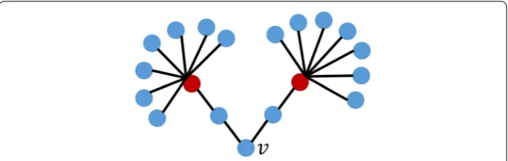
v is l. The example of CIl(v) is explained in Fig. 1. ∂Ball(v, 2) when l=2 are two red
CIl(v)=(kv−1)
u∈∂Ball(v,l)
nodes with distance 2 from node v and the degrees of both nodes are 8. Therefore, CI2(v)=(2−1)× {(8−1)+(8−1)} =14.
The degree of node v itself is low in the network in Fig. 1, but the node v is effec-tive for information propagation because it is connected with some high degree nodes with distance two. This method thus selects seed nodes with wider propagation com-pared with the cases when seed nodes are selected based on the degree of node v only. These heuristic methods compute seed nodes faster than the methods based on Monte-Carlo simulation. However, it is experimentally confirmed that the scale of propagation of the methods depends on network structures and parameters.
Ohsaka et al. [19] proposed a method to generate many networks with random edge
removal in order to solve this problem. Ohsaka’s method is based on “coin flip”
men-tioned in Kempe’s paper [1]. Distribution of nodes where information is propagated
from seed nodes S in static network G is set as DG(S) . And distribution of nodes where
information is propagated from seed nodes S on network where edges are removed at
constant ratio from the network G is set as DG′ (S) . “Coin flip” means that DG(S) equals to D′
G(S) in this situation, and that σ (·) can be estimated by generating many networks with edges removed at constant ratio, not by repeating Monte-Carlo simulation.
Ohsa-ka’s method estimates σ (·) by acquiring Strongly Connected Component (SCC) in each
network generated by RR numbers of networks with edges removed at constant ratio.
SCC is a subgraph where each node in the subgraph can be reachable to and from any other nodes.
Borgs et al. [20] and Tang et al. [21] also propose methods similar to Ohsaka’s method. The difference from Ohsaka’s method is σ (·) , which is not estimated directly
from generated networks. Reachable nodes from randomly selected node v are
com-puted, and then seed nodes are selected based on the nodes. More specifically, the algorithm is as follows.
There are other approaches for influence maximization problem in different prob-lem settings. Chen et al. [22] proposed a method to solve the problem with time limit. Feng et al. [23] solves the influence maximization problem in a situation where fresh-ness of the information degrades as it spreads. Mihara et al. [24] proposed a method to influence maximization problem where the whole network structure is unknown.
Degrees in dynamic networks
Notations of edges and paths in dynamic networks are the same as the ones in ref. [25]. (t, u, v) represents an edge from node u to v at time t. A path from node v1 to
vk of length k−1 is represented as (t1,v1,v2),(t2,v2,v3),. . .,(tk−1,vk−1,vk) , where t1<t2<· · ·<tk−1 and ∀i,j(i�=j),vi�=vj . Duration of time from the start to the end of a path tk−1−t1 is the length of time of the path, and the smallest one is the minimum length of time.
Habita et al. [26] define degrees in dynamic network using symmetric difference of past connections and future connections. However, diffusion in dynamic networks is from past to future only, and it is not bidirectional. We therefore define degree DT(v) of node v in dynamic network as follows:
DT(v)=
1<t≤T
|N(v,t−1)\N(v,t)|
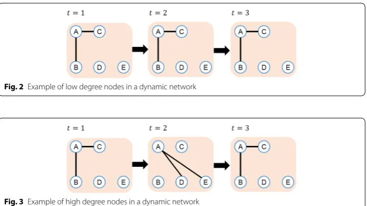
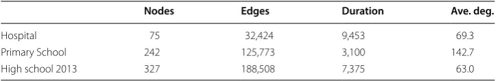
where N(v, t) is a collection of nodes adjacent to node v at time t. Figures 2 and 3 illus-trate the examples of degrees on dynamic networks. In Fig. 2, adjacent nodes of node
A do not change during the period. The difference of adjacent nodes N(A, 1)\N(A, 2) and N(A, 2)\N(A, 3) is empty. Therefore, the degree of node A in Fig. 2 is calculated as follows.
On the other hand, in Fig. 3, nodes adjacent to node A change over time. So the degree of node A is bigger than that in Fig. 2.
In Figs. 2 and 3, the number of adjacent nodes of node A is the same every time, so the average degree of node A is the same in Figs. 2 and 3. On the other hand, if we employ DT(v) as the definition of node degree, D3(A)=0 in Fig. 2, and D3(A)=2 in Fig. 3.
DT(v) captures the number of newly adjacent nodes, and this is important for influence maximization problem. We therefore employ DT(v) as the definition of node degree in dynamic networks.
D3(A)= |N(A, 1)\N(A, 2)|
|N(A, 1)∪N(A, 2)||N(A, 2)| +
|N(A, 2)\N(A, 3)|
|N(A, 2)∪N(A, 3)||N(A, 3)|
=0
2×2+ 0
2 ×2=0
D3(A)=
|N(A, 1)\N(A, 2)|
|N(A, 1)∪N(A, 2)||N(A, 2)| +
|N(A, 2)\N(A, 3)|
|N(A, 2)∪N(A, 3)||N(A, 3)|
=2
4 ∗2+ 2 4∗2=2
Fig. 2 Example of low degree nodes in a dynamic network
Influence maximization methods for dynamic networks
There are two approaches for influence maximization problem in dynamic networks: methods based on Monte-Carlo simulation and heuristic-based methods. The former
method is proposed by Habiba and Berger-Wolf [2]. The method estimates the scale of
propagation σ (·) by repeating Monte-Carlo simulation just the same as in static
net-works. Since σ (·) is monotonic and deteriorated modular also in dynamic networks,
this method achieves large-scale propagation. However, the computational cost of this
method is high as in static networks. Osawa and Murata [25] proposed a heuristic
method for calculating σ (·) at high speed. His algorithm for computing σ (S) for seed nodes S is shown as follows.
calculated approximately, and it is worse compared with the solutions by Monte-Carlo simulation.
Proposed methods
We propose new methods for influence maximization problem in dynamic networks in this section. We propose three new methods (Dynamic Degree Discount, Dynamic CI, and Dynamic RIS) which are the extensions of static network methods to dynamic net-work methods. We use the following notations: G: dynamic network, T: duration of the dynamic network, k: the size of seed nodes, : susceptibility, θ : the number of generated networks, and S: seed nodes.
Dynamic Degree Discount
Dynamic Degree Discount is the extension of Degree Discount by Chen et al. [17] to
Dynamic CI
Dynamic CI is an extension of Morone’s method [18] for dynamic networks. Morone’s
method focuses on the degree of node v and the degrees of nodes with distance l from
v. Dynamic CI defines an index D_CIl(v) in which degree and distance are extended to dynamic networks.
The differences between CIl(v) and D_CIl(v) are as follows: (1) the definition of degree is changed to that for dynamic networks and (2) ∂Ball(v,l) in CIl(v) is changed to
DBall(v, l). DBall(v, l) represents nodes where their shortest duration of time (men-tioned in “Model of information propagation” section) from node v is l. l is a param-eter which takes the value within the range 1≤l≤T . In the algorithm of Dynamic CI,
D_CIl(v) is computed for each node and top k nodes are selected as seed nodes.
Dynamic RIS
Dynamic RIS is an extension of Borgs’s method [20] and Tang’s method [21] for dynamic networks.
The difference between Borgs’s and Tang’s algorithm and Dynamic RIS is where RR in their algorithm is set as RR(v, d) in our algorithm. RR(v, d) is a set of all nodes that are reachable to v within the shortest duration of time d in all durations of dynamic net-works, which is defined as follows:
D_CIl(v)=DT(v)
RRt(v,d) is a set of nodes which are reachable to “node v at time t” within the shortest period of d.
The computational complexities of these methods are as follows.
Dynamic Degree Discount
According to the paper of Chen et al. [17], the computational complexity of Degree Dis-count is O(k·logn+m) , where k is the number of seed nodes, n is the number of nodes, and m is the number of edges, respectively. Dynamic Degree Discount is an extension of Degree Discount. Static degree is replaced with dynamic one ( DT(i) ) and Static
neigh-bors is replaced with dynamic one ( NT(v) ). Computational complexity for dynamic
degree and dynamic neighbors is T·m
n , where T is the total duration of time of given dynamic network. Therefore, the total computational complexity of Dynamic Degree Discount is O(k·logn+m+ Tn·m).
Dynamic CI
According to the paper of Morone and Makse [18], the computational complexity of
CI is O(n·logn) , where n is the number of nodes. Dynamic CI is an extension of CI. Static degree is replaced with dynamic one ( DT(i) ), and its computational complexity is
T·m
n , where T is the total duration of time of given dynamic network. Therefore, the total computational complexity of Dynamic CI is O(n·logn+ Tn·m).
Dynamic RIS
According to the paper of Tang et al. [21], the computational complexity of RIS is
O(k·l2(m+n)log2n/ǫ3) which returns (1−1e−ǫ)-approximate solution with at least
1−n−l probability, where l and ǫ are the constants. Computational complexity of Dynamic RIS heavily depends on the parameters θ and d, which are the number of gen-erated networks and the duration of time for computing RR(v, d), respectively. Therefore, the total computational complexity of Dynamic RIS is O(θ·d·k·l2(m+n)log2n/ǫ3).
Experiments
We perform experiments for comparing the proposed methods with previous ones in order to confirm their effectiveness. Dynamic networks used for the experiments are shown in Table 1. These networks are the same as the ones used in previous research.
Average degree in Table 1 shows the average of all nodes in the network, which is
1 |V|
v∈V DT(v) . Hospital [27] is a network about contacts of patients and medical staffs at hospital with time. Primary School [28, 29] is a network about contacts of students and teachers at school. High School 2013 [30] is a network of contacts of students. The unit of the duration in these three datasets is 20 s. Each dataset is available at SocioPat-terns (http://www.socio patte rns.org).
RR(v,d)= T
t=1
Methods used in the experiments are previous two methods (Monte-Carlo simulation
(MC Greedy) and Osawa) for dynamic network explained in “Influence maximization
methods for dynamic networks” section and our proposed methods (Dynamic Degree
Discount, Dynamic CI, and Dynamic RIS) in “Proposed methods” section. Given a
net-work as input, each method computes seed nodes S. The simulation of influence
maxi-mization based on SI model is repeated R times with the obtained seed nodes and set
the average of the number of nodes in state I as σ (S) . The values of σ (S) are compared in order to evaluate the methods.
Experiments are performed for the following purposes:
(1) Comparison of σ (S) when the size of seed nodes k changes.
(2) Comparison of computational time when the size of seed nodes k changes.
Parameters in the experiments are set as follows. The number of repetition of the simulations for information propagation is set as R=50 . The number of repetition of Monte-Carlo simulation in MC Greedy is set as 1000. These two parameters are com-mon in all experiments. The size of seed nodes k is set from 0 to 20%. Susceptibility is set as =0.01 . It is difficult to perform experiments for all the values as parameter l in Dynamic CI which takes the value of 1≤l≤T . We use the values l=1, 5, 10, 20 in the experiments. As the parameters θ and d in Dynamic RIS, θ is set as θ =1000 and as for
d, values d=0, 5, 10, 20 are used since it is difficult to perform experiments for all the
value as in l of Dynamic CI.
CELF [31] is used to speedup the experiments when greedy algorithms are used in MC Greedy and Osawa. CELF is an algorithm used when the greedy algorithm is applied to the problem with inferior modularity, and the solution is the same as in normal greedy
algorithm. According to the experiments by Lescovec [31], computational time is 700
times faster than normal greedy algorithm when CELF is used.
Experimental results
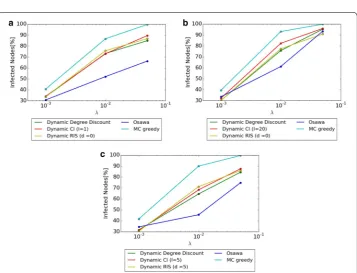
Comparison of σ (S) when the size of seed nodes k changes
The results of information propagation for each size of seed nodes k with fixed suscepti-ble =0.01 of SI model are shown in Fig. 4. The x axis of the Figure shows the percent-age of seed nodes, and the y axis shows the number of infected nodes. Values of the x
axis is k
|V|×100 , the percentage of seed nodes to all nodes in the network. Values of the
y axis is σ (S)
|V| ×100 , the percentage of σ (S) to all nodes in the network. The best values of
l in Dynamic CI and d in Dynamic RIS are used in our experiments. As shown in Fig. 4, MC Greedy achieves the highest diffusion in all datasets. Diffusion of the proposed
Table 1 Dataset for the experiments
Nodes Edges Duration Ave. deg.
Hospital 75 32,424 9,453 69.3
Primary School 242 125,773 3,100 142.7
Fig. 4 Comparison of σ (S) when the size of seed nodes k changes. a Hospital. b Primary School. c High School 2013
methods, Dynamic Degree Discount, Dynamic CI, and Dynamic RIS are inferior to MC Greedy, but they are still better than Osawa. The scale of diffusion of Dynamic RIS in High School 2013 achieves 1.5 times as in Osawa.
There is not much difference in the scale of diffusion among each of the three pro-posed methods. Dynamic RIS achieves the highest in High School 2013, for example, but the difference among proposed methods is small compared with the difference between proposed methods and previous methods (MC Greedy and Osawa).
Comparison of σ (S) when susceptibility changes
Figure 5 shows diffusion when the size of seed nodes is fixed as 20% of all nodes in the networks and susceptibility is changed as =0.001, 0.01, 0.05 . The x axis shows the value of , and the y axis shows the percentage of diffusion. Parameters l and d are the
same as the ones used in the previous experiments. As shown in Fig. 5, MC Greedy
achieves the highest diffusion regardless of the value of . The difference among three proposed methods is small.
As the result of comparison with proposed methods and Osawa, our proposed methods achieve higher scale of diffusion than Osawa in Hospital and High School
2013 when =0.05 . Osawa achieves higher diffusion than Dynamic RIS only in
Pri-mary School. When =0.001 , the difference between proposed methods and Osawa
is very small compared with the cases of other values.
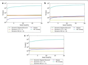
Comparison of computational time when the size of seed nodes k changes
Figure 6 shows the computational time when is set as =0.01 and the sizes of seed nodes are changed. A PC of Intel Core i7(3.4 GHz) CPU and 8 GB memory is used for the experiments. X axis shows the percentage of seed nodes, and y axis shows the computational time (log-scale).
Figure 6 shows that for all datasets, methods other than MC Greedy can compute
seed nodes in realistic time. MC Greedy needs several hours to compute seed nodes. This shows that MC Greedy is intractable in realistic time for large-scale networks.
Regarding the comparison among three proposed algorithm, computational time of Dynamic Degree Discount and Dynamic CI is almost the same in all datasets. Dynamic RIS is about the same computational time as the other two proposed meth-ods in Hospital, and is faster in Primary School and High School 2013. Regarding the
comparison with proposed methods and Osawa, Dynamic RIS is approximately 7.8 times faster than Osawa except very small network (Hospital).
Parameters of Dynamic CI and Dynamic RIS
Diffusions of proposed methods with different parameters are shown in this section. We change parameters l of Dynamic CI, and θ and d in Dynamic RIS.
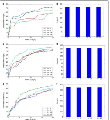
Diffusion and computational time of different l in Dynamic CI
Diffusion and computational time when l in Dynamic CI changes to 1, 5, 10, 20 are
shown in Fig. 7. Left line graphs show the size of diffusion when l is changed in each network. Right bar graphs show computational time. Left line graphs show that diffusion depends on the value of l. Therefore, it is important to find appropriate l in Dynamic
CI. Since there is no simple correlation between the scale of diffusion and the value of
l (such as diffusion becomes larger as l becomes large), diffusions for various values of l
should be investigated and compared. Right bar graphs show that there are no big differ-ences of execution time when the value of l changes.
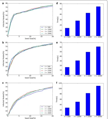
Diffusion and computational time of different θ in Dynamic RIS
θ in Dynamic RIS is a parameter for the number of generated graphs in RR(v, d).
Dif-fusion and computational time when parameter θ is changed to 500, 1000, 1500, 2000
are shown in Fig. 8. Left line graphs show that diffusion does not change much when
θ changes. However, the scale of diffusion is slightly small when θ =500 in Hospital
and High School 2013. This means that bigger θ is desirable from the viewpoint of
diffusion. On the contrary, right bar graphs show that higher value of θ results in the
increase of computational time. From the viewpoint of computational time, smaller θ
is better. Regarding the value of θ , there is a trade-off between the scale of diffusion
and the computational time. It is important to find smaller θ for shorter
computa-tional time, but too small θ results in small-scale diffusion.
Diffusion and computational time of different d in Dynamic RIS
d in Dynamic RIS is a parameter for the number of time steps for looking back.
Fig-ure 9 shows diffusion and executing time when parameter d changes to 0, 5, 10, 20. Left line graphs show that there is almost no difference in diffusion when d changes, while right bar graphs show that computational time increases as the value of d becomes big-ger. The scale of diffusion does not change even if the value of d becomes bigger in our experiments.
Discussion
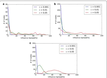
Analysis focused on expansion of each node
In the experiments when susceptibility changes in “Advantages and disadvantages of
each of the proposed methods” section, the difference between the proposed methods
and Osawa was small when =0.001 compared with the experiments with other
val-ues of . When =0.05 , Osawa outperforms proposed methods only in Primary School. This section discusses these two points.
Figure 10 shows the distribution of diffusion σ ({v}) of each node v when Monte-Carlo simulation is used. X axis shows the percentage of diffusion from node v to the whole network ( σ ({v}) ), and Y axis shows the frequency of the nodes with each of the percentage in X axis. When =0.001 , almost all nodes are less than 5% of diffusion in
all networks. This means that there is no big difference of the diffusion from different seed nodes. This is the reason why the difference between proposed methods and Osawa
is small in the experiment in “Advantages and disadvantages of each of the proposed
methods” section. On the contrary, there are many nodes with more than 60% of
diffu-sion in Primary School when =0.05 compared with other two networks. In this case,
large-scale diffusion is easy to be achieved even if the most appropriate seed nodes are not selected. This is the reason why Osawa outperforms proposed method in Primary School in “Advantages and disadvantages of each of the proposed methods” section.
Advantages and disadvantages of each of the proposed methods
Advantages and disadvantages of each of the proposed methods are discussed in this section. An advantage of Dynamic Degree Discount is that it contains no parameter, so there is no need to adjust parameter. Its disadvantage is that it is only for SI model, so the method cannot be used for other models. This is because Dynamic Degree Discount is an extension of Chen’s Degree Discount which is for SI model. There are other informa-tion propagainforma-tion models such as LT model and Triggering models proposed by Kempe et al. Dynamic Degree Discount cannot be applied to such models.
An advantage of Dynamic CI is that it can be applied to many information propaga-tion models in contrast to Dynamic Degree Discount because Dynamic CI uses only degree information when it calculates seed nodes. Its disadvantage is that the
abil-ity of diffusion depends on the value of parameter l as mentioned in “Diffusion and
computational time of different l in Dynamic CI” section. It is necessary to search for
appropriate values of l for Dynamic CI. The parameter l takes the value within the
range 1<l<T , so the search takes time in general.
An advantage of Dynamic RIS is that its computational time is short. As shown in the experimental results, its computational time is shorter than other methods in all networks except Hospital. As the method can be applied to large networks due to its short computational time, this is a big advantage. Disadvantage of Dynamic RIS is that it needs to adjust parameters θ and d. As mentioned in the previous section,
computational time becomes bigger as the parameter θ becomes bigger, and the scale
of diffusion becomes smaller for too small θ . Therefore, it is necessary to set appropri-ate value for θ . However, parameter sensitivity of θ and d is not so much compared with the sensitivity of l in Dynamic CI.
Conclusion
Osawa, the performances of these three methods are almost the same as Osawa, but they are approximately 7.8 times faster than Osawa. Based on these facts, the pro-posed methods are suitable for influence maximization in dynamic networks.
The comparison of Dynamic Degree Discount, Dynamic CI, and Dynamic RIS is as follows. The choice of the methods should be done based on the following pros and cons.
Dynamic Degree Discount
• It requires no parameter. • It is applicable to SI model only.
Dynamic CI
• It is applicable to other information propagation models. • The performance heavily depends on parameter l.
Dynamic RIS
• It is relatively fast among these three methods. • It requires two parameters to be adjusted ( θ and d).
Finding the strategies of choosing suitable method for given dynamic network is practi-cally important. It is a challenging open question and is left for our future work.
The problem of adjusting the parameters for Dynamic CI and Dynamic RIS is also left for our future work.
Authors’ contributions
The authors propose three new methods for influence maximization problem in dynamic networks. Both authors read and approved the final manuscript.
Acknowledgements
The authors would like to thank the funding partners for supporting our work. Competing interests
The authors declare that they have no competing interests. Availability of data and materials
Data are available at SocioPatterns (http://www.socio patte rns.org). Funding
This work was supported by JSPS Grant-in-Aid for Scientific Research(B) (Grant Number 17H01785) and JST CREST (Grant Number JPMJCR1687).
Publisher’s Note
Springer Nature remains neutral with regard to jurisdictional claims in published maps and institutional affiliations.
Received: 20 February 2018 Accepted: 15 September 2018
References
1. Kempe D, Kleinberg J, Tardos É. Maximizing the spread of influence through a social network. In: Proceedings of the Ninth ACM SIGKDD international conference on knowledge discovery and data mining-KDD ’03. p. 137–46. 2003.
https ://doi.org/10.1145/95675 0.95676 9.
3. Murata T, Koga H. Methods for influence maximization in dynamic networks. In: Proceedings of the 6th international conference on complex networks and their applications (Complex Networks 2017), studies in computational intel-ligence. Berlin: Springer; 2017. p. 955–66.
4. Babaei M, Mirzasoleiman B, Jalili M, Safari MA. Revenue maximization in social networks through discounting. Soc Netw Anal Mining. 2013;3(4):1249–62.
5. Jalili M. Social power and opinion formation in complex network. Phys A. 2013;392(4):959–66. 6. Jalili M. Effects of leaders and social power on opinion formation in complex networks. Simulation.
2012;89(5):578–88.
7. Afshar M, Asadpour M. Opinion formation by informed agents. J Artif Soc Soc Simul. 2010;13(4):1–5. 8. Garimella K, Morales GDF, Mathioudakis M, Gionis A. Polarization on social media. Web Conf 2018 Tutorial.
2018;1(1):1–191.
9. Braha D, Bar-Yam Y. From centrality to temporary fame: dynamic centrality in complex networks. Complexity. 2006;12(2):59–63.
10. Braha D, Bar-Yam Y. Time-dependent complex networks: Dynamic centrality, dynamic motifs, and cycles of social interactions. In: Adaptive networks: theory, models and applications. 2009. p. 39–50.
11. Hill SA, Braha D. Dynamic model of time-dependent complex networks. Phys Rev E. 2010;82(046105):1–7. 12. Holme P. Modern temporal network theory: a colloquium. Eur Phys J B. 2015;88(234):1–30.
13. Holme P, Saramäki J. Temporal networks. Phys Rep. 2012;519(3):97–125. https ://doi.org/10.1016/j.physr ep.2012.03.001.1108.1780.
14. Jalili M, Perc M. Information dascades in complex networks. J Compl Netw. 2017;5(5):665–93.
15. Chen W, Wang C, Wang Y. Scalable influence maximization for prevalent viral marketing in large-scale social net-works. In: Proceedings of the 16th ACM SIGKDD international conference on knowledge discovery and data mining-KDD ’10. 2010. p. 1029–38. https ://doi.org/10.1145/18358 04.18359 34.
16. Jiang Q, Song G, Cong G, Wang Y, Si W, Xie K. Simulated annealing based influence maximization in social networks. In: Proceedings of the twenty-fifth AAAI conference on artificial intelligence. 2011. p. 127–132.
17. Chen W, Wang Y, Yang S. Efficient influence maximization in social networks. In: Proceedings of the 15th ACM SIGKDD international conference on knowledge discovery and data mining-KDD ’09. 2009. p. 199–207. https ://doi. org/10.1145/15570 19.15570 47.1204.4491. http://porta l.acm.org/citat ion.cfm?doid=15570 19.15570 47.
18. Morone F, Makse HA. Influence maximization in complex networks through optimal percolation. Nature. 2015;524(7563):65–8. https ://doi.org/10.1038/natur e1460 4.
19. Ohsaka N, Akiba T, Yoshida Y, Kawarabayashi K-i. Fast and accurate influence maximization on large networks with Pruned Monte-Carlo simulations. In: Proceedings of the twenty-eighth AAAI conference on artificial intelligence. 2014. p. 138–44.
20. Borgs C, Brautbar M, Chayes J, Lucier B. Maximizing social influence in nearly optimal time. In: Proceedings of the twenty-fifth annual ACM-SIAM symposium on discrete algorithms. 2014. p. 946–57.
21. Tang Y, Xiao X, Shi Y. Influence maximization: near-optimal time complexity meets practical efficiency. In: Proceed-ings of the 2014 ACM SIGMOD international conference on management of data. 2014. p. 75–86.
22. Chen W, Lu W, Zhang N. Time-critical influence maximization in social networks with time-delayed diffusion process. In: Proceedings of the twenty-sixth AAAI conference on artificial intelligence. 2012. p. 592–8. http://www.aaai.org/ ocs/index .php/AAAI/AAAI1 2/paper /viewF ile/5024/5243http://arxiv .org/abs/1204.3074.
23. Feng S, Chen X, Cong G, Yifeng Z, Yeow, Meng C, Yanping X. Influence maximization with novelty decay in social networks. In: Proceedings of the twenty-eighth AAAI conference on artificial intelligence. 2014. p. 37–43.
24. Mihara S, Tsugawa S, Ohsaki H. Influence maximization problem for unknown social networks. In: Proceedings of the 2015 IEEE/ACM international conference on advances in social networks analysis and mining 2015-ASONAM ’15. 2015. p. 1539–46. https ://doi.org/10.1145/28087 97.28088 85.
25. Osawa S, Murata T. Selecting seed nodes for influence maximization in dynamic networks. In: Proceedings of the 6th workshop on complex networks (CompleNet 2015), studies in computational intelligence. Berlin: Springer; 2015. p. 91–8.
26. Habiba, Yu Y, Berger-Wolf TY, Saia J. Finding spread blockers in dynamic networks. In: Advances in social network mining and analysis. 2010. vol. 5498, p. 55–76.
27. Vanhems P, Barrat A, Cattuto C, Pinton J-F, Khanafer N, Régis C, Kim B-A, Comte B, Voirin N. Estimating potential infec-tion transmission routes in hospital wards using wearable proximity sensors. PloS ONE. 2013;8(9):73970.
28. Stehle J, Voirin N, Barrat A, Cattuto C, Isella L, Pinton JF, Quaggiotto M, Van den Broeck W, Regis C, Lina B, Vanhems P. High-resolution measurements of face-to-face contact patterns in a primary school. PloS ONE. 2011;6(8):23176. 29. Gemmetto V, Barrat A, Cattuto C. Mitigation of infectious disease at school: targeted class closure vs school closure.
BMC Infect Dis. 2014;14(1):1.
30. Mastrandrea R, Fournet J, Barrat A. Contact patterns in a high school: a comparison between data collected using wearable sensors, contact diaries and friendship surveys. PloS ONE. 2015;10(9):0136497.