O R I G I N A L R E S E A R C H
Open Access
Fourth-order stable central difference with
Richardson extrapolation method for
second-order self-adjoint singularly
perturbed boundary value problems
Muslima Kedir Siraj, Gemechis File Duressa and Tesfaye Aga Bullo
** Correspondence:tesfayeaga2@ gmail.com
Fourth-order stable central difference with Richardson extrapolation method has been formulated for solving second-order self-adjoint singularly perturbed boundary value problems using the study design of both documentary review and numerical experimental using MATLAB R2013a software which gives more accurate numerical solution with the corresponding sixth-order convergent.
Department of Mathematics, Jimma University, P. O. Box 378, Jimma, Ethiopia
Abstract
This study introduces a stable central difference method for solving second-order self-adjoint singularly perturbed boundary value problems. First, the solution domain is discretized. Then, the derivatives in the given boundary value problem are replaced by finite difference approximations and the numerical scheme that provides algebraic systems of equations is developed. The obtained system of algebraic equations is solved by Thomas algorithm. The consistency and stability that guarantee the convergence of the scheme are investigated. The established convergence of the scheme is further accelerated by applying the Richardson extrapolation which yields sixth order convergent. To validate the applicability of the method, two model examples are solved for different values of perturbation parameterεand different mesh sizeh. The proposed method approximates the exact solution very well. Moreover, the present method is convergent and gives more accurate results than some existing numerical methods reported in the literature.
Keywords:Singular perturbation, self-adjoint problem, boundary value problem,
finite difference method, Richardson extrapolation
Mathematics subject classification:65L10, 65L11, 65L12, 65B05, 65Y04
Introduction
Any differential equation obtained from a given differential equation and having the property that its solution is an integrating factor of the other is known as adjoint dif-ferential equation. Self-adjoint singularly perturbed difdif-ferential equation is a difdif-ferential equation whose highest order derivative is multiplied by a small positive parameter and that has the same solution as its adjoint equation [1, 2]. In a singularly perturbed problem, small positive parameter affects the highest order derivative(s) of the differen-tial equation which gives rise to large gradients in the solution over narrow regions of the domain, so that the presence of a small perturbation parameter in the differential equation typically leads to boundary layers in the solution, which makes the conver-gence analysis very difficult [3]. As Miller et al. [2], boundary layer is a region of the in-dependent variable over which the in-dependent variable changes rapidly.
Singularly perturbed second-order boundary value problem occur very frequently in fluid motion, chemical reactor theory, elasticity, diffusion in polymer, reaction-diffusion
equation, control of chaotic system, and so on [4]. Upon settingε= 0, if the order of
singularly perturbed differential equations is reduced by one, then the problem is called convection-diffusion type and if the order is reduced by two, it is called reaction-diffusion type. Hence, second-order singularly perturbed self-adjoint ordinary differen-tial equations are types of reaction-diffusion problems. Since the solution of this problem exhibits one or two layers, the existing numerical methods give good results
only when the mesh size his smaller than the perturbation parameterε(i.e.,h≤ε). But
it is an expensive and time-consuming process. If we take h≥ε, the existing classical
numerical methods produce oscillatory solution and pollute the solution in the entire interval, because of boundary layer behavior. In connection to this, there are some numerical methods suggested by various authors for solving self-adjoint singular per-turbation problems, namely, initial value technique [5], quintic spline method [6], non-polynomial spline functions method [7], difference scheme using cubic spline [8], finite difference method with variable mesh [9], fitted mesh B-spline collocation method [10],
higher order numerical methods [11].
More recently, Fasika et al. [12–14] and Feyisa and Gemechis [15] have developed a
higher (fourth, sixth, eighth, and tenth) order compact finite difference method to solve singularly perturbed reaction-diffusion problems. These authors developed higher order compact finite difference methods for the constant coefficients of diffusion and reaction terms of the problem. Even though their methods give more accurate numerical solu-tions, it is restricted to treat constant coefficient problem. Also, other scholars, Terefe et al. [16] and Yitbarek et al. [17], have presented fourth- and sixth-order stable central difference method, respectively, for solving self-adjoint singularly perturbed two-point boundary value problem. Therefore, the main objective of this study is to develop a stable and more accurate numerical method that works for solving both constant and variable coefficient second-order self-adjoint singularly perturbed boundary value problems.
In this paper, we planned a fourth-order stable central difference with Richardson extrapolation method for solving second-order self-adjoint singularly perturbed bound-ary value problems. First, the derivative in the given differential equation is replaced by the finite difference approximations. Then, the ordinary differential equation converts to a linear system of algebraic equations, and these algebraic equations are transformed to a tri-diagonal system, which can easily be solved by the Thomas algorithm. Further, coding of the program in MATLAB software for the obtained tri-diagonal system has been performed. To validate the applicability of the method, some model examples are considered for numerical experimentation. Both the theoretical and numerical rates of convergence of the scheme have been investigated.
Formulation of the method
Consider the singularly perturbed self-adjoint boundary value problem of the form:
−εa xð Þy0ð Þx 0þb xð Þy xð Þ ¼g xð Þ; x∈Ω≔ð0;1Þ ð1Þ
yð Þ ¼0 α
and
yð Þ ¼1 β ð2Þ
where ε is a perturbation parameter that satisfies 0 <ε< < 1, α, βare given constants and the functions a(x)≠0, b(x)≠0 and g(x) are assumed to be sufficiently continuous differentiable functions. By product rule differentiation, Eq. (1) can be re-written as:
−εy″ð Þ þx p xð Þy0 x
ð Þ þq xð Þy xð Þ ¼f xð Þ ð3Þ
where
p xð Þ ¼−εa
0 x
ð Þ
a xð Þ ; q xð Þ ¼
b xð Þ
a xð Þ
and
f xð Þ ¼a xg xð Þ
ð Þ:
In order to develop the finite difference method, the interval [0, 1] is divided into N
equal sub-intervals with set of grid pointsxi=x0+ih, fori= 0, 1, 2, ...,N, whereh¼N1.
For convenience, letpðxiÞ ¼pi;qðxiÞ ¼qi;yðxiÞ ¼yi;y 0
ðxiÞ ¼y0i; :::;yðnÞðxiÞ ¼yðinÞ:
Assume that y(x) has continuous higher order derivatives on [0, 1], and to develop
the fourth-order stable central difference scheme, we use Taylor’s series expansion in order to get central difference formula foryi′′andyi′.
yiþ1¼yiþhyi0þh2!2yi00þh3
3!yi 000
þh4!4yð Þ4
i þ
h5 5!y
5
ð Þ
i þ
h6 6!y
6
ð Þ
i þ::: ð4Þ
yi1¼yi−hyi0þh2!2yi00−h3
3!yi 000
þh4!4yð Þ4
i −
h5 5!y
5
ð Þ
i þ
h6 6!y
6
ð Þ
i þ::: ð5Þ
From Eqs. (4) and (5), we have:
yi0 ¼yiþ1−yi−1 2h −
h2 6 y
‴
i − h4 120y
5
ð Þ
i þτ1 and yi 00
¼yiþ1−2yiþyi−1
h2 −
h2 12y
4
ð Þ
i þτ2 ð6Þ
whereτ1¼−h
6
7! yið7Þandτ2¼−h
4
360yið6Þ
Substituting Eq. (6) into the discrete form of Eq. (3) gives:
qiyiþ2phi yiþ1−yi−1
−ε
h2 yiþ1−2yiþyi−1
−pih2 6 y
‴ i þεh
2
12y
4
ð Þ
i −pih
4
120y
5
ð Þ
i þτ0¼fi ð7Þ
where
τ0¼piτ1−ετ2
Differentiating Eq. (3) successively and considering at the nodal points yields:
yi000
¼1ε piyi00þ p
i 0
þqi
yi0þqi0yi−fi0
ð8Þ
yið Þ4 ¼1
ε piyi 000
þ 2pi0þqi
yi00
þ pi00
þ2qi0
y0
iþqi00yi−fi 00
yið Þ5 ¼1
ε piyið Þ4 þ 3p 0 iþqi
y‴
i þ 3pi 00
þ3qi0
yi00þ p‴
i þ3q″
y0iþqi‴y
i−f‴i
ð10Þ
Using Eq. (10), the term which containsyi(5)from Eq. (7) becomes:
−pih4 120 yi
5
ð Þ¼−pi2h4
120εyi 4
ð Þ−pihð Þ4
120ε 3pi
0
þqi
yi000 −pihð Þ4
120ε 3p ″
i þ3q 0 i
y″
i −pih4
120ε p ‴
i þ3q″i
y0i−piqi000h4
120ε yiþ pih4 120εf
‴
i
ð11Þ
Also, from Eqs. (4) and (5), we have the central finite difference approximation:
yi0 ¼yiþ1−yi−1 2h þτ3
and
yi00
¼yiþ1−2yiþyi−1
h2 þτ4 ð12Þ
where
τ3¼− h2 6 y
‴
i
and
τ4¼− h2 12y
4
ð Þ
i
Putting Eq. ((12), into Eq. (11) gives:
−pih4 120 yi
5
ð Þ¼−pi2h4
120εyi 4
ð Þ−pihð Þ4
120ε 3pi
0
þqi
yi000
− pih2
120ε 3p ″
i þ3q 0 i
yiþ1−2yiþyi−1
− pih3
120ε p ‴
i þ3q″i
yiþ1−yi−1
−piqi000h4
120ε yiþ pih4 120εf
‴
i þτ5
ð13Þ
where
τ5¼− pih4 120ε p
‴
i þ3q″i
τ3− pih4 120ε 3p
″
i þ3q 0
τ4:
Substituting Eq. (13) into Eq. (7) and rearranging, we get:
qi−piq‴i h4
120ε
yiþ pi
2h− pih3 240ε p
‴
i þ3q″i
yiþ1−yi−1
− hε2þ p2
i
120ε 3p ″
i þ3q 0 i
yiþ1−2yiþyi−1
− pih2 6 þ
pih4 120ε 3p
0 iþqi
y‴
þ εh2
12− p2
ih2
120ε
y4
i þτ6¼ fi− pih4 120εf
‴
i
ð14Þ
where
τ6¼τ0þτ5
εh2 12−
p2
ih4
120ε
yi4¼ pih2
12 − p3
ih4
120ε2
y‴
i þ
q″
ih2
12 − p2
iq″ih4
120ε2
yiþτ7
þ 1
12− p2
ih2
120ε2
2p0iþqi
yiþ1−2yiþyi−1
þ h
24− p2
ih3
240ε2
p″
i þ2q 0 i
yiþ1−yi−1
− h2 12−
p2
ih4
120ε2
f″
i
ð15Þ
whereτ7¼ ðh
2
12−
pi2h4
120ε2Þð2p
0
iþqiÞτ4þ ðh
2
12−
pi2h4
120ε2Þðp″i þ2q
0 iÞτ3 Substituting Eq. (15) into Eq. (14) yields:
qi−piq‴i h4
120ε þ q‴
i h2
12 − p2
iq‴i h4
120ε2
yi
þ pi
2h− pih3 240ε p
‴
i þ3q″i
þ h
24− p2
ih3
240ε2
p″
i þ2q 0 i
yiþ1−yi−1
− hε2þ pih2
120ε 3p ″
i þ3q 0 i − 1 12− p2
ih2
120ε2
2p0iþqi
yiþ1−2yiþyi−1
þ pih2
12 þ pih4 120ε 3p
0 iþqi
−pih2
6 þ pi3h4 120ε2
y‴þτ 8
¼ fiþ h2
12þ pi2h4 120ε2
f″
i− pih4 120εf
‴
i
ð16Þ
where
τ8¼τ6þτ7:
For simplicity, let
Ai¼qi−piq
‴
ih4 120ε þ
q‴
ih2 12 −
p2
iq‴ih4 120ε2 ;Bi¼
pi 2h−pih
3
240εðp‴i þ3q″iÞ þ ð24h −
p2
ih3
240ε2Þðp″i þ2q
0 iÞ
Ci¼hε2þpih
2
120ε 3p ″
i þ3q 0 i − 1 12− p2
ih2
120ε2
2p0iþqi
Di¼pih
2
12 −
pih4 120εð3p
0
iþqiÞ−pih
2
6 −
pi3h4
120ε2;HhðiÞ ¼ fiþ ðh 2
12þ
pi2h4 120ε2Þf″i−
pih4 120εf
‴
Then, Eq. (16) re-written as:
AiyiþBi yiþ1−yi−1
−Ci yiþ1−2yiþyi−1
þDiy‴i þτ8¼Hh ið Þ ð17Þ
Lastly, using Eq. (8), the term that containsy‴i from Eq. (17) becomes:
Diyi
000 ¼piDi
ε yiþ1−2yiþyi−1
þ Di 2hε pi
0 þqi
yiþ1−yi−1
þDiqi0
ε yi−Dεifi
0
þτ9 ð18Þ
where
τ9¼ piDi
ε τ4þ Di
ε τ3
Putting Eq. (18) into Eq. (17), and write in three-term recurrence relation:
−Eiyi−1þFiyi−Giyiþ1þτ10¼Hi ð19Þ
whereEi¼Ci−pεihD2iþBiþ Di 2hεðpi
0
þqiÞ; Fi¼AiþDiq
0
i
ε þ2ðCi−PεihD2iÞGi¼Ci− PiDi
εh2−Bi− Di 2hε
ðpi0
Richardson extrapolation
The basic idea behind extrapolation is that whenever the leading term in the error for an approximation formula is known, we can combine two approximations obtained
from the formula using different values of the mesh sizeshand 0.5hto obtain a higher
order approximation and the technique is known as Richardson extrapolation. This procedure is a convergence acceleration technique which consists of a linear combin-ation of two computed approximcombin-ations of a solution (applied on two nested meshes). The linear combination turns out to be a better approximation.
Since the truncation error of the formulated method Eq. (19) isO(h4), we have
jy xð Þi −YNj ≤C h4 ð20Þ
wherey(xi) and YNare exact and approximate solutions respectively, Cis constant
in-dependent of mesh sizesh.
LetΩ2Nbe the mesh obtained by bisecting each mesh interval inΩNand denote the
approximation of the solution on Ω2N by Y2N. Consider Eq. (20) works for any h≠0,
which implies:
y xð Þi −YN≤C h4 þRN; xi∈ΩN ð21Þ
So that it also works for anyh2≠0 and yields:
y xð Þi −Y2N≤C h 2 4!
þR2N; x
i∈Ω2N ð22Þ
where the remainders,RN and R2N, are of O(h6). A combination of inequalities in Eqs. (21) and (22) leads to 15y(xi)−(16Y2N−YN)≈O(h6), which suggests that
YN
ð Þext¼ 1
15ð16Y2N−YNÞ ð23Þ
is also an approximation of y(xi). Using this approximation to evaluate the truncation
error, we obtain:
jy xð Þi −ðYNÞextj ≤Ch6 ð24Þ
Now, using the solutions obtained by the scheme given by Eq. (19), we get another
third solution in terms of the two by Eq. (23). This is Richardson extrapolation method
for the fourth-order finite-difference scheme only to accelerate the rate of convergence to sixth order.
Consistency of the method
Local truncation errors refer to the differences between the original differential equation and its finite difference approximations at grid points. Local truncation errors measure how well a finite difference discretization approximates the differential equation [18]. In our case, the last truncation error in Eq. (19) isτ10=τ8+τ9.
But, from Eqs. (16) and (17), we haveτ8=τ6+τ7andτ9¼piεDiτ4þDεiτ3, So that:
τ10¼τ6þτ7þ piDi
ε τ4þ Di
τ10¼τ0þτ5þτ7þ piDi
ε τ4þ Di
ε τ3;
because of Eq. (13)
Also, from Eqs. (13) and (15), we have:
τ5¼− pih4 120ε p
‴
i þ3q″i
τ3− pih4 120ε 3p
″
i þ3q 0
τ4
τ7¼ h2 12−
pi2h4 120ε2
2p0iþqi
τ4þ h2 12−
pi2h4 120ε2
p″
i þ2q 0 i
τ3
Hence, the truncation errors are re-written as:
τ10¼τ0þ Di
ε þ h2 12−
pi2h4 120ε2
p″
i þ2q 0 i
−pih4
120ε p ‴
i þ3q″i
τ3
þ piDi
ε þ
h2 12−
pi2h4 120ε2
2p0iþqi
−pih4
120ε 3p ″
i þ3q 0
τ4
ð25Þ
Again, from Eqs. (6), (7), and ((12) into Eq. (25) and after rearranging yields:
jTEj ≤Ch4 ð26Þ
whereTE=τ10and
C¼j1 6y
‴ i
pi 12εþ
pih2 120ε2 3p
0
iþqi
þpi3h2 120ε3þ
1 12−
pi2h2 120ε2
p″ i þ2q
0
i
−pih2 120ε p
‴ i þ3q″i
þ 1 12y 4 ð Þ i p 2 i 12εþ
p2
ih2 120ε2 3p
0
iþqi
þpi4h2 120ε3þ
1 12−
pi2h2 120ε2
2p0iþqi
−pih2 120ε 3p
″ i þ3q
0
þ ε
360yi
6
ð Þ−pih2
5040yi
7
ð Þj
Thus, the developed scheme without applying Richardson extrapolation is fourth order accurate or order of convergence isO(h4). As Zhilin et al. [18], a finite difference scheme is called consistent if the limit of truncation error (TE) is equal to zero as the
mesh sizehgoes to zero. Hence, this definition of consistency on the proposed method
which is given in Eq. (19) with the local truncation error in Eqs. (24) and (26) satisfied as:
lim
h→0TE¼ hlim→0Ch 4¼ lim
h→0 Ch 6¼0
Thus, the proposed method is consistent.
Stability of the method
Consider the developed scheme in Eq. (19) which is given by:
−Eiyi−1þFiyi−Giyiþ1¼Hi
But, the coefficients Ei, Fi and Gi are given in terms of Ai, Bi, Ci and Di with its
values stated in Eq. (17). If we multiply both sides of Eq. (17) by h2and consider the
limit ash→0, we get:
Ai¼Bi¼Di¼0 andCi¼ε ð27Þ
Ei¼Gi¼ε and Fi¼2ε ð28Þ
Considering both Eqs. (27) and (28), into Eq. (19), which can be written in matrix
form:
MY ¼H ð29Þ
where the matrices:
M¼
2ε −ε 0 ⋯ ⋯ 0
−ε 2ε −ε 0 ⋮ ⋮
0 −ε 2ε ⋱ 0 0
0 0 ⋱ ⋱ −ε 0
⋮ ⋮ 0 −ε 2ε −ε
0 ⋯ 0 0 −ε 2ε
2 6 6 6 6 6 6 4
3 7 7 7 7 7 7 5
,Y ¼
y1 y2
⋮ ⋮
yN−2 yN−1 2 6 6 6 6 6 6 4
3 7 7 7 7 7 7 5
and H¼
h2H 1þεy0 h2H
2
⋮ ⋮
h2H
N−2 h2H
N−1þεyN
2 6 6 6 6 6 6 4
3 7 7 7 7 7 7 5
Here,M is a tri-diagonal matrix.Mis irreducible if its co-diagonals contain non-zero
elements only. The co-diagonal contains Ei, Gi. It is easily seen that, for sufficiently
smallh(i.e.h→0),Ei≠0 and Gi≠0,∀i= 1, 2,⋯,N−1.
Hence, M is irreducible. Again, one can observe that∣Ei∣> 0 and∣Gi∣ > 0 and in
each row of M, the sum of the two off-diagonal elements is less than or equal to the
modulus of the diagonal element (i.e.,∣Fi∣ ≥ ∣Ei∣+∣Gi∣). This proves the diagonal
dominance of M. Under these conditions, the Thomas algorithm is stable for
suffi-ciently smallh, as shown in [19].
As proved by Smith [20], the eigenvalues of a tri-diagonal matrix (N−1) × (N−1) of
matrixMare:
λs¼ Fi−2
ffiffiffiffiffiffiffiffiffi EiGi
p
cossπ
N ¼2ε 1−cos sπ N
; s¼1;2;…;N−1 ð30Þ
Also, from trigonometric identity, we have 1−cossπN¼2 sin22sπN. Hence, the
eigen-values of matrixMcan be re-written as:
λs¼2ε 2 sin2 sπ 2N
¼4εsin2 sπ
2N ≤4ε ð31Þ
A finite difference method for the BVPs isstableifMis invertible and
‖M−1‖≤C; ∀0<h<h
0 ð32Þ
whereCandh0are two constants that are independent ofh,[20].
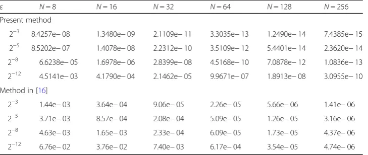
Table 1Comparison of maximum absolute errors for Example 1
ε N= 8 N= 16 N= 32 N= 64 N= 128 N= 256
Present method
2−3 8.4257e−08 1.3480e−09 2.1109e−11 3.3035e−13 1.2490e−14 7.4385e−15
2−5 8.5202e−07 1.4078e−08 2.2312e−10 3.5109e−12 5.4401e−14 2.3620e−14
2−8 6.6238e−05 1.6978e−06 2.8399e−08 4.5168e−10 7.0878e−12 1.0836e−13
2−12 4.5141e−03 4.1790e−04 2.1462e−05 9.9671e−07 1.8913e−08 3.0955e−10
Method in [16]
2−3 1.44e−03 3.64e−04 9.06e−05 2.26e−05 5.66e−06 1.41e−06
2−5 3.71e−03 8.57e−04 2.08e−04 5.09e−05 1.26e−05 3.16e−06
2−8 4.63e−03 1.65e−03 2.33e−04 6.09e−05 1.73e−05 4.37e−06
Since, matrixMis symmetric also its inverse matrixM−1is symmetric and the eigen-valuesM−1is given by 1
λs, we have ‖M−1‖¼ 1
λs¼ 1
4ε≤C;whereCis independent ofh. Thus, the developed scheme in Eq. (19) isstable.
A consistent and stable finite difference method is convergent by Lax’s equivalence
theorem [20]. Hence, as we have shown above, the proposed method is satisfying the
0 0.1 0.2 0.3 0.4 0.5 0.6 0.7 0.8 0.9 1
0 0.1 0.2 0.3 0.4 0.5 0.6 0.7 0.8 0.9 1
x
So
lu
ti
o
n
s
Exact Solution Numerical Solution
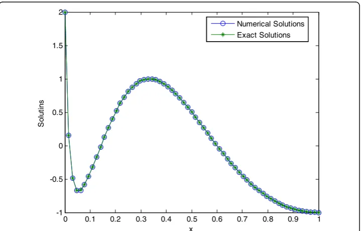
Fig. 1The behavior of exact and numerical solution for Example 1 atε= 10−3andN= 100
0 0.1 0.2 0.3 0.4 0.5 0.6 0.7 0.8 0.9 1
-1 -0.5 0 0.5 1 1.5 2
x
So
lu
ti
n
s
Numerical Solutions Exact Solutions
criteria for both consistency and stability which are equivalents to convergence of the method.
Numerical examples and results
In order to test the validity of the proposed method and to demonstrate their conver-gence computationally, we have taken two model examples of singularly perturbed
self-0 0.1 0.2 0.3 0.4 0.5 0.6 0.7 0.8 0.9 1
0 0.5 1 1.5 2 2.5 3 3.5 4 4.5
5x 10
-3
x
Er
ro
rs
N = 8 N = 16 N = 32
Fig. 3Point-wise absolute errors of Example 1 atε= 2−12with different mesh sizeh
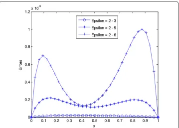
0 0.1 0.2 0.3 0.4 0.5 0.6 0.7 0.8 0.9 1
0 0.2 0.4 0.6 0.8 1 1.2x 10
-9
x
Er
ro
rs
Epsilon = 2 - 3
Epsilon = 2 - 5
Epsilon = 2 - 6
adjoint second-order two-point boundary value problems with exact solutions. The
maximum absolute errors (AE) at the nodal points are given byjAEj¼ max
1≤i≤N−1jyðxiÞ−
ðYNÞextj. And the rate of convergence (R) can be calculated by the formula:
R¼ logðYNÞext−logðY2NÞext
log2
where y(xi) and (YN)ext are exact solution and numerical solution, respectively, at the
nodal pointxi. And for the rate of convergenceYNandY2Nare the numerical solutions obtained on the mesh sizehandh2, respectively.
Example 1:Consider the singularly perturbed self-adjoint problem:
−ε 1þx2y0ð Þx
0
þ1þx−x2y xð Þ ¼f xð Þ; 0<x<1
subject to the boundary conditions y(0) =y(1) = 0, wheref (x) is chosen such that the exact solution is given by:yðxÞ ¼1þ ðx−1Þep−xffiε−xeð1−
xÞ
ffi ε
p
Example 2:Consider the following self-adjoint singular perturbation problem:
−εy″ð Þ þx 4
xþ1
ð Þ4 ðxþ1Þ
ffiffi
ε
p
y xð Þ ¼f xð Þ; 0<x<1
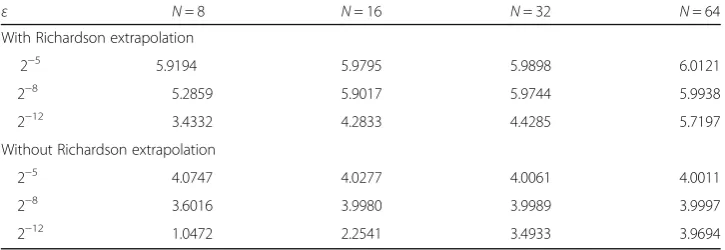
Table 2Comparison between with and without Richardson methods of maximum absolute errors
for Example 1
ε N= 8 N= 16 N= 32 N= 64 N= 128 N= 256
With Richardson extrapolation
2−3 8.4257e−08 1.3480e−09 2.1109e−11 3.3035e−13 1.2490e−14 7.4385e−15
2−5 8.5202e−07 1.4078e−08 2.2312e−10 3.5109e−12 5.4401e−14 2.3620e−14
2−8 6.6238e−05 1.6978e−06 2.8399e−08 4.5168e−10 7.0878e−12 1.0836e−13
2−12 4.5141e−03 4.1790e−04 2.1462e−05 9.9671e−07 1.8913e−08 3.0955e−10
Without Richardson extrapolation
2−3 1.9663e−05 1.2739e−06 8.1142e−08 5.0815e−09 3.1775e−10 1.9855e−11
2−5 1.4465e−04 9.7270e−06 6.1899e−07 3.8861e−08 2.4324e−09 1.5212e−10
2−8 7.1344e−03 5.8790e−04 3.6784e−05 2.3006e−06 1.4381e−07 9.0025e−09
2−12 7.6315e−02 3.7522e−02 7.8643e−03 6.9834e−04 4.4580e−05 2.8040e−06
Table 3Comparison of rate of convergence for Example 1
ε N= 8 N= 16 N= 32 N= 64
With Richardson extrapolation
2−5 5.9194 5.9795 5.9898 6.0121
2−8 5.2859 5.9017 5.9744 5.9938
2−12 3.4332 4.2833 4.4285 5.7197
Without Richardson extrapolation
2−5 4.0747 4.0277 4.0061 4.0011
2−8 3.6016 3.9980 3.9989 3.9997
with boundary conditions y(0) = 2 and y(1) = −1, where f(x) is chosen such that the exact solution is given by:yðxÞ ¼−cosðx4πþx1Þ þ3ðexp
ð ffi−2x ε
p
ðxþ1ÞÞ−expð−
1ffi
ε
p Þ
Þ
1−expð−
1ffi
ε
p Þ
Discussion and conclusion
In this paper, we described the fourth-order stable central difference method with Rich-ardson extrapolation for solving second-order self-adjoint singularly perturbed bound-ary value problems. To demonstrate the competence of the method, we applied it on
two model examples by taking different values for the perturbation parameter, ε, and
mesh size, h. Numerical results obtained by the present method have been associated
with numerical results obtained by the methods in [16,17], and the results are
summa-rized in Tables 1 and 4. Moreover, the maximum absolute errors decrease rapidly as
the number of mesh points Nincreases. Further, as shown in Figs. 1 and2, the
pro-posed method approximates the exact solution very well for h≥ ε, for which most of
the current methods fail to give good results. To further verify the applicability of the planned method, graphs were plotted aimed at Examples 1 and 2 for exact solutions
versus the numerical solutions obtained. As Figs. 1 and 2 indicate good agreement of
the results, presenting exact as well as numerical solutions, which proves the reliability
of the method. Also, Figs. 3 and 4 specify the effects of perturbation parameter and
mesh sizes of the solution domain.
Further, the numerical results presented in this paper validate the improvement of the proposed method over some of the existing methods described in the literature. Both the theoretical and numerical error bounds have been established for the fourth
Table 4Comparison of maximum absolute errors for Example 2
N ε¼ ð1
NÞ 0:25
ε¼ ð1 NÞ
0:5
ε¼ ð1 NÞ
0:75
ε¼ ð1 NÞ
1:0
Present method
16 1.3049e−06 1.2226e−06 1.2374e−06 1.6007e−06
32 1.7972e−08 1.7143e−08 2.1783e−08 5.6182e−08
64 2.6954e−10 2.7457e−10 5.3161e−10 5.7507e−09
128 4.1296e−12 4.7784e−12 2.1287e−11 5.4866e−10
256 6.0396e−14 2.8866e−13 1.4388e−12 5.0873e−11
Method in [17]
16 2.9718e−04 4.9658e−04 8.9268e−04 1.7181e−03
32 2.0905e−05 4.1607e−05 9.0798e−05 2.3653e−04
64 1.4884e−06 3.4999e−06 9.8228e−06 3.9036e−05
128 1.0650e−07 3.0026e−07 1.1659e−06 7.4775e−06
256 7.6403e−09 2.6424e−08 1.5321e−07 1.5612e−06
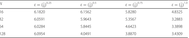
Table 5Rate of convergence for Example 2
N ε¼ ð1
NÞ 0:25
ε¼ ð1 NÞ
0:5
ε¼ ð1 NÞ
0:75
ε¼ ð1 NÞ
1:0
16 6.1820 6.1562 5.8280 4.8325
32 6.0591 5.9643 5.3567 3.2883
64 6.0284 5.8445 4.6423 3.3898
and sixth-order methods. Hence, the Richardson extrapolation method accelerates
fourth order into sixth order convergent as given in Table 2. The results in Tables 3
and 5further confirmed that the computational rate of convergence and theoretical
es-timates are in agreement (Tables 4and5). Generally, the present method is consistent,
is stable, and gives more accurate numerical solution for solving second-order self-adjoint singularly perturbed boundary value problems.
Acknowledgements
The authors wish to express their thanks to the authors of literatures for the provided scientific aspects and idea for this work. Also, we request to express great thanks to reviewers for the constructive comments and inputs given to improve the quality of our work.
Authors’contributions
MKS raised the first idea on the stated title and wrote, analyzed and interpreted the data. GFD modified the title so as to make it workable, edited, analyzed and interpreted the data again in the well-organized form. TAB accomplished the numerical computation of the solution for the governing differential equations of the present problem using MATLAB software and display results in tables and graphs. All authors read and approved the final manuscript.
Funding
Not applicable
Availability of data and materials
All data generated or analyzed during this study are included.
Competing interests
The authors declare that they have no competing interests.
Received: 5 June 2019 Accepted: 9 October 2019
References
1. Delkhon, M, Delkhosh, M: Analytic solution of some self-adjoint equations by using variable change method and its application, J Appl Math, 2012, 1-7 (2012), http://dx.doi.org/https://doi.org/10.1155/2012/180806.
2. Miller, HJJ, O’Riordan, E, Shishkin IG: Fitted numerical methods for singular perturbation problems, Error estimate in the maximum norm for linear problems in one and two dimensions, World Scientific. ISBN: 981-02-2462-1, (1996). 3. Suayip, Y., Niyazi, S.: Numerical solutions of singularly perturbed one-dimensional parabolic convection–diffusion
problems by the Bessel collocation method. Appl Math Comput.220, 305–315 (2013)
4. Roos, GH, Stynes, M, Tobiska, L: Robust numerical methods for singularly perturbed differential equations, Convection-diffusion-reaction and flow problems, Springer-Verlag Berlin Heidelberg, Second Edition, (2008).
5. Mishra, H.K., Kumar, M., Singh, P.: Initial-value Technique for self-adjoint singular perturbation boundary value problems. Comput Math Model.20, 207–218 (2009)
6. Rashidinia, J., Mohammadi, R., Moatamedoshariati, S.H.: Quintic spline method for solution of singularly perturbed boundary value problems. Int J Comput Meth Eng Sci Mech.11, 247–257 (2010)
7. Tirmizi, A.I., Haq, F.I., Islam, S.: Non-polynomial spline solution of singularly perturbed boundary value problems. Appl Math Comput.196, 6–16 (2008)
8. Rashidinia, J., Mahmoodi, Z., Ghasemi, M.: Cubic spline solution of singularly perturbed boundary value problems with significant first derivatives. Appl Math Comput.190, 1762–1766 (2005)
9. Kadalbajoo, MK, Kumar, D: Variable mesh finite difference method for self-adjoint singularly perturbed two-point boundary value problems, J Comput Math, (2010) doi:https://doi.org/10.4208/ jcm.1003-m2809.
10. Kadalbajoo, M.K., Aggrwal, V.K.: Fitted mesh B-spline collocation method for solving self-adjoint singularly perturbed boundary value problems. Appl Math Comput.161, 973–987 (2005)
11. Munyakazi, J.B.: Higher order numerical methods for singular perturbation problems, PhD thesis. University of the Western Cape, South Africa (2009)
12. Fasika, W.G., Gemechis, F.D., Tesfaye, A.B.: Tenth order compact finite difference method for solving singularly perturbed 1D reaction - diffusion equations. Int J Eng Appl Sci (IJEAS).8, 15–24 (2016)
13. Fasika, W.G., Gemechis, F.D., Tesfaye, A.B.: Sixth-order compact finite difference method for singularly perturbed 1D reaction diffusion problems. J Taibah Univ Sci.11, 302–308 (2017)
14. Fasika, W., Gemechis, F., Tesfaye, A.: Fourth order compact finite difference method for solving singularly perturbed 1D reaction diffusion equations with dirichlet boundary conditions. Momona Ethiop J Sci (MEJS).8, 168–181 (2016) 15. Feyisa, E., Gemechis, F.: Higher order compact finite difference method for singularly perturbed one dimensional
reaction diffusion problems. J Niger Math Soc.36, 491–502 (2017)
16. Terefe, A., Gemechis, F., Tesfaye, A.: Fourth-order stable central difference method for self-adjoint singular perturbation problems. Ethiop J Sci Technol.9, 53–68 (2016)
17. Yitbarek, Z., Gemechis, F., Tesfaye, A.: Sixth-order stable central difference method for self-adjoint singular perturbation problems. Ethiop J Educ Sc.13, 23–41 (2017)
19. Kadalbajoo, M.K., Reddy, Y.N.: A non-asymptotic method for general singular perturbation problems. J Optimization Appl.55, 256–269 (1986)
20. Smith, GD: Numerical solution of partial differential equations, Finite difference methods, Third edition, Oxford University Pres, New York (1985).
Publisher’s Note