Simulation of floating potentials in industrial applications by boundary element methods

R E S E A R C H

Open Access

Simulation of floating potentials in industrial

applications by boundary element methods

Dominic Amann

_{, Andreas Blaszczyk}

_{, Günther Of}

_{and Olaf Steinbach}

*_{Correspondence: [email protected]} 1_{Institut für Numerische}

Mathematik, Technische Universität Graz, Steyrergasse 30, Graz, 8010, Austria

Full list of author information is available at the end of the article

Abstract

We consider the electrostatic field computations with floating potentials in a multi-dielectric setting. A floating potential is an unknown equipotential value associated with an isolated perfect electric conductor, where the flux through the surface is zero. The floating potentials can be integrated into the formulations directly or can be approximated by a dielectric medium with high permittivity. We apply boundary integral equations for the solution of the electrostatic field problem. In particular, an indirect single layer potential ansatz and a direct formulation based on the Steklov-Poincaré interface equation are considered. All these approaches are discussed in detail and compared for several examples including some industrial applications. In particular, we will demonstrate that the formulations involving constraints are vastly superior to the penalized formulations with high permittivity, which are widely used in practice.

MSC: 65N38; 78A30

Keywords: electrostatic field computations; boundary element methods; industrial applications

1 Introduction

For the solution of D electrostatic field problems, boundary element methods are widely used and are, in particular, advantageous in the presence of an unbounded domain. In ad-dition to Dirichlet and Neumann boundary conad-ditions, so-called floating potentials may occur. Isolated perfect electric conductors result in equipotential surfaces. The equipoten-tial value of the surface is unknown, but, in addition, the flux through the closed surface must be zero in the absence of sources. Such floating electrodes are found in, e.g., some lightning protection systems and can modify the breakdown probability of air gaps [].

While there are numerous papers on the solution of electrostatic field problems with floating potentials by boundary element methods and related methods, like the charge simulation method [, ], in the engineering literature, a detailed view based on a mathe-matically profound basis seems to be missing. In this paper, we try to close this gap and, in addition, compare several formulations in practical examples. In particular, we con-sider boundary element methods, see, e.g., [–], for the solution of electrostatic field problems with floating potentials in a multi-dielectric setting. We apply an indirect ap-proach based on the single layer potential and a domain decomposition method based on symmetric approximations of the local Dirichlet to Neumann maps, the so-called Steklov-Poincaré operators, see e.g. [–]. These two methods have been compared for

tostatic problems in [, ]. Here, we apply these formulations for electrodes at floating potentials.

As electrodes at floating potentials can be considered equivalent to dielectric bodies with infinite permittivity, a common strategy is to substitute electrodes at floating poten-tial by a dielectric media with high permittivity, see e.g. []. This approximation can be interpreted as a penalty approach. We compare this strategy to the direct incorporation of the constant but unknown potential and of the zero flux constraint into the formula-tions. While the penalty approach of a dielectric media with high permittivity needs no additional implementation work in a code which can cope with jumping permittivities, the approach with constraints is highly preferable from a mathematical point of view. Our numerical examples will demonstrate that the results of the approach with constraints are superior to the ones of the penalty approach. In addition, we will show that the formu-lations based on the Steklov-Poincaré interface equation have advantages over the single layer potential ansatz in case of corners and edges.

The paper is organized as follows: A model problem of the electrostatic field compu-tation with floating potential is introduced in Section . In Section , the formulations based on the Steklov-Poincaré interface equation and the single layer potential ansatz are presented, and the unique solvability of the variational formulations is proven. The boundary element discretization of both formulations is described in Section , and first academic examples in Section  show the advantages and disadvantages of the consid-ered approaches. Finally we discuss several extensions of the model problem and apply the methods to examples of industrial applications like an arrester, a bushing, and an in-sulator with partial wetting in Section .

2 Floating potentials in electrostatic field problems

We apply the scalar potential ansatz for the computation of an electrostatic fieldE= –∇ϕ. We consider the union=E∪F∪Dof several disjoint Lipschitz domains, a domain Eof an electrode, a domainF with a floating potential, and a dielectric domainD. In addition we define the exterior domainc_=R_\

. For the ease of presentation we

assume that the intersection of the closures of any two domainsE,F, andDis empty. We will comment on more general situations in Section . The model problem reads: Find a scalar potentialϕsuch thatϕD=ϕ|D,ϕ=ϕ|c_, and a constantα=ϕ|Fare the solution of

–ϕD(x) =  forx∈D, ()

–ϕ(x) =  forx∈c, ()

ϕ(x) =g forx∈E:=∂E, ()

ϕD(x) =ϕ(x) forx∈D, ()

εD ∂ ∂nD

ϕD(x) =ε

∂ ∂nD

ϕ(x) forx∈D, ()

ϕ(x) =O

|x|– as|x| → ∞, ()

ϕ(x) =α forx∈F:=∂F, ()

F ∂ ∂nF

Herenidenotes the exterior unit normal vector oni:=∂i,i∈ {,D,E,F}, and is defined almost everywhere. On the surfaceEof the electrode a constant potentialgis given in (), while we enforce continuity of the potential as well as of the flux for the dielectrics by () and (). In addition, we introduceas the union of all boundaries. For our simple model

problem=. Note that we distinguish and from the beginning, such that the

developed boundary integral equations can be applied to more general settings which are discussed in Section . The dielectric domain is characterized by its relative permittivity εDand the exterior domaincbyε. For the floating potential, we assume a constant but

unknown potentialαon the boundaryF in (), but the total flux through this surface is zero, see ().

We will consider two approaches to solve such boundary value problems with a floating potential numerically. The first approach is to solve the boundary value problem in the form ()-(), taking into account the constant but unknown potentialαand the constraint () directly. The second approach, which is widely used in practice due to its simple im-plementation, is to approximate the floating potential by consideringFto be a dielectric medium with high relative permittivityεF, i.e., to determine a potentialϕF instead ofα. In this case we end up with a system consisting of ()-() with additional transmission conditions onF:

ϕF(x) =ϕ(x) forx∈F, ()

εF ∂ ∂nF

ϕF(x) =ε

∂ ∂nF

ϕ(x) forx∈F. ()

We will demonstrate by some numerical examples in Section  that the penalty approach of an additional dielectric medium with a high relative permittivity gives bad approxima-tions of the floating potential in general.

3 Boundary integral equations

If we useC=\E=D∪F instead ofD in () and () and set the permittivitiesε correctly, the model with a high relative permittivityεFis the special case ()-() of the full model ()-() with a floating potential. Thus we will derive the boundary integral equations for the full model only. For the model with a high relative permittivity we just need to drop the boundary integral equations related toF and take into account the ones ofDforF in addition.

We consider an approach which is based on the Steklov-Poincaré interface equation known from domain decomposition methods, see e.g. [, ], and an indirect ansatz lead-ing to a slead-ingle layer boundary integral equation. While the latter approach is popular due to the ease of implementation, the domain decomposition approach will result in better approximations for the examples in Sections  and .

3.1 Steklov-Poincaré interface equation

The solutions of the Laplace equations () and () are given by the representation formulae

ϕD(x) =

D

U∗(x,y)tD(y)dsy–

D ∂ ∂nD,y

U∗(x,y)ϕD(y)dsy forx∈D,

ϕ(x) = –



U∗(x,y)t(y)dsy+



∂ ∂n,y

withtD:=∂∂nDϕD,t:= ∂

∂nϕ, and the fundamental solution

U∗(x,y) =  π



|x–y|.

Thus we need to determine the unknown parts of the Cauchy data [ti,ϕi],i∈ {,D}. The interior Steklov-Poincaré operator SD _:H/₍

D)→H–/(D) maps some given Dirichlet datum ϕD onto the related Neumann datumtD=SDϕD of the corresponding solution of the Laplace equation (). Analogously the exterior Steklov-Poincaré operator S_:H/₍

)→H–/() givest= –Sϕ. These two operators can be defined in their

so-called symmetric representation, see e.g. [, Section .., p. ], by

SD=DD+

 I+K

D

V_D–

 I+KD

,

S_=D +

 I–K

 V–   I–K

.

The single layer boundary integral operatorVi, the double layer boundary integral oper-atorKi, its adjointKi, and the hypersingular operatorDiare defined with respect toi, i∈ {,D,E,F}, by

(Viti)(x) =

i

U∗(x,y)ti(y)dsy,

(Kiϕi)(x) =

i ∂ ∂ni,y

U∗(x,y)ϕi(y)dsy,

K_iti

(x) =

i ∂ ∂ni,x

U∗(x,y)ϕi(y)dsy,

(Diϕi)(x) = – ∂ ∂ni,x

i ∂ ∂ni,y

U∗(x,y)ϕi(y)dsy.

As the two Steklov-Poincaré operatorsSD andS correspond to the solution of local Dirichlet boundary value problems, it remains to satisfy the boundary and transmission conditions. We need to find a global functionϕ∈H/_{() such that}

ϕ(x) =g forx∈E, ϕ(x) =α forx∈F,

i.e., the boundary conditions () and () as well as the transmission condition () are satis-fied. Usingt= –Sϕ,tD=SDϕ|D, and the splittingϕ=ϕD+gE+αF, where i(x) =  for x∈iand  else, the remaining transmission condition () and the constraint () result in the final system: FindϕD∈H/(D) andα∈Rsuch that

εDSD+εS

ϕD(x) +αε

SF

(x) = –gε

SE

(x) forx∈D, ()

F

SϕD

(x) +αSF

(x)dsx= –g

F

SE

3.2 Single layer boundary integral operator formulation

Due to its popularity in practice, see [] and references given therein, we consider a global single layer potential ansatz by

ϕ(x) =

U∗(x,y)w(y)dsy forx∈R\

for any single layer charge densityw∈H–/_{() for the global solutionϕof the}

bound-ary value problem ()-(). With this choice the local partial differential equations () and (), the continuity condition () as well as the radiation condition () are satisfied. The remaining Dirichlet boundary condition (), the floating potential condition (), the flux transmission condition (), and the scaling condition () provide the equations to deter-mine the unknown densityw∈H–/_():

(Vw)(x) =g forx∈E, ()

(Vw)(x) –α=  forx∈F, ()

 

εD+ε

εD–ε

w(x) +Kw(x) =  for almost allx∈D, ()

F

– w(x) +

Kw(x)

dsx= , ()

whereV denotes the global single layer boundary integral operator andKis the global adjoint double layer boundary integral operator forx∈:

(Vw)(x) =

U∗(x,y)w(y)dsy,

Kw(x) =

∂ ∂nx

U∗(x,y)w(y)dsy.

3.3 Unique solvability

Lemma . There exists a unique solution(ϕD,α)∈H/(D)×Rsatisfying()-(). Proof Using the splittingϕ=ϕD+αF+gE, we can reformulate ()-() as: Findϕ∈X:=

{ψ∈H/_{() :ψ}

|F=α,α∈R,ψ|E= }:

εDSD+εS

ϕ,ψ= –gεSE,ψ

for allψ∈X.

This variational formulation admits a unique solution, as X ⊂ H/_{(), the exterior}

Steklov-Poincaré operatorS_isH/_{()-elliptic, and the interior Steklov-Poincaré}

oper-atorSD_isH/₍

D)-semi-elliptic, see, e.g., [, Lemma ., p. f] and [, Section ..,

p.].

Lemma . Let(ϕD,α)∈H/(D)×Rbe a solution of the Steklov-Poincaré interface equa-tions()-(),and let w∈H–/_{()be a solution of the indirect single layer approach}

()-().Then there holds the relation

ϕ(x) =ϕD(x) +αF(x) +gE(x) = (Vw)(x) for x∈.

equation. OnFthe assertion holds true due to (). OnDwe start from the continuity () of the flux for the single layer potential approach, usew=V–_{Vwand the symmetry}

relationKV–_=V–_{K, see e.g. [, Corollary ., p.],}

 =εD

 I+K

_{w(x) +ε}



 I–K

_w(x)

=εDV–

 I+K

Vw(x) +εV–

 I–K

Vw(x) forx∈D.

For the first termu=V–₍

I+K)zwe can apply some simplifications using the splitting

of the functions and operators

(VDuD)(x) + (VEuE)(x) + (VFuF)(x)

=

zD(x) + (KDzD)(x) + (KEzE)(x) + (KFzF)(x)

for almost allx∈D, which reduces to

(VDuD)(x) =

 I+KD

zD(x) for almost allx∈D

because there holds

(Viti)(x) – (Kizi)(x) =  forx∈ci,i∈ {E,F},

for any solutionzi andti=∂∂znii of the local Laplace equations. With the so-called non-symmetric representations SD _=V–

D (I+KD) and S=V–(I–K) of the

Steklov-Poincaré operators we end up with

εDSD(Vw)(x) +εS(Vw)(x) =  forx∈D.

Applying the same technique for the constraint () of the single layer potential ansatz, we end up with

F

S(Vw)(x)dsx= .

Taking into account the floating potential (), these two equations coincide with the formulation ()-() of the Steklov-Poincaré interface equation, and hence we conclude

ϕ=Vwon.

Due to equivalence of the two formulations we conclude the unique solvability of the indirect approach ()-() from Lemma ..

4 Boundary element methods

For the discretization of the considered boundary integral formulations, we assume a

quasi-uniform mesh of the surface withNplane triangles andMnodes. The

use Galerkin variational formulations for the discretization of the domain decomposition method ()-() and of the single layer boundary integral equations ()-().

4.1 Steklov-Poincaré interface equation

We transfer the splitting ϕ=ϕD+αF +gE of the solution of ()-() to the Steklov-Poincaré operators such that S_ij indicates that the operatorSis applied to a function defined onjonly and evaluated onifori,j∈ {D,E,F}.

Thus the discrete Galerkin variational formulation of ()-() is to find (ϕD,h,α)∈ S

h(D)×Rsuch that

εDSDDD+εSDD

ϕD,h,vh

D+αε

S_DFF,vh

D= –εg

S_DEE,vh

D,

ε

S_FD ϕD,h, F

+αε

S_FFF, F

= –εg

S_FEE, F

for allvh∈S_h(D). Due to the inverse of the single layer potential, a direct computation of SandSDis not possible in general. But we can use the approximations

SD_h :=DD,h+



M

D,h+KD,h

V_D–_,h



MD,h+KD,h

,

S_h:=D,h+



M

,h–K,h

V_,–_h



M,h–K,h

.

These approximations are symmetric, positive semi-definite, and positive definite, re-spectively. The additional error caused by these approximations features the same quasi-optimal order of convergence as the Galerkin approximations of the exact operators, see e.g. [, Lemma .]. Thus, there is no substantial loss of accuracy. The Galerkin matrices are given by

Di,h[k,] =

Diψ,ψk

i, Vi,h[m,n] =

Viψn,ψm

i,

Ki,h[m,] =

Kiψ,ψm

i, Mi,h[m,] =

ψ,ψ_m i

fork,= , . . . ,Mi;m,n= , . . . ,Ni, andi∈ {D,E,F}. Finally, we have to solve the following system of linear equations

εDS_DDD _,h+εS_DD _,h a

a λ

ϕ D α

= fD

fF

, ()

where

a[] :=ε

S_DF,hF,ψ

D, λ:=ε

S_FF_,hF, F

F.

Due to the positive semi-definiteness ofSD

h and the positive definiteness ofShthe linear system () is uniquely solvable, see Lemma ..

linear equations

εDSDDD ,h+εSDD ,h εSDF,h εS_FD,h εFS_FFF _,h+εS_FF,h

ϕ D ϕ F

= fD

f F

. ()

The unique solvability of both discrete formulations () and () is a consequence of the positive definiteness of the approximationS

hof the exterior Steklov-Poincaré operatorS and the positive semi-definiteness of the approximationSi_hof the other Steklov-Poincaré operatorSi_{(i∈ {D,F}), see, e.g., [, Lemma ., p.f] and [, Lemma ., p.].}

4.2 Single layer boundary integral operator formulation

We use piecewise constant functions fromS_h() as test and ansatz functions in the sys-tem ()-(). As before we apply the splitting of the unknown densitywh∈Sh() into (wF,h,wE,h,wD,h)∈S_h(F)×S_h(E)×S_h(D). So the discrete variational formulation of the single layer boundary integral operator formulation ()-() is to find (wF,h,wE,h,wD,h,α)∈ S

h(F)×Sh(E)×Sh(D)×Rsuch that

VEFwF,h+VEEwE,h+VEDwD,h,ψEE=gE,ψEE,

VFFwF,h+VFEwE,h+VFDwD,h,ψFF–αF,ψFF= ,

K_DF wF,h+KDE wE,h+KDD wD,h,ψD

D+

 

εD+ε

εD–εwD,h,ψDD= ,

K_FF wF,h+KFE wE,h+KFD wD,h, F

F–



wF,h, FF= , () for all test functionsψi∈Sh(i) fori∈ {F,E,D}. In the considered geometric setting, the equation () allows for some simplification utilizing the adjointness and the kernel prop-erties of the double layer potential operator:

 =K_FF wF,h+KFE wE,h+KFD wD,h, F

F– 

wF,h, FF =wF,h,KFFFF–



wF,h, FF= –wF,h, FF.

This formulation is equivalent to the following system of linear equations

⎛ ⎜ ⎜ ⎜ ⎝

VEE,h VEF,h VED,h

VFE,h VFF,h VFD,h –b

K_DE,h K_DF,h  

εD+ε

εD–εMh+K

DD,h b ⎞ ⎟ ⎟ ⎟ ⎠ ⎛ ⎜ ⎜ ⎜ ⎝ w_E w_F w_D α ⎞ ⎟ ⎟ ⎟ ⎠= ⎛ ⎜ ⎜ ⎜ ⎝ f E    ⎞ ⎟ ⎟ ⎟ ⎠, () where

Vij,h[m,n] =

Vjψn,ψm

i, Kij,h[m,n] =

Kjψn,ψm

i,

Mij,h[m,n] =

ψ_n,ψ_m

i, b[m] =

ψ_m, F

F

For the approach which approximates the floating potential by consideringF as a di-electric with a high relative permittivityεF, the corresponding system reads

⎛ ⎜ ⎝

VEE,h VEF,h VED,h

K_{FE,h }εF+ε

εF–εMh+K

FF,h KFD,h

K_DE,h K_{DF,h }εD+ε

εD–εMh+K

DD,h ⎞ ⎟ ⎠

⎛ ⎜ ⎝

w_E w_F w_D

⎞ ⎟

⎠=

⎛ ⎜ ⎝ f

E  

⎞ ⎟

⎠. ()

To our best knowledge, the stability of these indirect boundary element formulations is still an open problem for general Lipschitz surfaces due to the inconsistent, but widely used discretization of the adjoint double layer potential inL().

5 Numerical examples

In this section, we consider a few rather academic examples to compare the introduced approaches to solve the electrostatic potential problem ()-(). We compare four formu-lations in total. We apply the Steklov-Poincaré (SP) operator formulation () and the in-direct single layer potential (SL) ansatz () for the full dielectric approach (full dielectric) with a high relative permittivityεF= , to approximate the floating potential. For the direct incorporation (floating) of the floating potential we solve the Steklov-Poincaré (SP) system () and the indirect single layer potential (SL) ansatz (), respectively.

For the computations, we used an implementation [] of the proposed boundary ele-ment methods which is based on the Fast Multipole Method [] for fast and data-sparse realizations of the involved boundary integral operators. The Steklov-Poincaré operator formulation is implemented by means of MPI and we used one process per active sub-domain, i.e. two processes for () and three processes for (). The implementation of the Fast Multipole Method utilizes OpenMP and we used two threads for each instance of the program. The computations were done on a Workstation with  Intel Xeon E processors and  GB RAM.

We use the concept of operators of opposite order [] for the preconditioning of the Steklov-Poincaré operator formulations () and (). We apply the artificial multilevel preconditioning [, ] for the inner inversion of the Galerkin matrix of the single layer boundary integral operator in the Steklov-Poincaré operator formulations. For the systems () and () of the indirect single layer potential ansatz, we use the artificial multilevel preconditioning for the block of the single layer boundary integral operator and a diagonal scaling for the block of the adjoint double layer potential operator.

5.1 Two spheres

The two spheres of our first example [] have the same diameter which is twice the dis-tance of the two spheres. The first sphere E is an electrode with a given potential of ϕ=g=  on its surface. The second sphereF is either a floating potential or a dielec-tric with relative permittivityεF = ,, depending on the considered approach. The surrounding air has the relative permittivityε= .

Table 1 Approximate values of the floating potentialαonFand computational times for

the example of two spheres

Number of elements 256 1,040 4,160

SP floating 32.41 1 s 33.63 8 s 33.86 35 s

SL floating 32.41 1 s 33.63 4 s 33.86 20 s

SP full dielectric 32.40 2 s 33.62 12 s 33.85 50 s

SL full dielectric 32.39 1 s 33.62 5 s 33.86 28 s

2D ELFI 33.9

Table 2 Approximate values of the floating potentialαonFand computational times for

the example of a sphere and a bicone

Number of elements 384 1,536 6,144 24,576

SP floating 44.512 2 s 45.339 15 s 45.572 79 s 45.637 329 s

SL floating 44.512 2 s 45.341 7 s 45.573 28 s 45.637 124 s

SP full dielectric 44.512 3 s 45.340 27 s 45.573 106 s 45.636 569 s SL full dielectric 44.433 2 s 45.355 11 s 45.553 34 s 45.632 168 s

2D ELFI 45.7

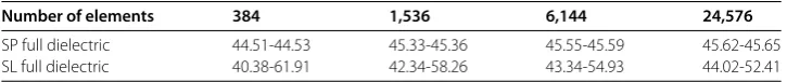
Table 3 Range of the floating potentialϕFfor the sphere and the bicone

Number of elements 384 1,536 6,144 24,576

SP full dielectric 44.51-44.53 45.33-45.36 45.55-45.59 45.62-45.65 SL full dielectric 40.38-61.91 42.34-58.26 43.34-54.93 44.02-52.41

directly but provide the mean value of the potential onF. Even on the finest refinement level the potentialϕFis not constant, it has a range of . for the indirect approach and . for the Steklov-Poincaré operator formulation.

We notice that all four formulations result in good and similar approximate solutions. Only the indirect single layer formulation () for the full dielectric model gives a potential which is not quite constant although we consider approximations of smooth objects. We will encounter this behavior to a greater extend in the next example.

5.2 Sphere and bicone

Now we consider an example consisting of a sphere and a bicone []. Both have the same diameter and are arranged at a distance of one eighth of their diameter. One spike of the bicone points towards the sphere. The sphereE is an electrode with a given potential ϕ=g= . The biconeF has a floating potential and the exterior domain has a relative permittivity ofε= . In Table , we present the approximations of the floating potential

α and the computational times. Again an approximate solution of the potential on the surfaceF of the cone by an axial symmetric FEM solver is used for comparison.

equation are higher than those of the single layer potential ansatz for the same mesh, but we neglect the accuracy of the approximations (see results for ‘SL full dielectric’ in Table ) in this comparison.

6 Extensions and applications

We observed poor approximations by the single layer potential ansatz for large jumps in the permittivitiesεin the example of the sphere and the bicone due to artificial singular-ities in the discrete solution, see the formulation ‘SL full dielectric’ in Table . For such simple examples the single layer potential ansatz with direct realization of the floating potential (‘SL floating’) gives still good results. But for examples with large jumps of the coefficientsεD andεthis is not the case anymore. As the third row in () is similar to

the second and third row in (), we are facing the same problem as for the formulation ‘SL full dielectric’ in Table . We observed these problems with artificial singularities in the discrete solution in the presence of dielectric media already for relative permittivity εDof  and higher, see e.g. [, ].

But for more general examples we have to cope with such jumps in the relative permit-tivities. In such cases, the approximation error of the single layer approach is more than one order of magnitude larger than the one of the Steklov-Poincaré operator formulations for the same mesh, see [, ]. Thus one needs significantly finer meshes for the single layer potential ansatz to come up with the same accuracy for this class of problems. This results in larger computational times than for the Steklov-Poincaré operator formulations. Due to these significant drawbacks of the single layer potential ansatz, we will consider the Steklov-Poincaré operator formulations only.

For real world examples, we need to consider more general settings. For the ease of presentation we have restricted the description of the formulations to one representative of each kind of subdomains and to well separated subdomains. We will now comment on some extensions.

The extension to several electrodes and dielectric subdomains is straightforward. For each boundaryFiandDithe corresponding boundary integral equations (), (), and ()-(), respectively, have to be considered separately. For each floating subdomainFi a separate degree of freedomαiand the corresponding constraint

_Fi ∂ ∂nFi

ϕ(x)dsx= 

have to be incorporated.

If two subdomains are in contact, we have to make some additional modifications. If a dielectric subdomain is in contact with an electrode, we use a discrete extensiongof the given potentialgto the surfaceDof the dielectric and determine the unknown remainder ϕD–gofϕD. If the floating potential is surrounded by a dielectric medium instead of the exterior air domain the vectoraand the coefficientλin () involveεDSDinstead ofεS.

In (),εDSDandεSare interchanged.

IfFhas interfaces to more than one subdomain, the constraint of the floating potential has to be taken with care. In the case of an interface toDand to the exterior domainc,

the constraint reads as

εD

F∩D ∂ ∂nF

ϕD(x)dsx+ε

F∩

∂ ∂nF

Figure 1 IEC arrester: the gray shades indicate the subdomains.

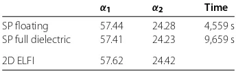
Table 4 Approximate values of the floating potentials and computational times for the IEC arrester

α1 α2 Time

SP floating 57.44 24.28 4,559 s SP full dielectric 57.41 24.23 9,659 s

2D ELFI 57.62 24.42

This extended constraint can be transferred straightforward to the approach of the Steklov-Poincaré interface equation by the means of the related Steklov-Poincaré oper-ators. For the indirect single layer potential ansatz, the simplification of the related con-straint () seems not to be possible in general.

6.1 IEC arrester

The two remaining Steklov-Poincaré operator formulations are compared for the compu-tation of the electric potential of the IEC surge arrester [, Annex L] shown in Figure . Each of the three sections of the arrester (gray) consists of a metal-oxide cylindrical col-umn with the equivalent relative permittivityεD=  surrounded by a porcelain housing with the relative permittivityεD= . In between the two dielectric domains there is a layer of air. The three sections are separated by two metal flanges (dark gray) at floating poten-tials. At the light gray parts the potential is given. The pedestal and the large surrounding cylinder are grounded electrodes with potentialϕGND= . The top high voltage lead and

the toroidal grading ring are electrodes with potentialϕHV= . The exterior domain and

the air inside the porcelain housing are modeled as dielectrics withε= .

Figure 2 Geometric settings of (a) the bushing and (b) the partially wet insulator.

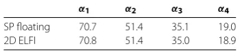
Table 5 Approximate values of the floating potentials for the bushing

α1 α2 α3 α4

SP floating 70.7 51.4 35.1 19.0

2D ELFI 70.8 51.4 35.0 18.9

6.2 Bushing

The next example models a high voltage bushing [] shown in Figure (a). It consists of a cylindrical conductor (light gray) with potentialϕHV=  surrounded by five thin

metallic foils embedded in a solid dielectric material (gray) with the relative permittivity εD= . The most outer foil (light gray) is groundedϕGND=  while the other four foils (dark

gray) are at floating potentials. The role of the floating foils is enforcing a uniform poten-tial distribution along the conical surface of the bushing. The difficult aspect of modeling bushings is the small thickness of the foils: for the bushing in Figure (a) the ratio between the foil thickness and its axial length is in the range of –_{. The computational mesh}

con-sists of , global nodes. Consequently the distance between elements created on the parallel foil surfaces is approximately  times smaller than the size of the elements. In spite of these extreme geometrical relations the floating potentials calculated for all foils with the Steklov-Poincaré operator approach show a good agreement with the D solu-tion as presented in Table . The system () of linear equasolu-tions is solved in  steps of a preconditioned CG method to a relative accuracy of –_.

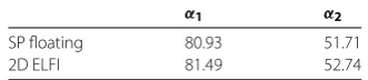
6.3 Insulator with partial wetting

The last example as depicted in Figure (b) is an insulator with embedded electrodes (light gray) at potentialsϕHV=  andϕGND= . The relative permittivity of the insulator (gray)

isεD= . The upper surface of both insulator sheds is covered by a water layer (dark gray). For the operational frequency of - Hz water behaves like a conducting material and can be approximated for a capacitive electrostatic field computation as an electrode. Con-sequently, the two very thin domains of water (dark gray) on the insulator sheds are mod-eled as electrodes at floating potentials. The geometrical dimensions of this arrangement are given in Table .

Table 6 Geometrical dimensions of the insulator with partial wetting

Quantity In mm

Electrodes distance 14

Insulation thickness between electrode and air 5

Shed diameter 160

Shed thickness 6

Water layer thickness 1

Table 7 Approximate values of the floating potentials for the insulator with partial wetting

α1 α2

SP floating 80.93 51.71

2D ELFI 81.49 52.74

7 Conclusions

We insistently recommend the formulations which integrate the floating potential directly and the zero flux condition by a constraint. These formulations give better results and are faster than the approximation obtained by a dielectric media with high permittivity because of a smaller number of degrees of freedom and a smaller number of steps of the iterative solver. Thus the additional effort for the implementation of the modified system pays off.

In case of no or small jumps of the permittivity, the indirect approach by the single layer potential and the direct formulation based on the Steklov-Poincaré interface equation give good results. Here the computational times of the single layer approach are smaller.

In case of larger jumps of the permittivity, the direct formulation based on the Steklov-Poincaré interface equation turned out to be superior to the indirect single layer potential ansatz, as the results are of much better quality. In particular, the indirect approach shows unphysical singularities close to edges and corners in the case of large jumps of the per-mittivity. Comparing the computational times for a desired accuracy and not for a fixed mesh the Steklov-Poincaré formulations turns out to be faster.

Competing interests

The authors declare that they have no competing interests.

Authors’ contributions

All authors contributed equally to the writing of this paper. All authors read and approved the final manuscript.

Author details

1_{Institut für Numerische Mathematik, Technische Universität Graz, Steyrergasse 30, Graz, 8010, Austria.}2_Corporate

Research, ABB Switzerland Ltd., Baden-Dättwil, 5405, Switzerland.

Acknowledgements

This work was supported by the FP7 Marie Curie IAPP Project CASOPT (Controlled Component and Assembly Level Optimisation of Industrial Devices, www.casopt.com).

Received: 17 April 2014 Accepted: 12 October 2014 Published:30 Oct 2014 References

1. Roman F, Cooray V, Scuka V:Comparison of the breakdown of rod-plane gaps with floating electrode.IEEE Trans. Dielectr. Electr. Insul.1998,5(4):622-624.

2. Blaszczyk A, Steinbigler H:Region-oriented charge simulation.IEEE Trans. Magn.1994,30(5):2924-2927. 3. Singer H, Steinbigler H, Weiss P:A charge simulation method for the calculation of high voltage fields.IEEE Trans.

Power Appar. Syst.1974,93(5):1660-1668.

4. Hsiao GC, Wendland WL:Boundary Integral Equations. Berlin: Springer; 2008. [Applied Mathematical Sciences, vol. 164.] 5. Sauter SA, Schwab C:Boundary Element Methods. Berlin: Springer; 2011. [Springer Series in Computational Mathematics,

6. Steinbach O:Numerical Approximation Methods for Elliptic Boundary Value Problems. Finite and Boundary Elements. New York: Springer; 2008.

7. Carstensen C, Kuhn M, Langer U:Fast parallel solvers for symmetric boundary element domain decomposition equations.Numer. Math.1998,79(3):321-347.

8. Hsiao GC, Steinbach O, Wendland WL:Domain decomposition methods via boundary integral equations.

J. Comput. Appl. Math.2000,125(1-2):521-537.

9. Hsiao GC, Wendland WL:Domain decomposition in boundary element methods. InFourth International Symposium on Domain Decomposition Methods for Partial Differential Equations, Proc. Symp., Moscow/Russ. 1990. Philadelphia: SIAM; 1991:41-49.

10. Hsiao GC, Wendland WL:Domain decomposition via boundary element methods. InNumerical Methods in Engineering and Applied Sciences, Part I. Edited by Alder H, Heinrich JC, Lavanchy S, Onate E, Suarez B. Barcelona: CIMNE; 1992:198-207.

11. Andjelic Z, Of G, Steinbach O, Urthaler P:Boundary element methods for magnetostatic field problems: a critical view.Comput. Vis. Sci.2011,14:117-130.

12. Andjelic Z, Of G, Steinbach O, Urthaler P:Fast boundary element methods for industrial applications in magnetostatics. InFast Boundary Element Methods in Engineering and Industrial Applications. Edited by Langer U, Schanz M, Steinbach O, Wendland WL. Berlin: Springer; 2012:111-143. [Lecture Notes in Applied and Computational Mechanics, vol. 63.]

13. Konrad A, Graovac M:The finite element modeling of conductors and floating potentials.IEEE Trans. Magn.1996,

32(5):4329-4331.

14. Pechstein C:Finite and Boundary Element Tearing and Interconnecting Solvers for Multiscale Problems. Berlin: Springer; 2013. [Lecture Notes in Computational Science and Engineering, vol. 90.]

15. Toselli A, Widlund O:Domain Decomposition Methods - Algorithms and Theory. Berlin: Springer; 2005. [Lecture Notes in Computational Mathematics, vol. 34.]

16. Andjeli´c Z, Smaji´c J, Conry M:BEM-based simulations in engineering design. InBoundary Element Analysis. Berlin: Springer; 2007:281-352. [Lect. Notes Appl. Comput. Mech., vol. 29.]

17. Of G, Steinbach O, Wendland WL:The fast multipole method for the symmetric boundary integral formulation.

IMA J. Numer. Anal.2006,26(2):272-296.

18. Greengard L, Rokhlin V:A fast algorithm for particle simulations.J. Comput. Phys.1987,73:325-348. 19. Steinbach O, Wendland WL:The construction of some efficient preconditioners in the boundary element

method.Adv. Comput. Math.1998,9(1-2):191-216.

20. Steinbach O:Artificial multilevel boundary element preconditioners.Proc. Appl. Math. Mech.2003,3:539-542. 21. Of G:An efficient algebraic multigrid preconditioner for a fast multipole boundary element method.Computing

2008,82(2-3):139-155.

22. Blaszczyk A:Region-oriented BEM formulation for numerical computation of electric fields. InScientific Computing in Electrical Engineering SCEE2008. Edited by Roos J, Costa LRJ. Berlin: Springer; 2010:69-76. [Mathematics in Industry, vol. 14.]

23. Andjelic Z, Kristajic B, Milojkovic S, Blaszczyk A, Steinbigler H, Wohlmuth M:Integral methods for the calculation of electric fields, for application in high voltage engineering.Technical report10, Scientific Series if the International Bureau, Forschungszentrum Jülich; 1992.

24. International Electrotechnical Commission: IEC Technical Standard 60099-4:Surge Arresters - Part 4: Metal-Oxide Surge Arresters Without Gaps for A.C. Systems. 2.2 edition; 2009.

10.1186/2190-5983-4-13