On: 03 May 2015, At: 17:33
Publisher: Taylor & Francis
Informa Ltd Registered in England and Wales Registered Number: 1072954 Registered
office: Mortimer House, 37-41 Mortimer Street, London W1T 3JH, UK
Click for updates
GIScience & Remote Sensing
Publication details, including instructions for authors and
subscription information:
http://www.tandfonline.com/loi/tgrs20
Spatial data, analysis approaches,
and information needs for spatial
ecosystem service assessments: a
review
Margaret E. Andrew
a, Michael A. Wulder
b, Trisalyn A. Nelson
c&
Nicholas C. Coops
da
School of Veterinary and Life Sciences, Murdoch University,
Murdoch, Western Australia, Australia
b
Canadian Forest Service (Pacific Forestry Centre), Natural
Resources Canada, Victoria, British Columbia, Canada
cSpatial Pattern Analysis and Research (SPAR) Laboratory,
Department of Geography, University of Victoria, Victoria, British
Columbia, Canada
d
Department of Forest Resource Management, University of
British Columbia, Vancouver, British Columbia, Canada
Published online: 01 May 2015.
To cite this article: Margaret E. Andrew, Michael A. Wulder, Trisalyn A. Nelson & Nicholas
C. Coops (2015) Spatial data, analysis approaches, and information needs for spatial
ecosystem service assessments: a review, GIScience & Remote Sensing, 52:3, 344-373, DOI:
10.1080/15481603.2015.1033809
To link to this article:
http://dx.doi.org/10.1080/15481603.2015.1033809
PLEASE SCROLL DOWN FOR ARTICLE
Taylor & Francis makes every effort to ensure the accuracy of all the information (the
“Content”) contained in the publications on our platform. Taylor & Francis, our agents,
and our licensors make no representations or warranties whatsoever as to the accuracy,
completeness, or suitability for any purpose of the Content. Versions of published
independently verified with primary sources of information. Taylor & Francis shall not be
liable for any losses, actions, claims, proceedings, demands, costs, expenses, damages,
and other liabilities whatsoever or howsoever caused arising directly or indirectly in
connection with, in relation to or arising out of the use of the Content.
This article may be used for research, teaching, and private study purposes. Terms &
Conditions of access and use can be found at
http://www.tandfonline.com/page/terms-and-conditions
It is essential that you check the license status of any given Open and Open
Select article to confirm conditions of access and use.
Spatial data, analysis approaches, and information needs for spatial
ecosystem service assessments: a review
Margaret E. Andrewa, Michael A. Wulderb*, Trisalyn A. Nelsoncand Nicholas C. Coopsd
a
School of Veterinary and Life Sciences, Murdoch University, Murdoch, Western Australia, Australia;bCanadian Forest Service (Pacific Forestry Centre), Natural Resources Canada, Victoria, British Columbia, Canada;cSpatial Pattern Analysis and Research (SPAR) Laboratory, Department of Geography, University of Victoria, Victoria, British Columbia, Canada;dDepartment of Forest Resource Management, University of British Columbia, Vancouver, British Columbia, Canada
(Received 29 December 2014; accepted 23 March 2015)
Operational use of the ecosystem service (ES) concept in conservation and planning requires quantitative assessments based on accurate mapping of ESs. Our goal is to review spatial assessments of ESs, with an emphasis on the socioecological drivers of ESs, the spatial datasets commonly used to represent those drivers, and the methodo-logical approaches used to spatially model ESs. We conclude that diverse strategies, integrating both spatial and aspatial data, have been used to map ES supply and human demand. Model parameters representing abiotic ecosystem properties can be supported by use of well-developed and widely available spatial datasets. Land-cover data, often manipulated or subject to modeling in a GIS, is the most common input for ES modeling; however, assessments are increasingly informed by a mechanistic under-standing of the relationships between drivers and services. We suggest that ES assess-ments are potentially weakened by the simplifying assumptions often needed to translate between conceptual models and widely used spatial data. Adoption of quantitative spatial data that more directly represent ecosystem properties may improve parameterization of mechanistic ES models and increase confidence in ES assessments.
Keywords:ecosystem function; ecological processes; ecosystem services; spatial data; land cover; satellite
1. Introduction
It is now widely acknowledged that ecological systems, through ecosystem services (ESs), are important contributors to human livelihoods and well-being. Ecosystems provide natural resources with value to a wide range of sectors, many cultural values, essential life support services, and ecological processes supporting those varied services (Table 1; MEA2005). Despite the recent rapid increase in interest in ESs by scientists, policy-makers, conservation practitioners, and natural resource managers (Figure 1), adequate methods to spatially quan-tify ESs and plan for their continued provisioning remain scarce (Figure 1, and seeTable 2for
*Corresponding author. Email:[email protected]
Vol. 52, No. 3, 344–373, http://dx.doi.org/10.1080/15481603.2015.1033809
© 2015 Crown Copyright. Published by Taylor & Francis.
This is an Open Access article. Non-commercial re-use, distribution, and reproduction in any medium, provided the original work is properly attributed, cited, and is not altered, transformed, or built upon in any way, is permitted. The moral rights of the named author(s) have been asserted.
Permission is granted subject to the terms of the License under which the work was published. Please check the License conditions for the work which you wish to reuse. Full and appropriate attribution must be given. This permission does not cover any third party copyrighted material which may appear in the work requested.
a list of ES-related terms used in the text and their definitions). Operational use of ESs is limited by a general lack of ES indicators supported by existing data (Layke2009; Orians and Policansky2009); quantitative, spatial ES data products are rarer still. Yet, just as data on the distributions of species and communities drive prioritization exercises for biodiversity con-servation, spatial information on ESs is essential for effective planning. In addition, spatial assessments of ESs can reveal linkages between the supply of ESs and their users, as well as between individual services (Tallis and Polasky2009), and convey large amounts of informa-tion, increasing stakeholder awareness and engagement (Southern et al. 2011). Many researchers call for new or improved ES indicators (Carpenter et al.2009; de Groot et al.
2010; Feld et al. 2009, 2010) and spatially explicit assessments (Balmford et al. 2008; Cowling et al.2008; de Groot et al.2010; Tallis and Polasky2009; Meyerson et al.2005; Nicholson et al.2009) to identify areas within a planning region that are most important for sustaining a complete portfolio of ESs.
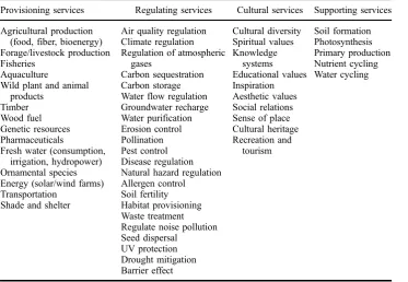
Research on ESs is a relatively recent and rapidly growing area (Figure 1). Our goal is to review studies that spatially assess ESs. To meet this goal, we reviewed nearly 150 (listed and annotated in the online supporting materials) studies and comment on three aspects of the research. First, we outline the drivers of ESs, as they pertain to mapping ES supply and demand and highlight the potential of ES drivers to contribute to indicators (Section 2). Second, we categorize types of models used to map ESs from spatial datasets (Section 3). Third, we provide a detailed overview of the aspatial and spatial datasets that are used in ES assessments (Section 4). Finally, we conclude with a discussion of the likely efficacy and credibility of ES assessments, especially as influenced by the comparability of independent Table 1. List of ESs, following the typology of MEA (2005).
Provisioning services Regulating services Cultural services Supporting services
Agricultural production (food, fiber, bioenergy) Forage/livestock production Fisheries
Aquaculture
Wild plant and animal products
Timber Wood fuel Genetic resources Pharmaceuticals
Fresh water (consumption, irrigation, hydropower) Ornamental species Energy (solar/wind farms) Transportation
Shade and shelter
Air quality regulation Climate regulation Regulation of atmospheric
gases
Carbon sequestration Carbon storage Water flow regulation Groundwater recharge Water purification Erosion control Pollination Pest control Disease regulation Natural hazard regulation Allergen control Soil fertility Habitat provisioning Waste treatment Regulate noise pollution Seed dispersal UV protection Drought mitigation Barrier effect Cultural diversity Spiritual values Knowledge systems Educational values Inspiration Aesthetic values Social relations Sense of place Cultural heritage Recreation and tourism Soil formation Photosynthesis Primary production Nutrient cycling Water cycling
Note:Compiled from: MEA (2005); de Bello et al. (2010); de Groot et al. (2010); Dick et al. (2011); Kienast et al. (2009); Kremen (2005); Maynard, James, and Davidson (2010).
ES assessments and by the degree to which the spatial data employed by ES assessments directly represent the socioecological drivers of ESs (Section 5).
2. Drivers of ESs
2.1. Ecosystem properties and ES supply
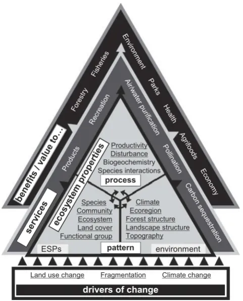
Assessments of ESs might focus on either the ESs themselves or on the key ecosystem properties that influence ESs, from which the services may be modeled or inferred. Ecosystem properties that control ES supply are themselves an interactive set of abiotic environmental conditions, organisms (labeled“ecosystem service providers”inFigure 2), anthropogenic activities (e.g., management actions), and drivers of change (Figure 2).
ES providers (Kremen2005) are not often used in ES assessments, but may be useful indicators of ES supply. The potential to use ES providers to indicate ESs derives from the considerable body of work relating biodiversity to ecosystem functioning, and the devel-oping understanding that the strongest drivers of functionality might be individual species or functional groups, rather than biodiversity per se (Hooper et al. 2005). ESs can be provided by a wide range of entities. Although plant communities are often the subject of functionality research, microbes, arthropods, and even predators are important drivers of biogeochemical cycles and ESs (de Bello et al. 2010; Kremen et al. 2007; Schmitz,
year
n
publications
1985 1990 1995 2000 2005 2010
0
200
400
600
800
1000
1200
ecosystem services mapping ecosystem services
Figure 1. The number of publications in the SCOPUS database, by year, containing the phrase
‘ecosystem services’in the title, abstract, or keywords (filled circles) and the subset of those studies containing the word‘mapping’(open circles).
Table 2. Definitions of ES terminology used in the text.
Term Definition
Benefits transfer The practice of extrapolating levels of service provisioning (per unit area) measured for a mapped class in one location to all occurrences of that class in a study extent, which may differ from that of the original measurement.
Ecological processes Fluxes of materials, energy, and organisms within ecosystems and the biotic and abiotic interactions that drive them. As with Wallace (2007), we consider ecological (ecosystem) processes to be synonymous with ecosystem functions.
Examples: photosynthesis, evapotranspiration, net primary productivity, predation.
Ecological production functions
A formula used to estimate the level of service provisioning at a particular location given the biotic and abiotic characteristics of that site. Ecological production functions may be empirical (e.g., regression) models, ecological process models, ora priorirule-based models of ES supply.
Examples: the RUSLE, which models erosion as a function of rainfall, soil characteristics, topography, and vegetation cover, is often used as an ecological production function for the ESs erosion control and water quality.
Ecosystem properties The term“ecosystem properties”collectively refers to the pattern and process of an ecological system. Thus, ecosystem properties span the abiotic environmental conditions of an ecosystem, the composition (i.e., the ES providers present) and spatial structure of an ecosystem, and the ecological processes that occur within the ecosystem (as a result of its biotic and abiotic pattern).
ESs “The benefits people obtain from ecosystems”(MEA2005). ESs can be material goods that contribute to economic livelihoods or intangible benefits that improve human health and well-being. ESs are provided by both natural and managed systems.
Examples: clean air, clean water, food, fiber, sense of place
ES ES providers The biological entities that produce a particular ES. ES providers can be identified across levels of organization (genotype, population, species, community, ecosystem) and types of organism (plants, animals, microorganisms).
Examples: carbon sequestration is often provided by forest tree
communities; nontimber forest products are provided by the particular forest species harvested by local peoples.
Functional groups Categorization of organisms (typically species) according to the ecological processes they perform or key traits that influence ecological processes. Functional group classifications can be highly variable and are often process-dependent. Functional groups can be delineated along metabolic strategies, feeding modes, physiognomy, life span, among others.
Examples: plant functional groups in a savanna system might include trees, C3 grasses, C4 grasses, broadleaved herbs, and N-fixers. Functional traits Functional traits are conceptually similar to functional groups, but are
quantitative measurements of specific attributes relevant to ecological processes rather than categorical groupings.
Examples: vegetation height, evapotranspiration rate, root depth, photosynthetic capacity, phenology.
Hawlena, and Trussell2010). Similarly, ES providers are not restricted to a particular level of organization (Luck et al.2009).
A potential disadvantage of using ES providers as indicators of services is that the functional form of the relationship between ES providers and ESs is unknown; ES provider abundance may not reflect the level of ES provisioning (e.g., Ricketts et al.
2004). In addition, specific ES providers (e.g., individual species) might be narrowly distributed and scale poorly to broad assessments (Orians and Policansky 2009). The overly specific nature of individual ES providers can be overcome by focusing not on individual components of biodiversity, but on the attributes that make them effective ES providers. For example, while particular plant species may be associated with soil stabilization, it is their root architectural traits, not their identities, that make them effective providers of this service. A focus on the distribution of the trait (dense, fibrous root systems) will increase the generality of spatial models of the service (soil stabiliza-tion) and their robustness outside the distribution of individual species. De Bello et al. (2010) provide a comprehensive review of the linkages between functional traits and ESs.
Figure 2. Conceptual diagram exploring the links between natural and anthropogenic alterations to ecological systems, ecosystem pattern (both abiotic environmental characteristics and biotic com-position of ES providers (ES providers)), ecological processes, ESs, and sectoral benefits, including several examples within each category. Properties that are underlined can be directly observed with Earth Observation data, and then used to model the remaining properties, services, and benefits. Biodiversity fits ambiguously within this framework. It is an emergent property of ecological communities or could (and often is) equally well be considered as an ESP or an ES itself.
By focusing on functional characteristics through which organisms mediate ES supply, trait-based assessments can provide more mechanistic links of ES providers to ESs. In this vein, and at a yet higher level of abstraction from ES providers, ESs may be indicated by the ecological processes (which we use synonymously with ecological functions;Table 2) that control them. Several authors have gone through extensive exercises in identifying relation-ships between ecological processes and ESs (e.g., Kienast et al.2009; Maynard, James, and Davidson2010; van Oudenhoven et al.2012). For example, the ES of climate regulation, through carbon sequestration and storage, has links to the biogeochemical processes of the carbon cycle, including carbon uptake by plants through photosynthesis. Primary production is associated with carbon sequestration and a range of provisioning services, such as agricultural production and timber yield. Many of the supporting services (i.e., services that are required for the effective provisioning of other services) identified by the Millennium Assessment’s classification of ESs (MEA2005) are ecological processes.
2.2. Anthropogenic demand for ESs
Ecosystem properties alone provide an incomplete perspective of ESs, which should be represented by both supply and demand. ESs exist at the interface of ecological and social systems (Figure 2), and thus depend on how they are perceived and used by human communities. However, to date, most spatial assessments primarily map the supply of ESs. While ESs cannot exist in isolation from people (Cowling et al. 2008; Tallis and Polasky2009,2011), it may be advantageous to model the supply of ESs independently from demand, prior to integrating these parallel spatial assessments for planning applica-tions. Demand can decouple ecological value and the effective production of ESs from economic value, obscuring mechanistic relationships and complicating management. For example, demand for urban recreation opportunities is often driven by the size of the nearby population, not by the quality of the service provided by a site (Holland, Eigenbrod, Armsworth, Anderson, Thomas, Heinemeyer et al.2011; Vejre, Jensen, and Thorsen2010). Likewise, in a Global prioritization for restoration of ESs, Luck, Chan, and Fay (2009) targeted areas with the greatest demand, but it is not clear that the chosen services can be supplied by the identified areas, especially given the long time frames and uncertain outcomes of ES restoration (Brauman et al.2007). Simple assessments of supply vs. demand may be based on patterns of spatial overlap (e.g., Burkhard et al. 2012; Nedkov and Burkhard 2012). However, ES supply and demand need not colocate, depending on the type of service and mode of delivery (Fisher, Turner, and Morling
2009). Such complexities are not often addressed (but see the ARIES (Artificial Intelligence for Ecosystem Services) toolkit, which couples independent models of ES supply and demand with novel models of the spatial flows of ESs from ecosystems to users [Bagstad et al.2011; Villa et al. 2011]).
3. Methods used to map ESs
Various strategies exist to map ESs that range in their data requirements and mechanistic complexity (Martínez-Harms and Balvanera2012). In the online supporting materials, we group ES mapping methods into five general strategies. Our categorization follows Willemen et al. (2008) and Eigenbrod et al. (2010a), who identify three basic methods of mapping ESs and ecosystem properties: (1) At the most data-intensive end, direct mapping with survey and census approaches provides complete spatial information of the distribution of a service. When spatially synoptic ES data do not exist, ESs can be
modeled across a study area using spatial socioecological data layers, and (2) empirical models of ESs developed from point-based measurements of services, or (3) if no ES data exist,a priori rule-based models. To these, we add two commonly applied methods to proxy the distribution of ESs with existing spatial data products: (4) extrapolation, and (5) data integration. With the extrapolation method, categorical landscape features (often land-cover classes) are parameterized for their level of ES supply based on aspatial summary values. Data integration studies synthesize multiple preexisting spatial products to generate ES maps, often with rule-based approaches. There are some ambiguities in these class definitions, and hybrid methods are possible. However, these five strategies loosely fit into the two broad conceptual approaches described in the following subsec-tions: benefits transfer of aspatial estimates of ES supply, and production function models, which quantify estimated mechanisms of ES supply and use.
3.1. Benefits transfer
Benefits transfer is the technique of mapping ES supply across a site using aspatial estimates of ES values derived either within the study area or, more typically, elsewhere. Values are spatialized by linking attributes to mapped landscape units (typically land use/land cover; LULC). Benefits transfer encompasses both the extrapolation and rule-based approaches described above, depending on whether the service values applied are continuous or categorical, respectively. Historically, economic values of ESs published in primary valua-tion studies were used. For example, Sutton and Costanza (2002) estimated the economic value of wetlands to be $14,785/ha and assigned this value to each hectare of wetland in an LULC map; this process was repeated for the remaining LULC classes to produce a map of ES values. Benefits transfers of dollar values are still pursued, but the transfer of biophysical measures of ESs or rankings of perceived ES capacity are also widespread. A typical example is the linking of average above-ground biomass values to LULC classes to map the distribution of the carbon storage service (e.g., Gibbs et al.2007).
Benefits transfer is a common practice (e.g., Isely et al. 2010; Sutton and Costanza
2002; Troy and Wilson2006). Advantages of benefits transfer include the transparency of the method (Koschke et al.2013) and widespread availability of the spatial indicators used (although the availability of sufficient primary economic or biophysical estimates is often limiting (Bagstad et al. (2012)). Benefits transfer will continue to be a valuable first-cut approach to ES mapping (Burkhard et al. 2012) due to limitations of time, data, and expertise (Bagstad et al.2012), which forestall the use of more sophisticated (and more complicated) methods. However, benefits transfer has received several critiques.
A shortcoming identified with benefits transfer is generalization error (Eigenbrod et al.
2010a; Plummer 2009). Generalization error results from the assumptions that the level and value of ES provisioning are constant within a mapped class, and that the ES estimate is representative (Eigenbrod et al.2010b). The use of categorical information to represent features that vary continuously in space (Eigenbrod et al.2010a; Houghton et al.2007) and time (Holland, Eigenbrod, Armsworth, Anderson, Thomas, Gaston et al.2011) may produce inaccurate spatial models. Additionally, benefits transfer generally assumes a linear relationship between habitat area and cumulative service provisioning despite known nonlinearities (Brander, Brouwer, and Wagtendonk2013; Koch et al. 2009) and threshold effects (Brauman et al.2007).
Another challenge to benefits transfer is that ESs and their values are context-specific (Birch et al.2010). Not only will biophysical variation between sites influence whether a service is provided and at what level, the sociocultural context of a site will determine the
use, value, and relative importance of ESs (Birch et al.2010; Cowling et al.2008; Verburg et al. 2009). Recent advances in benefits transfer (i.e., function transfer) address this context-dependence by deriving estimates from a suite of valuation studies, each char-acterized by the physical and socioeconomic environment studied. A meta-regression analysis is conducted to estimate ES values for the study area of interest, given its own particular context (e.g., Brander, Brouwer, and Wagtendonk2013; Ghermandi and Nunes
2013; Moeltner, Boyle, and Paterson 2007; Moeltner and Woodward 2009). Function transfer has been shown to reduce transfer errors relative to point-based transfer of single or averaged values (Ghermandi and Nunes2013).
Bayesian network modeling is another advanced method that is being used for benefits transfer (Bagstad et al. 2011; Grêt-Regamey et al. 2013; Haines-Young 2011). Such models partially address the nonmechanistic nature of benefits transfer by codifying the hypothesized links between indicators and ESs. Such links can be data-driven or derived from expert judgment. Importantly, Bayesian network models can also map uncertainty of the modeled service (Bagstad et al.2011; Grêt-Regamey et al.2013).
3.2. Ecological production functions
Ecological production functions are quantitative models of ESs that use measured eco-system properties. These models make greater attempts to mechanistically estimate the supply and flows of ESs (Kareiva et al.2011; Tallis and Polasky2009). For example, an ecological production function may model carbon storage not only as a function of LULC, but also of climate, soil fertility, and plant traits, recognizing that all of these factors contribute to carbon assimilation and emission. Ecological production functions can be simulation or process models (e.g., Band et al.2012; Crossman and Bryan2009; Doherty et al. 2010), empirical models (e.g., Willemen et al. 2008), or, when primary data are unavailable, logical models using a priori expert-based decision rules (e.g., Willemen et al.2008). An important class of empirical models of ES values (especially amenity and recreation values) is hedonic pricing models–regression models of property values based on the surrounding natural amenities, among other factors (Waltert and Schläpfer2010). Ecological production functions may support continuous, quantitative maps of service provisioning, which are essential to effectively evaluate multifunctionality and the inter-actions between services (Willemen et al.2010). For example, using quantitative estimates of services, Willemen et al. (2010) found that the extent of multifunctionality was low in their study landscape in the Netherlands and that individual services tended to be provided at higher levels when they occurred singly. In contrast, multifunctionality and interactions between services mapped by benefits transfer can be ambiguous because they only consider spatial overlap (Bennett, Peterson, and Gordon 2009) and do not indicate whether service interactions are synergistic, antagonistic, or neutral (Rodríguez et al.
2006). Ecological production functions are generally expected to be improvements over benefits transfer (Maes et al. 2012; Tallis and Polasky 2009; and demonstrated by Willemen et al. 2008). However, like all models, their quality will depend on the assumptions made and the data they are parameterized with.
4. Data for ES assessments
To date, ES mapping efforts have largely relied on existing data products (Table 3) developed for other purposes (Layke 2009), which has limited the set of services that can be mapped (Holland, Eigenbrod, Armsworth, Anderson, Thomas, Heinemeyer et al.
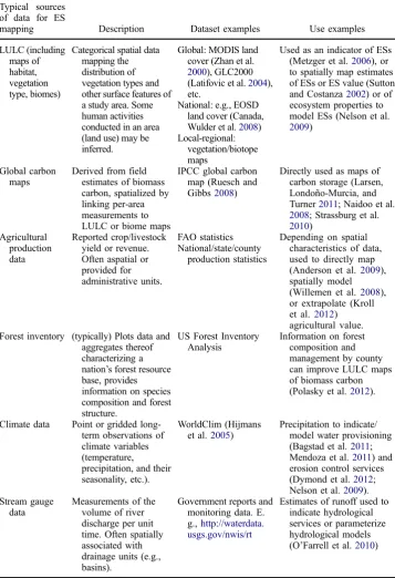
Table 3. Common sources of data used in ES mapping efforts, along with examples of datasets and their use (synthesized from online supporting materials).
Typical sources of data for ES
mapping Description Dataset examples Use examples
LULC (including maps of habitat, vegetation type, biomes)
Categorical spatial data mapping the distribution of vegetation types and other surface features of a study area. Some human activities conducted in an area (land use) may be inferred.
Global: MODIS land cover (Zhan et al.
2000), GLC2000 (Latifovic et al.2004), etc.
National: e.g., EOSD land cover (Canada, Wulder et al.2008) Local-regional:
vegetation/biotope maps
Used as an indicator of ESs (Metzger et al.2006), or to spatially map estimates of ESs or ES value (Sutton and Costanza2002) or of ecosystem properties to model ESs (Nelson et al.
2009)
Global carbon maps
Derived from field estimates of biomass carbon, spatialized by linking per-area measurements to LULC or biome maps
IPCC global carbon map (Ruesch and Gibbs2008)
Directly used as maps of carbon storage (Larsen, Londoño-Murcia, and Turner2011; Naidoo et al.
2008; Strassburg et al.
2010) Agricultural
production data
Reported crop/livestock yield or revenue. Often aspatial or provided for administrative units.
FAO statistics National/state/county
production statistics
Depending on spatial characteristics of data, used to directly map (Anderson et al. 2009), spatially model (Willemen et al. 2008), or extrapolate (Kroll et al. 2012) agricultural value. Forest inventory (typically) Plots data and
aggregates thereof characterizing a nation’s forest resource base, provides information on species composition and forest structure.
US Forest Inventory Analysis
Information on forest composition and management by county can improve LULC maps of biomass carbon (Polasky et al.2012).
Climate data Point or gridded long-term observations of climate variables (temperature, precipitation, and their seasonality, etc.).
WorldClim (Hijmans et al.2005)
Precipitation to indicate/ model water provisioning (Bagstad et al.2011; Mendoza et al.2011) and erosion control services (Dymond et al.2012; Nelson et al.2009). Stream gauge
data
Measurements of the volume of river discharge per unit time. Often spatially associated with drainage units (e.g., basins).
Government reports and monitoring data. E. g.,http://waterdata. usgs.gov/nwis/rt
Estimates of runoff used to indicate hydrological services or parameterize hydrological models (O’Farrell et al.2010)
(continued)
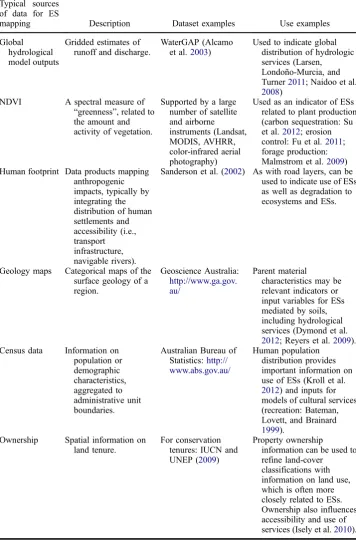
Table 3. (Continued).
Typical sources of data for ES
mapping Description Dataset examples Use examples
Soil surveys Categorical spatial data mapping the distribution of soil types, may be linked with data on chemical and physical
properties per soil type.
SSURGO database.
http://websoilsurvey. nrcs.usda.gov/
Soil maps/properties used to parameterize erosion control and hydrological services (Guo, Xiao, and Li
2000; Nelson et al.2009). Soil fertility used to indicate/model agricultural production (Lautenbach et al.2011).
Digital elevation models
Gridded elevation data, may be used to derive topographic products (e.g., slope, presence of mountains).
SRTM (Rabus et al.
2003)
Widely used to model water flows for hydrologic services (Nelson et al.
2009; Fohrer, Haverkamp, and Frede2005), erosion susceptibility (Band et al.
2012), and viewsheds for aesthetic services (Grêt-Regamey, Bishop, and Bebi2007).
Forest growth models
Statistical or process models of biomass as a function of forest age, potentially including
environmental drivers such as climate or soil data.
See references of applications to ESs.
Used to map forest services, such as timber or carbon sequestration (Bateman and Lovett2000; Bateman
2009), or to develop aspatial estimates of forest services to link with LULC data (Jenkins et al.
2010). Permit and
concessions data
Agreements for resource use, may include spatial location and quantitative allowances of use.
Mexican Public Register of Water Rights
Water extraction permits used to quantify water provisioning service (Díaz-Caravantes and Scott2010; Willemen et al.2008).
Road layers Digitized road networks Statistics Canada (2008) Road Network
Roads used to indicate access/ use of a service (e.g., recreation: Bateman, Lovett, and Brainard1999; flood protection: Nedkov and Burkhard2012), as well as potential environmental degradation reducing service provisioning (e.g., scenic views: Bagstad et al.
2012; recreation: Lautenbach et al.2011). Waterbodies Location of surface
water, including lakes, rivers, and streams
National Hydro Network:http:// geobase.ca/
Used to inform water and water-constituent routing in hydrologic service models (Bagstad et al.
2011).
(continued)
Table 3. (Continued).
Typical sources of data for ES
mapping Description Dataset examples Use examples
Global hydrological model outputs
Gridded estimates of runoff and discharge.
WaterGAP (Alcamo et al.2003)
Used to indicate global distribution of hydrologic services (Larsen, Londoño-Murcia, and Turner2011; Naidoo et al.
2008) NDVI A spectral measure of
“greenness”, related to the amount and activity of vegetation.
Supported by a large number of satellite and airborne instruments (Landsat, MODIS, AVHRR, color-infrared aerial photography)
Used as an indicator of ESs related to plant production (carbon sequestration: Su et al.2012; erosion control: Fu et al.2011; forage production: Malmstrom et al.2009) Human footprint Data products mapping
anthropogenic impacts, typically by integrating the distribution of human settlements and accessibility (i.e., transport infrastructure, navigable rivers).
Sanderson et al. (2002) As with road layers, can be used to indicate use of ESs as well as degradation to ecosystems and ESs.
Geology maps Categorical maps of the surface geology of a region.
Geoscience Australia:
http://www.ga.gov. au/
Parent material
characteristics may be relevant indicators or input variables for ESs mediated by soils, including hydrological services (Dymond et al.
2012; Reyers et al.2009). Census data Information on
population or demographic characteristics, aggregated to administrative unit boundaries.
Australian Bureau of Statistics:http:// www.abs.gov.au/
Human population distribution provides important information on use of ESs (Kroll et al.
2012) and inputs for models of cultural services (recreation: Bateman, Lovett, and Brainard
1999). Ownership Spatial information on
land tenure.
For conservation tenures: IUCN and UNEP (2009)
Property ownership information can be used to refine land-cover
classifications with information on land use, which is often more closely related to ESs. Ownership also influences accessibility and use of services (Isely et al.2010).
(continued)
2011; Naidoo et al.2008). Products may be aspatial (e.g., production statistics) and often rely on government-maintained monitoring infrastructure (e.g., runoff and baseflow data) or official permit records, which may not be available in many regions, or represent the true spatial distribution or level of sustainable service provisioning. In many cases, translating available data into estimates of ESs or ES drivers requires assumptions that detract from even those studies with a firm mechanistic underpinning. Most ES manage-ment and mapping relies on generic and/or untested assumptions (Carpenter et al.2009; de Groot et al.2010), and the indicators developed are largely hypotheses of relationships between the biophysical data in hand and the ES of interest (Haines-Young, Potschin, and Kienast2012). In addition, the data products used may have questionable accuracy at the regions or scales they are applied (Davies et al.2011; di Sabatino et al.2013; Fisher et al.
2011; van Jaarsveld et al. 2005).
4.1. Aspatial data
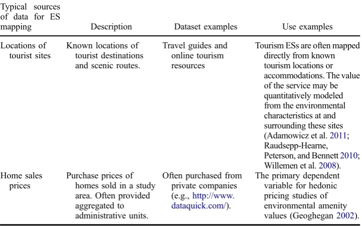
Aspatial data (or data that are effectively aspatial because they are provided at a much different scale than the ES mapping units) are used in both benefits transfer and ecological production function models of ESs to provide estimates of ES supply or biophysical variables that are linked to spatial indicators through extrapolation. For example, the InVEST models (Kareiva et al.2011) parameterize each land-cover class with estimates of the following biophysical variables: evapotranspiration, hydrologic conductivity, phos-phorus export coefficient, phosphos-phorus filtering efficiency, roughness, plant cover, and biomass and increment (Nelson et al.2009). Soil types are often parameterized for their erodibility and carbon content, among others. A number of aspatial information types have been used, as described below. Somewhat problematically, the sources of such information used to parameterize ES models are not always documented in publications. Table 3. (Continued).
Typical sources of data for ES
mapping Description Dataset examples Use examples
Locations of tourist sites
Known locations of tourist destinations and scenic routes.
Travel guides and online tourism resources
Tourism ESs are often mapped directly from known tourism locations or accommodations. The value of the service may be quantitatively modeled from the environmental characteristics at and surrounding these sites (Adamowicz et al.2011; Raudsepp-Hearne, Peterson, and Bennett2010; Willemen et al.2008). Home sales
prices
Purchase prices of homes sold in a study area. Often provided aggregated to administrative units.
Often purchased from private companies (e.g.,http://www. dataquick.com/).
The primary dependent variable for hedonic pricing studies of environmental amenity values (Geoghegan2002).
4.1.1. Expert judgment
Expert opinion is widely used to associate ES capacity with spatial data layers, particu-larly when data, resources, or technical expertise are limiting. Expert opinion has linked categorical indicators to ESs with binary relationships (a class does or does not provide a service; e.g., Kienast et al. 2009) or ordinal rankings of classes by their capacity for service provisioning (e.g., Burkhard et al.2012; Koschke et al. 2012) via lookup tables (e.g., Burkhard et al.2012; Kienast et al.2009; Koschke et al.2012) or Bayesian network models (e.g., Bagstad et al.2011; Grêt-Regamey et al.2013), among other approaches. Expert judgment can also modify general patterns to local conditions (e.g., Haines-Young, Potschin, and Kienast2012; Scolozzi, Morri, and Santolini2012).
Expert parameterizations allow for flexible, rapid ES assessments, but might be best taken as working models. For example, mistaken perceptions of the drivers of a given system can lead to incorrect model parameterizations (as described in Bruijnzeel (2004)). In addition, experts’ opinions will depend on their backgrounds and values. Different stakeholder or expert groups can weight factors differently, set different thresholds of service supply, or disagree on the relationships between indicators and services (Bryan et al. 2011; Gos and Lavorel 2012; Nahuelhual et al. 2013; Plieninger et al. 2013; Scolozzi, Morri, and Santolini2012; Sherrouse, Clement, and Semmens2011).
4.1.2. Production statistics
Production statistics reported by government agencies and international organizations are a valuable source of quantitative ES values and categorical (e.g., crop type) information, especially for the provisioning services. Such statistics may be in economic terms or physical yield units. Although such data are, to some extent, spatial, they are often more coarsely aggregated (e.g., to administrative boundaries) than the analysis units of ES assessments. Per-area values are often derived and attributed to the relevant provisioning LULC categories within each reporting unit (e.g., Eigenbrod et al.2009; Kroll et al.2012; Raudsepp-Hearne, Peterson, and Bennett 2010). It is important to note that production statistics inform on current levels of ES use, rather than potential or sustainable capacities (Maes et al.2012).
4.1.3. Empirical data
ES or parameter values may be directly estimated, usually with point-based measurements or their averages (rather than areal aggregates, like production statistic data). The sources of empirical data are broad. They can be measured specifically for ES assessment (e.g., Davies et al. 2011); derived from archived data, such as forest inventories (e.g., Birch et al. 2010; Jenkins et al.2010); or extracted from published values, such as from the primary valuation literature (e.g., Eade and Moran1996).
4.1.4. Model outputs
Finally, models can be sources of ES values or production function parameters. For example, timber yield and carbon sequestration can be estimated from forest growth models and extrapolated over forested land cover (e.g., Vicente et al. 2013; Jenkins et al. 2010). Nedkov and Burkhard (2012) present a novel approach to estimate flood
control capacity of land-cover classes and soil types based on their overlap with spatial hydrological model outputs.
4.2. Spatial data
Spatial data are necessary to map the distribution of ESs. A variety of spatial information, representing different aspects of socioecological systems, is in use. This spatial informa-tion can indicate ESs directly or be integrated with other spatial data layers using rule-based, empirical, or process models.
4.2.1. Land use/land cover
By far, the most widely used type of information in ES assessments is LULC maps (Seppelt et al.2011). LULC products are frequently used in benefits transfer to spatialize per-area estimates of ES supply. They are also often relied on to produce the spatially distributed biophysical parameter values needed for production function models (e.g., many of the InVEST models, Kareiva et al.2011).
The ubiquity of LULC datasets in ES assessments is not difficult to understand. Land-use change is a major proximate driver of ES loss (Foley et al.2005; MEA2005). LULC products provide abundant, detailed information relevant to many environmental patterns and processes. They have widespread availability at a range of scales, all over the world, and their information content is easy to understand and apply. Furthermore, they can be used to estimate changes in ES provisioning from observed LULC changes (e.g., Carreño, Frank, and Viglizzo2012; Lautenbach et al.2011; Leh et al.2013; Li et al.2010) and by relatively seamless linkages with future land-use scenarios (e.g., Kienast et al. 2009; Nelson et al.2009). However, LULC products are not a panacea to spatial data needs, and it is important to consider their effectiveness for a given application.
Remotely sensed data, especially coarse-scale LULC products, primarily represent land cover. However, land use and management actions are better indicators of ESs than land cover (Ericksen et al. 2012; Koschke et al. 2013; van Oudenhoven et al. 2012). Substantial changes in land use, such as agricultural intensification or pasture abandon-ment, may have profound impacts on ESs, but be undetected in coarse-scale remotely sensed land-cover products (Verburg et al. 2009). For example, in the former German Democratic Republic, large demographic changes and the introduction of alternative land uses (such as wind farms) led to noticeable changes in ES supply and use, despite relatively little change in land cover (Burkhard et al. 2012; Kroll et al. 2012). Supplemental data (such as cropping system, land ownership, production statistics, etc.) may augment land-cover data with greater details on land use, improving ES assessments (Ericksen et al. 2012; Lesschen et al. 2007; Koschke et al.2013; Mehaffey et al.2011; Swallow et al.2009).
In addition, land cover may not be a reliable indicator of the ecosystem properties that influence ESs, and consequently may poorly represent the services themselves. For example, shoreline protection is often proxied by the areal coverage of coral reefs. However, wave attenuation is more closely linked to the vertical complexity of coral architecture, which is related to coral cover only weakly, at best (Alvarez-Filip et al.
2011). Likewise, associations of species composition with land cover are relatively weak (Andrew, Wulder, and Coops 2011). Nevertheless, Dahlin, Asner, and Field (2013) observed that, although within-class variation was high, the spatial distribution of plant functional traits was best explained by vegetation type. To date, the ability of LULC to
indicate ESs has rarely been tested (de Groot et al.2010; Martínez-Harms and Balvanera
2012; but see Raudsepp-Hearne, Peterson, and Bennett2010).
Finally, the use of categorical LULC information to parameterize ES assessments is a source of the generalization error associated with benefits transfer (see Section 3.1). LULC classes are not internally homogenous, instead exhibiting variation based upon the raster-based organization of features that are continuous on the landscape. Additionally, the spatial resolution of the imagery dictates the level of detail that is captured and can be reasonably used as category labels. The elements that vary con-tinuously, that will have an impact upon the range of conditions related in a given pixel, include species composition, the age, structure, and condition of the plant communities, and local variation in conditions related to land use or abiotic conditions, among other factors. Thus, overly coarse classes may obscure variation that is relevant to ESs (Koschke et al.2013; Vihervaara et al.2012). Hedonic pricing studies (that is, studies to determine what factors add value to properties, such as an ocean view, or access to natural areas, see
Section 3.2) have shown that the type of open space and forested land cover present has significant effects on amenity values (e.g., Cho, Poudyal, and Roberts 2008). The assumption of homogeneity within a class is sometimes addressed by partitioning the study region into a larger number of very fine classes along such factors as ecosystem age and condition (e.g., Nelson et al. 2009). This strategy is problematic, however, as classification accuracy generally decreases sharply with increasing level of thematic detail (Fassnacht, Cohen, and Spies 2006; Remmel et al. 2005). Notwithstanding the need for accurate model inputs, Skidmore et al. (2011) note that error characteristics of input products are rarely considered in ES studies. Another challenge of high thematic resolu-tion LULC classificaresolu-tions in the ES mapping context is that the greater number of classes to be parameterized may result in unrealistic data requirements (Bagstad et al. 2012; Jackson et al.2013; Nemec and Raudsepp-Hearne2013).
4.2.2. Physical data describing the environment
Many ES models make use of spatial datasets representing various features of the earth’s surface (Table 3). These data products are generally quite well established, and many are available in physical units.
4.2.2.1. Topography.Elevation and topographic variables derived from digital elevation models (DEMs) feature prominently in models of hydrological services. DEMs are used to determine flow paths and hydraulic connectivity to assess freshwater supply, flow regulation (e.g., Bagstad et al.2011), geomorphology (Blanchard, Rogan, and Woodcock
2010), and water purification (e.g., Conte et al.2011). Slope surfaces derived from DEMs are frequently used to model erosion control and sediment regulation. These ES models range in sophistication from rule-based approaches (e.g., areas of steep slope as a surrogate for sediment sources: Lautenbach et al.2011) to the revised universal soil loss equation (RUSLE; one of the most common means to map these services; e.g., Lautenbach et al. 2011) and process models (e.g., Band et al. 2012; Vigerstol and Aukema2011).
Models of tourism and aesthetic values also tend to enlist topographic surfaces, specifically, viewshed models. A viewshed is the total extent visible from a vantage point, and is determined by the lay of the land and the presence of obstructions (trees or buildings). The latter are generally ignored as such data (from a digital surface model as opposed to a DEM) are not typically available. The magnitude of the viewshed (Sander
and Haight 2012) and its components (i.e., pleasing views or ‘visual blights’; Grêt-Regamey, Bishop, and Bebi2007; Sander and Haight 2012; Bagstad et al. 2012) deter-mine the aesthetic quality of the vista.
Topography provides inputs to empirical models of a range of other services (e.g., agricultural and timber production: Bateman et al. 1999) and has been used in expert systems to refine estimates of agricultural productivity (e.g., using slope to define marginal lands with low production, Jackson et al.2013) and greenhouse gas mitigation (Jenkins et al.2010), among other applications. Bathymetry layers are a major source of information for ES assessments of aquatic and marine systems, for which they are used as is (e.g., in models of coastal flood protection (Liquete et al. 2013), or wave energy generation (Kim et al.2012)), or to generate habitat maps (e.g., Allan et al. 2013).
4.2.2.2. Soil maps.Soils are essential components of the earth system and play important direct and indirect roles in the provisioning of many ESs (Haygarth and Ritz 2009; Robinson et al. 2013), including agricultural and timber production, and hydrological and carbon services. Soil properties are frequently included in biophysical (Crossman and Bryan2009; Vigerstol and Aukema2011) and empirical (e.g., Lavorel et al.2011) models of ESs or ES providers. Soil type has also been used for benefits transfer (e.g., of carbon storage: Egoh et al. 2011; of agricultural production, especially when intersected with agricultural land cover: Chan et al.2006; Lautenbach et al.2011). Categorical soil maps are the usual source of spatial soil data for ES assessments, although these may be attributed with quantitative characteristics of each soil type. In much of the world, spatial soil data products are inadequate (Sanchez et al. 2009) or unavailable (Rossiter 2004). Soil maps are typically generalized polygon-based representations. Outside of agricultural regions, soil maps are often developed through an interpretation-based approach, where soil attributes are assigned based upon knowledge of geological conditions and expected associations with the vegetation (often trees) present. While reasonable for providing for inferences or trends over larger areas (Maynard et al.2014), users should be circumspect in developing ES models that require detailed, spatially explicit, soil data.
4.2.2.3. Climate data.Climate and weather are important drivers of ESs and, as such, are often considered in ES assessments. Climate layers are required inputs for process models of carbon sequestration and agricultural or forest production (e.g., Doherty et al. 2010; Schulp et al.2012) and for many models of hydrological services (e.g., Dymond et al.
2012). Climate may also influence tourism potential (Ghermandi and Nunes 2013). Sources of gridded climate data include interpolated observations from weather stations (e.g., Hijmans et al. 2005) and global and regional climate model outputs (e.g., http:// www.ipcc-data.org/). ES models that directly incorporate climatic drivers can be used to evaluate climate change scenarios (e.g., Bangash et al.2013; Schröter et al. 2005). For example, Doherty et al. (2010) forecasted that, in their study area, land cover will remain unchanged under future climate, but large changes to carbon sequestration will occur due to changes within the dominant cover type. The widespread availability of gridded climate data has prompted widespread use, but with little discussion of the uncertainties contained within such datasets, especially at the fine spatial scales relevant to ES planning and monitoring. Climate surfaces are typically developed from relatively coarse scale esti-mates, either potentially sparse station measurements or general circulation models. Many of the interpolation and downscaling methods employed to produce the final data products do not account for climate drivers that operate on fine scales (Daly 2006), introducing spatial and temporal inaccuracies in the resulting climate surfaces (Hofstra, New, and
McSweeney 2010) and the ecological processes and ESs modeled from them (e.g., Bárdossy and Das2008).
4.2.2.4. Productivity. Productivity is understood to have widespread relevance to ESs (Balvanera et al. 2006; Boumans et al. 2002; DeFries, Foley, and Asner 2004). Productivity is directly related to provisioning and carbon-related services. Modeled (e.g., Doherty et al.2010; Schröter et al.2005) and remotely sensed (Raudsepp-Hearne, Peterson, and Bennett2010; Su et al.2012; Vicente et al.2013) estimates of productivity and biomass have been used to assess carbon services, although the latter source of productivity information has been used surprisingly infrequently. Sutton and Costanza (2002) suggest that primary productivity may be an effective surrogate of total ES value. Building on this hypothesis, Carreño, Frank, and Viglizzo (2012) incorporated productiv-ity into rule-based models of most services assessed (including soil protection, production, water purification, water provisioning, and disturbance regulation). However, Egoh et al. (2008) found generally weak relationships between productivity and ES supply. The relationships between productivity and ESs merit further investigation to demonstrate their generality, and can be well supported by remotely sensed estimates of vegetation activity (Andrew, Wulder, and Nelson2014).
4.2.2.5. Hydrological data. Some studies use existing spatial datasets of hydrological parameters, such as runoff, baseflow, groundwater recharge, or water quality, to indicate hydrological services directly (e.g., Larsen, Londoño-Murcia, and Turner2011; O’Farrell et al.2010). These datasets may be derived from observations (e.g., gauging stations) or from model outputs. Although some are published data products, others are described in the gray literature and it can be difficult to ascertain how they were created and using what sources of information. These datasets are available variously in gridded format, asso-ciated with watershed polygons, or as point measurements.
4.2.3. Descriptors of the socioeconomic context
Thus far, the focus has been on data sources used to map the supply of ESs. Demand for ESs can be assessed by characterizing the population of likely users and accessibility of a service. The most obvious proxy of demand is a map of the human population distribution (e.g., Kroll et al.2012). Although note that ES use can be distant from its supply (Fisher, Turner, and Morling2009) and that users from different spatial extents can have different ES values and priorities (Hein et al.2006). Population characteristics can have important effects on the spatial distribution of demand. For example, poverty is believed to increase ES demand (Luck, Chan, and Fay 2009), but the monetary value of ESs is greater in wealthier areas (e.g., Ghermandi and Nunes2013). Ethnic, demographic, and stakeholder group membership influences the distribution and estimates of ES values (Saphores and Li
2012; Sherrouse, Clement, and Semmens2011; Waltert and Schläpfer2010), as does the institutional and market context (Leefers and Potter-Witter2006).
Population and economic data may not exist at the appropriate spatial resolution for ES assessments. An interesting means to proxy the distribution of human populations and economic activity is by the amount of artificial light detected in nighttime satellite images (the Defense Meteorological Satellite Program nighttime lights dataset: Elvidge et al.
1997). Such information has been related to ES values by Sutton and Costanza (2002) and Forbes (2013). Alternatively, the distribution of human infrastructure, which may be extracted from LULC products or transportation data layers, can proxy ES demand. For
example, it is generally desired that buildings and roads be protected from floods, avalanches, and other disturbances; thus, their presence indicates demand for distur-bance-regulating services (e.g., Grêt-Regamey et al. 2013; Liquete et al. 2013; Nedkov and Burkhard2012). Roads also determine access to regions and ESs, with concomitant effects on the use and value of services. Road networks have been included in a number of ES models (e.g., recreation: Lautenbach et al. 2011; forest products: Orsi, Church, and Geneletti2011). Roads and paths may be required components of the service itself, as in the case of some recreation activities (e.g., Gulickx et al.2013; Haines-Young et al.2006; Willemen et al.2008). More recently, spatial maps of access to computing resources, such as maps of internet protocol (IP) addresses,‘Facebook’friend links, and other geotagged social media data, offer new tantalizing opportunities (e.g., Richards and Friess 2015). Another aspect of the social context that influences ESs is ownership. Land tenure affects the quantity and value of services provided by an area by determining access (Isely et al.
2010) and influencing the perceived stability and quality of the service (Geoghegan2002; Irwin2002).
5. Discussion
The current paradigms for mapping ES provisioning – via ecological production func-tions, ES providers, or functional traits – provide a strong scientific framework. Challenges remain in the implementation of ES mapping efforts due to limitations of the available data products. Diverse approaches have been developed to utilize existing information sources in ES assessments. In many cases, the same ES has been modeled in a variety of ways. For example, the regulating service of carbon sequestration has been mapped using various process model outputs (biomass increment: Crossman and Bryan
2009; net carbon exchange: Naidoo et al. 2008), several remotely sensed indicators (NDVI: Su et al. 2012; MODIS Net Primary Productivity (NPP): Raudsepp-Hearne, Peterson, and Bennett 2010), and accounting models parameterized by LULC (e.g., Nelson et al. 2009). Numerous other examples, for other services, can be found in the online supporting information. Some authors argue that such a diversity of approaches is a weakness and standardized ES assessments should be developed (Crossman, Burkhard, and Nedkov 2012; Maes et al. 2012). Others note that a diversity of approaches will support innovation (Seppelt et al. 2012), and that the heterogeneity of socioecological systems will demand ES assessments tailored to particular contexts, preventing the successful application of standardized procedures (Gulickx et al.2013).
The main argument for standardized mapping and modeling practices is that different methods yield discrepancies in the spatial patterns of mapped ESs (Eigenbrod et al.
2010a), the locations and levels of ES overlap (Eigenbrod et al. 2010a) or tradeoffs (Nelson et al. 2009), and estimates of the change in ES supply over time (Lautenbach et al.2011; Lavorel et al.2011). However, direct comparisons of different ES assessment strategies are rare as most efforts typically only apply one set of methods. Further, the outputs of different approaches may not be readily comparable, as different spatial analysis units or service indicators are often used (Bagstad et al. 2012; Kienast et al.
2009; Nahlik et al. 2012). More comparative applications of different ES mapping techniques are needed (Vigerstol and Aukema2011).
Discrepancies between ES assessments call the utility of the mapped ES products into doubt, as it is unclear which representations are more accurate. The real problem here is not that different spatial portrayals exist, but that a concrete means to evaluate and rank them is currently missing. Although there exist common practices and guidelines for
assessing the accuracy of spatial data products (e.g., cover: Foody 2002; Stehman and Foody 2009; change: Olofsson et al. 2014), most ES mapping efforts lack validation efforts (Seppelt et al.2011).
A further limitation is the varying suitability of existing spatial data for the ES assessments to which they are applied. There appears to be a frequent tradeoff between quantitative data that are directly related to ESs or their underlying ecosystem properties and indirect proxies that are provided by readily available, spatially extensive data products. (We argue elsewhere that this tradeoff need not be the case in all situations, and a number of direct estimates of ecosystem properties that are directly relevant to ESs may be supported by contemporary remote sensing: Andrew, Wulder, and Nelson [2014].) In accord with previous reviews (Martínez-Harms and Balvanera 2012; Seppelt et al.
2011), we find that benefits transfer and expert-driven rule-based overlays are widespread strategies to reconcile this data gap and map the economic and biophysical values of ESs. Such assessments are appealing in many circumstances, because they are not onerously burdened by the data to be gathered or technical skills needed to apply them. However, they necessarily provide indirect, generalized surrogates reflecting hypotheses of ES supply and/or use.
Despite their prominence in ecological studies of ESs, ES providers are rarely used for ES mapping. The focus on mapping ESs, rather than their providers, may be because the dominant ES providers in a study region remain unknown, or functionality is distributed between many species and influenced by complicated interactions, making a focus on the ultimate service pragmatic (Kremen et al.2007; Luck et al.2009). It may also reflect the preference to manage for pattern rather than process (Wallace2007). However, there are a few examples of mapping services via their underlying providers, where the link between providers and services is readily apparent, as when the service is focused on particular species (e.g., game species for recreation or bushmeat provisioning). These services can be mapped using habitat suitability modeling of the target species (e.g., Naidoo and Ricketts 2006). Plant traits as ES providers have been empirically modeled across a landscape by Lavorel et al. (2011) to support the mapping of ecosystem processes and services, providing better ES models than LULC proxies alone.
There are a large number of increasingly mechanistic ES assessments that apply empirical or process models of the biophysical and social controls on the production and flows of ESs. Parameterization of these models is somewhat mixed. Well-established, spatially extensive, quantitative datasets of various abiotic ecosystem properties (espe-cially climate and topographic data) exist and are widely used. However, many other ecosystem properties, particularly those characterizing organisms and their traits that influence ES supply, as well as soil properties, are represented more indirectly via links to qualitative LULC and soil maps. Although efforts are often made to attribute mapped categories with empirical, modeled, or production statistics estimates of the relevant ESs or ecosystem properties, because of the nature of the spatial data, the resulting products are, at most, semiquantitative.
6. Conclusions
Despite the relative youth of the field, there is a large body of ES research and growing understanding of how socioecological characteristics influence the production, use, and value of ESs. Spatial assessments of the distribution of ESs, regardless of their level of mechanistic complexity, often draw on this conceptual understanding and frame their models with the established and hypothesized relationships between ecosystem properties,
ecological processes, and the ESs of interest. Unfortunately, all too often, the data that are utilized to parameterize ES models represent these properties coarsely. Without validation efforts, it may be difficult for others to accept the simplifying assumptions that were made and to operationally apply the resulting maps. We encourage increased use of spatial estimates of quantitative biophysical parameters in ES models and assessments to avoid-ance oversimplifications. Improved maps (Eigenbrod et al. 2010a), mapping techniques (Egoh et al.2007), and spatial parameterizations, as rigorously demonstrated by quanti-tative validation of the modeled ESs, can increase user confidence in the spatial products, better support decision-making, and lead to improved planning outcomes.
Acknowledgment
Three anonymous reviewers are thanked for their insightful and challenging insights.
Disclosure statement
No potential conflict of interest was reported by the authors.
Funding
This study was funded by“BioSpace: Biodiversity monitoring with Earth Observation data”through the Government Related Initiatives Program (GRIP) of the Canadian Space Agency.
Supplemental data
Supplemental data for this article can be accessedhere.
References
Adamowicz, W. L., R. Naidoo, E. Nelson, S. Polasky, and J. Zhang. 2011.“Nature-Based Tourism and Recreation.” In Natural Capital: Theory and Practice of Mapping Ecosystem Services, edited by P. Kareiva, H. Tallis, T. H. Ricketts, G. C. Daily, and S. Polasky, 188–205. Oxford: Oxford University Press.
Alcamo, J., P. Döll, T. Henrichs, F. Kaspar, B. Lehner, T. Rösch, and S. Siebert. 2003.
“Development and Testing of the Watergap 2 Global Model of Water Use and Availability.” Hydrological Sciences Journal48: 317–337. doi:10.1623/hysj.48.3.317.45290.
Allan, J. D., P. B. McIntyre, S. D. P. Smith, B. S. Halpern, G. L. Boyer, A. Buchsbaum, G. A. Burton, et al. 2013.“Joint Analysis of Stressors and Ecosystem Services to Enhance Restoration Effectiveness.” Proceedings of the National Academy of Sciences of the United States of America110: 372–377. doi:10.1073/pnas.1213841110.
Alvarez-Filip, L., I. M. Côté, J. A. Gill, A. R. Watkinson, and N. K. Dulvy. 2011.“Region-Wide Temporal and Spatial Variation in Caribbean Reef Architecture: Is Coral Cover the Whole Story?”Global Change Biology17: 2470–2477. doi:10.1111/j.1365-2486.2010.02385.x. Anderson, B. J., P. R. Armsworth, F. Eigenbrod, C. D. Thomas, S. Gillings, A. Heinemeyer, D. B.
Roy, and K. J. Gaston. 2009.“Spatial Covariance between Biodiversity and Other Ecosystem Service Priorities.” Journal of Applied Ecology 46: 888–896. doi:10.1111/ j.1365-2664.2009.01666.x.
Andrew, M. E., M. A. Wulder, and N. C. Coops. 2011.“How Do Butterflies Define Ecosystems? A Comparison of Ecological Regionalization Schemes.” Biological Conservation 144: 1409– 1418. doi:10.1016/j.biocon.2011.01.010.
Andrew, M. E., M. A. Wulder, and T. A. Nelson. 2014.“Potential Contributions of Remote Sensing to Ecosystem Service Assessments.” Progress in Physical Geography 38: 328–353. doi:10.1177/0309133314528942.
Bagstad, K. J., D. Semmens, R. Winthrop, D. Jaworski, and J. Larson. 2012.Ecosystem Services Valuation to Support Decision Making on Public Lands–A Case Study of the San Pedro River Watershed, Arizona, 93 p. US Geological Survey Scientific Investigations Report 2012–5251.
http://pubs.usgs.gov/sir/2012/5251/
Bagstad, K. J., F. Villa, G. W. Johnson, and B. Voigt. 2011. ARIES - Artificial Intelligence for Ecosystem Services: A Guide to Models and Data, Version 1.0. ARIES Report Series n.1. The ARIES Consortium.http://ariesonline.org/docs/ARIESModelingGuide1.0.pdf
Balmford, A., A. S. L. Rodrigues, M. Walpole, P. ten Brink, M. Kettunen, L. Braat, and R. de Groot. 2008. The Economics of Biodiversity and Ecosystems: Scoping the Science. Cambridge: European Commission (contract: ENV/070307/2007/486089/ETU/B2).
Balvanera, P., A. B. Pfisterer, N. Buchmann, J.-S. He, T. Nakashizuka, D. Raffaelli, and B. Schmid. 2006. “Quantifying the Evidence for Biodiversity Effects on Ecosystem Functioning and Services.”Ecology Letters9: 1146–1156. doi:10.1111/j.1461-0248.2006.00963.x.
Band, L. E., T. Hwang, T. C. Hales, J. Vose, and C. Ford. 2012. “Ecosystem Processes at the Watershed Scale: Mapping and Modeling Ecohydrological Controls of Landslides.” Geomorphology137: 159–167. doi:10.1016/j.geomorph.2011.06.025.
Bangash, R. F., A. Passuello, M. Sanchez-Canales, M. Terrado, A. López, F. J. Elorza, G. Ziv, V. Acuña, and M. Schuhmacher. 2013. “Ecosystem Services in Mediterranean River Basin: Climate Change Impact on Water Provisioning and Erosion Control.”The Science of the Total Environment458–460: 246–255. doi:10.1016/j.scitotenv.2013.04.025.
Bárdossy, A., and T. Das. 2008.“Influence of Rainfall Observation Network on Model Calibration and Application.” Hydrology and Earth System Sciences 12: 77–89. doi: 10.5194/hess-12-77-2008.
Bateman, I. J. 2009. “Bringing the Real World into Economic Analyses of Land Use Value: Incorporating Spatial Complexity.” Land Use Policy 26: S30–S42. doi:10.1016/j. landusepol.2009.09.010.
Bateman, I. J., C. Ennew, A. A. Lovett, and A. J. Rayner. 1999. “Modelling and Mapping Agricultural Output Values Using Farm Specific Details and Environmental Databases.” Journal of Agricultural Economics50: 488–511. doi:10.1111/j.1477-9552.1999.tb00895.x. Bateman, I. J., and A. A. Lovett. 2000. “Estimating and Valuing the Carbon Sequestered in
Softwood and Hardwood Trees, Timber Products and Forest Soils in Wales.” Journal of Environmental Management60: 301–323. doi:10.1006/jema.2000.0388.
Bateman, I. J., A. A. Lovett, and J. S. Brainard. 1999. “Developing a Methodology for Benefit Transfers Using Geographical Information Systems: Modelling Demand for Woodland Recreation.”Regional Studies33: 191–205. doi:10.1080/00343409950082391.
Bennett, E. M., G. D. Peterson, and L. J. Gordon. 2009. “Understanding Relationships among Multiple Ecosystem Services.” Ecology Letters 12: 1394–1404. doi: 10.1111/j.1461-0248.2009.01387.x.
Birch, J. C., A. C. Newton, C. A. Aquino, E. Cantarello, C. Echeverria, T. Kitzberger, I. Schiappacasse, and N. T. Garavito. 2010.“Cost-Effectiveness of Dryland Forest Restoration Evaluated by Spatial Analysis of Ecosystem Services.”Proceedings of the National Academy of Sciences of the United States of America107: 21925–21930. doi:10.1073/pnas.1003369107. Blanchard, S., J. Rogan, and D. Woodcock. 2010.“Geomorphic Change Analysis Using ASTER
and SRTM Digital Elevation Models in Central Massachusetts, USA.” GIScience & Remote Sensing47: 1–24. doi:10.2747/1548-1603.47.1.1.
Boumans, R., R. Costanza, J. Farley, M. A. Wilson, R. Portela, J. Rotmans, F. Villa, and M. Grasso. 2002. “Modeling the Dynamics of the Integrated Earth System and the Value of Global Ecosystem Services Using the GUMBO Model.” Ecological Economics 41: 529–560. doi:10.1016/S0921-8009(02)00098-8.
Brander, L., R. Brouwer, and A. Wagtendonk. 2013.“Economic Valuation of Regulating Services Provided by Wetlands in Agricultural Landscapes: A Meta-Analysis.”Ecological Engineering 56: 89–96. doi:10.1016/j.ecoleng.2012.12.104.
Brauman, K. A., G. C. Daily, T. K. Duarte, and H. A. Mooney. 2007.“The Nature and Value of Ecosystem Services: An Overview Highlighting Hydrologic Services.” Annual Review of Environment and Resources32: 67–98. doi:10.1146/annurev.energy.32.031306.102758. Bruijnzeel, L. A. 2004.“Hydrological Functions of Tropical Forests: Not Seeing the Soil for the
Trees?” Agriculture, Ecosystems & Environment 104: 185–228. doi:10.1016/j. agee.2004.01.015.