New Measurement Method for Spline Shaft Rolling Performance Evaluation using Laser Displacement Sensor

ORIGINAL ARTICLE

New Measurement Method for Spline

Shaft Rolling Performance Evaluation using

Laser Displacement Sensor

Hong‑Wei Li

_{, Zhi‑Qiang Liang}

_{, Jia‑Jie Pei}

_{, Li Jiao}

_{, Li‑Jing Xie}

_{and Xi‑Bin Wang}

Abstract

In order to control the quality of spline shaft in rolling process, an efficient measurement method for rolling perfor‑ mance evaluation is essential. Here, a newly developed on‑machine non‑contact measurement prototype based on laser displacement sensor and rotary encoder is proposed. The prototype is intended for the automated evaluation of the spline shaft rolling performance by measuring the dimensional change of tooth root, which is correlated with the surface residual stress and micro‑hardness. Laser displacement sensor and rotary encoder are used to record the polar radius and polar angle of each point on measuring section. Data are displayed in a polar coordinate system and fitted in a gear. Through multipoint curvature method, the roots of spline shaft are recognized automatically. Then, the dimensional change can be calculated by fitting the radius of the tooth root circle before and after rolling. Systematic error covering offset error is also analyzed and calibrated. At last, measurement test results show that the system has advantages of simple structure, high measurement precision (radius error < 0.6 μm), high measurement efficiency (measuring time < 2 s) and automatic control ability, providing a new opportunity for the efficient evaluation of vari‑ ous spline shafts in high‑precision mechanical processing.

Keywords: Laser measurement, Spline shaft, Rolling performance, Dimensional change

© The Author(s) 2018. This article is distributed under the terms of the Creative Commons Attribution 4.0 International License (http://creat iveco mmons .org/licen ses/by/4.0/), which permits unrestricted use, distribution, and reproduction in any medium, provided you give appropriate credit to the original author(s) and the source, provide a link to the Creative Commons license, and indicate if changes were made.

1 Introduction

Spline shaft is an important part of a machine to transmit power or bear torque. Its section contour is like a gear. It suffers from great loads and alternating stress during the runtime. The tooth root of the spline shaft has a risk of fracture due to fatigue stress [1–4]. Thus, it is essential to conduct a surface hardening process such as rolling after machining. In order to control the quality of product, a rolling performance evaluation becomes essential. The commonly used evaluation parameters of surface integ-rity involve the surface roughness, the surface residual stress and the micro-hardness. However, measurement of surface roughness or through-thickness residual stresses in difficult locations or complex geometries is not easy. Many measurement techniques are destructive, such as

the centre-hole drilling method, the ring core method and the block removal method. There are non-destruc-tive techniques (e.g., X-ray and neutron diffraction, opti-cal, magnetic or ultrasonic methods) [5], but they often require the off-machine measuring. Note that for the rolling process, it is an efficient alternative to conven-tional cutting processes to manufacture spline shaft as it possesses several advantages i.e. shorter process times, no material loss and no chip disposal, high surface qual-ity [6]. The residual stress is only induced by the residual strain and the residual strain appears as the dimensional change in the macroscopic view. Therefore, it is probably feasible to use the dimensional change of tooth root as an alternative evaluation parameter.

The dimensional change of the tooth root is about 20 μm after rolling. Thus, the measurement precision of the conventional mechanical measuring instrument is not enough and it is time-consuming due to the complex-ity of the spline shaft. In order to solve such problems, it is necessary to develop a new measuring system with

Open Access

*Correspondence: [email protected]

1 _{Key Laboratory of Fundamental Science for Advanced Machining,} Beijing Institute of Technology, Beijing 100081, China

high efficiency and high precision. The laser triangula-tion displacement sensor (LDS) is a common-used tool in high precision and short-distance measuring, which can measure the displacement change of an object with-out any contact. It is mainly used in automatically meas-uring the geometrical parameter such as thickness, distance, diameter, etc [7–10]. Over a period of time there were several novel measuring systems by combin-ing it with other devices, such as identification of loca-tion error of rotary axes for five-axes machine tools [11], on machine measurement of RFQS [12], automated inner dimensional measurement system for long-stepped pipes [13] and piston secondary motion measurement [14]. For spline shaft measuring system, a rotary encoder is needed to record the rotation angle. Together with the radius recorded by the laser displacement sensor, the sec-tion contour of the spline shaft is obtained by plotting each point of the measuring section in a polar coordinate system.

The section contour of the spline shaft is like a gear, but the method used in gear measurement cannot be directly applied to our system, because most of them require the workpiece to be measured off-machine [15]. Besides, for gear measurement, researchers usually care more about the tooth thickness, tooth pitch [16], tooth flank [17] and cutting error [18]. While in the spline shaft measur-ing, the position of the tooth roots and their dimensional change should be focused, which are different from the previous gear measurement.

In this paper, a newly developed on-machine non-contact measurement prototype based on laser displace-ment sensor and rotary encoder is proposed. Firstly, by using this prototype, the section contour of spline shaft is quickly measured. Then, through multipoint curvature method (MCM), the roots of spline shaft can be recog-nized automatically. At last, the dimensional change can be calculated by fitting the radius of the tooth root circle before and after rolling. The offset error and its calibra-tion method were also discussed in this paper. Measure-ment test results show that the system has advantages of simple structure, high measurement precision, high measurement efficiency and automatic control ability.

2 Principle of the Measurement

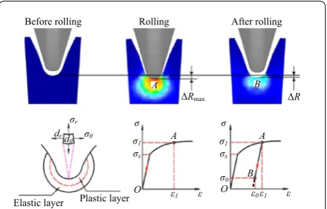
The rolling process is shown schematically in Figure 1. As can be seen in the upper part of Figure 1, when roll-ing begins, the material deforms at first elastically and then plastically, at last reaches the maximal deforma-tion ΔRmax in state A. After rolling, a certain degree of elasticity recovery occurs, thus, the final dimensional change ΔR in state B is less than its maximal value. The stress and strain analysis of the rolling process

is shown in the lower part of Figure 1. The stress and strain, denoted as σ and ε respectively, are determined from the load P and deflection δ using the original specimen cross-sectional area A0 and length L0 in ten-sile test as

when the stress σ is plotted against the strain ε, an engi-neering stress-strain curve of the material such as that shown in Figure 1 is obtained.

In the state of A, it can be seen that as strain is increased beyond the yield point, the stress deviate from its linear proportionality, and the point of depar-ture is termed as the proportional limit. This nonlinear-ity is usually associated with stress-induced “plastic” flow in the specimen. Here the material is undergoing a rearrangement of its internal molecular or micro-scopic structure, as a result, the dimension of the tooth root changes ΔRmax. These micro-structural rearrange-ments associated with plastic flow are usually reversed when the load is removed. The material experiences a residual strain ε0 after recovery from unloading. The residual strain induced by a given stress can be deter-mined by drawing an unloading line from the highest point reached on the σ−ε curve at that stress back to the strain axis, drawn with a slope equal to that of the initial elastic loading line until the point B, which is caused by the material unloading elastically. Due to the residual strain, the material will not return to its origi-nal dimensions and the residual stress σ0 appears [19]. Therefore, the residual stress σ0 can be calculated by:

(1)

σ = P

A0

, ε = δ

L0

,

(2)

σ0 = σ1 − E(ε1 − ε0),

Before rolling Rolling After rolling

ΔRmax ΔR

σr σθ

Plastic layer Elastic layer

σ σ1 σs

O

σ σ1 σs

O

A A

B

ε1 ε ε0ε1 ε

σ0 dr_d

θ

A B

where E is the Young’s modulus and equal to the slope of the unloading line, σ1 is the stress at point A, ε1 is the strain at point A.

On the other hand, the dimensional change is the macro reflection of the residual strain ε0 and can be expressed as:

where r is the distance from the axis of spline shaft to the calculation point.

It can be seen that both of the dimensional change ΔR

and the residual stress σ0 are the function of residual strain ε0. Therefore, there is a corresponding relationship between the dimensional change ΔR and the residual stress σ0. Although it is difficult to establish an equation for them through theoretical analysis, it is available to fit a formula through the measurement experiments.

3 Construction of Measurement Prototype

The measurement prototype, as shown in Figure 2, is composed of the laser displacement sensor, the rotary encoder, the worktable, the spindle, the data acquisition card and the computer. The system mainly contains the following three modules: (1) data acquisition; (2) motion control; (3) data processing.

The details of each module are described as follows. The data acquisition module consists of the laser dis-placement sensor (LDS) and the rotary encoder. Laser displacement sensor is mounted on the worktable. Rotary encoder is mounted on spindle to record the angle of rotation. The motion control module consists of the worktable and the spindle, which are controlled by the CNC system of the rolling machine. The data processing module consists of the data acquisition card (DAQ card) and the computer. The DAQ card performs data synchro-nous acquisition work and sends the data of displace-ment and angle to the computer. The captured data are

(3) �R=

R

0

ε0(r)dr,

calculated in time by the program installed in the com-puter. Accordingly, the section contour of the spline shaft is displayed on the screen and the radius of the tooth roots can be calculated.

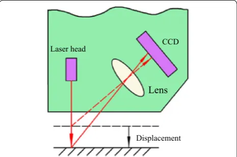
Additionally, the laser triangulation displacement sen-sor can be divided into four categories: specular reflec-tion type, diffuse reflecreflec-tion type, spectral interference type and confocal reflection type. Ref. [11] gives detail experimental comparison and analysis of the four types. The specular reflection type requires very high measured surface quality. The spectral interference type and con-focal reflection type have high measuring precision, but the measuring range is limited. Finally, the micro-epsilon ILD 2220 diffuse reflection type with measuring range of 50 ± 10  mm, resolution of 0.3  μm and measuring rates of 10  kHz is selected for the spline shaft measurement system. Note that the resolution of the laser displace-ment sensor is 0.3 μm, divided by the dimensional change about 20 μm, thus, the measuring error is estimated 1.5%, which meets the usage requirements. The measurement principle of the diffuse reflection type sensor is shown in Figure 3.

4 Data Acquisition and Processing

4.1 Acquisition of the Data

Before measuring, calibration of the distance from laser displacement sensor to the workpiece axis is needed. The calibration process is as follows: first, the standard cylindrical test bar is clamped on the spindle. Second, the laser displacement is adjusted to locate in an appropriate distance to the test bar and within the measuring range. It is important to make sure the workpiece axis and the laser line at the same height. Third, by measuring the test bar, the distance Lm from laser displacement sensor to

the cylindrical surface of the workpiece is obtained. Then, the distance from laser displacement sensor to the work-piece axis can be calculated by:

Angle Worktable

Spline shaft Spindle

Laser beam

Rotary encoder

LDS DAQ card

Computer Displacement

Figure 2 Schematic diagram of the measurement system

Laser head

Displacement CCD

Lens

where R0 is the radius of the test bar.

During the measuring process, the spline shaft rotates at a constant speed. At the same time, the laser displace-ment sensor transmits pulses by 10000/s. In each pulse, the distance Lt from laser displacement sensor to the surface of the workpiece is measured and a certain rota-tion angle θt is recorded by rotary encoder simultane-ously. The data of rotation angle θt and the distance Lt are stored to the computer as a vector (θt, Lt). Then, the cal-culation software transfer (θt, Lt) to (θt, Rt) by equation:

where Rt is the distance from the surface of the workpiece to its axis, L0 is the distance from laser displacement sen-sor to the workpiece axis calibrated before.

In polar coordinate system, each vector (θt, Rt) repre-sents a point. Using tens of thousands of the points, the cross profile of the workpiece can be plotted precisely. When measuring the spline shaft, the cross profile is like a gear. Figure 4 shows the schematic and photograph of the experimental setup.

4.2 Recognition of the Tooth Roots

In the computer image processing, the feature points play a very important role in characteristic recognition. Feature points, such as angular point, tangency point and inflection point, are the basic units to characterize a specific shape. They can be applied to senior visual pro-cessing such as pattern recognition, shape matching and dimension measurement, etc. For the spline shaft measur-ing, the feature points are the tooth roots and tooth crests. At present, the commonly used feature point recog-nition algorithm includes: slope method, extremum method, chord to point distance accumulation method and curvature method [20]. However, they are too sen-sitive to the signal noise and have poor performance for an on machine measuring system, which has slight vibration during measurement (see Figure 5). Finally, a

(4)

L0 = R0 + Lm,

(5) Rt = L0 − Lt,

multipoint curvature method with robust recognition performance is developed.

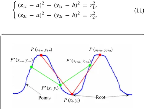
Curvature is the rate of change (at a point) of the angle between a curve and a tangent to the curve. The greater the curvature, the sharper the line bend. Based on the phenomenon that curvature on feature point changes dramatically, the feature point can be recog-nized when given a threshold. In the curvature method, continuous three points and their coordinate values are used to calculate the curvature of each point on a line. But, its curvature calculation range is too nar-row to avoid the effect of vibration. This problem can be handled by the multipoint curvature method, which expands its curvature calculation range thus showing robust recognition performance. In fact, the value cal-culated by multipoint curvature method is not the true curvature of a point, but an approximate value.

The curvature equation can be given as follows:

For discrete data sets: P =

Pi(xi,yi)|0 ≤ i ≤ n

, the difference calculation is used as a substitute for the differential calculation. Let the curvature calculation range be 2n+ 1, then

where

where (xi, yi) is the coordinate value of a point, (xi–n, yi–n)

is n points before it, (xi+n, yi+n) is n points after it. Then, (6)

Ki = y′′_i

(1 + y′_i2)3/2.

(7) 

  

  

y′_i = yi+n − yi−n xi+n − xi−n ,

y′′_i = y

′

i+n − y

′

i−n

xi+n − xi−n ,

(8)

y′_i+n =

yi+n − yi

xi+n − xi

, y′_i−n =

yi − yi−n

xi − xi−n ,

Spline shaft Laser beam

LDS ILD 2000

Lt

Rt

L0 ¹

Pillar

LDS Spline shaft

Rolling device

Figure 4 Schematics and photograph of the experimental setup

0 1 2 3 4 5 6

22.5 23.0 23.5 24.0 24.5 25.0 25.5

Radiu

s

R

/m

m

Measured profile Real profile

Angleθ /rad

the calculation equation by using multipoint curvature method would be:

The n value has great influence on the curvature Ki. A certain n value should be given to obtain the maximum curvature when calculating. In fact, it can be determined by equation:

where j is the number of all points, i is the number of the root of a spline shaft. In this case, when the point P

is located in the bottom of tooth root, its curvature Ki

reaches the maximum value, i.e., it is bigger than any other adjacent point such as the green point P’ shown in Figure 6.

4.3 Calculation of the Dimensional Change

In rolling, the dimensional change is determined by the rolling pressure rather than the cutting depth as in turn-ing or millturn-ing. So, it is hard to know the actual dimen-sional change ΔR (within 20 μm) of each tooth root. To solve this problem, a joint least square fitting method of the tooth root circle and tooth crest circle is used, which is upgraded from normally used least squares method. It is essential to fit the tooth root circle and the tooth crest circle jointly to enhance the fitting precision, otherwise, the center points of them would not be the same. Before fitting, the polar coordinate vector (θt, Rt) is converted to the rectangular coordinate vector (xi, yi) firstly. Then, the equations of tooth root circle and tooth crest circle can be presented as:

(9) Ki =

(yi+n−yi)(xi−xi−n)−(yi−yi−n)(xi+n−xi) (xx+n−xi)(xi−xi−n)(xi+n−xi−n)

1 +

yi+n−yi−n

xi+n−xi−n 23/2

.

(10) n = [j/2i].

(11)

(x1i − a)2 + (y1i − b)2 = r12,

(x2i − a)2 + (y2i − b)2 = r22,

where (x1i, y1i) are the points of tooth crest in

rectangu-lar coordinate system, (x2i, y2i) are the points of tooth

root in rectangular coordinate system, parameter (a, b) is the center point of them, parameter r1 is the radius of tooth crest circle, parameter r2 is the radius of tooth root circle.

According to the joint least square fit method, the residual sum of squares would be:

Let:

Then, the parameters can be calculated by:

(12)

J(a,b,r1,r2) =

n

i=1

[(x1i −a)2 +(y1i −b)2 −r12]2

+

n

i=1

[(x2i −a)2+(y2i −b)2 −r22]2.

(13)                                                                                   

p=n1 n

�

i=1

x_1i2 −

� _n

�

i=1

x1i

�2 +n2

n

�

i=1

x_2i2 −

� _n � i=1 x2i �2 ,

q =n1 n

�

i=1

y2_1i−

� _n

�

i=1

y1i

�2 +n2

n

�

i=1

y2_2i−

� _n � i=1 y2i �2 ,

s=n1 n

�

i=1

x_1i3 +n1 n

�

i=1

x1iy21i − n

�

i=1 (x21i+y

2 1i)

n

�

i=1

x1i

+n2 n

�

i=1

x3_2i+n2 n

�

i=1

x2iy22i− n

�

i=1

(x2_2i +y2_2i) n

�

i=1

x2i,

t =n1 n

�

i=1

y3_1i+n1 n

�

i=1

x21iy1i− n

�

i=1 (x21i +y

2 1i)

n

�

i=1

y1i

+n2 n

�

i=1

y3_2i +n2 n

�

i=1

x_2i2y2i − n

�

i=1

(x2_2i+y2_2i) n

�

i=1

y2i,

u =n1 n

�

i=1

x1iy1i − n � i=1 x1i n � i=1

y1i +n2 n

�

i=1

x2iy2i

− n

�

i=1

x2i n

�

i=1

y2i,

(14)                             

a = sq − tu

2(pq − u2₎,

b = tp− su

2(pq − u2₎,

r1 = 1 n1 n � i=1 �

(x1i − a)2+(y1i − b)2,

r2 = 1 n2

n �

i=1

�

(x2i − a)2+(y2i − b)2,

P(xi-n, yi-n) P(xi+n, yi+n)

P(xi, yi)

P'(xi-n, yi-n) P'(xi+n, yi+n)

P'(xi, yi)

Points Root

where n1 is the number of points of tooth crest circle, n2 is the number of points of tooth root circle. According to the fitted parameters before and after processing, the dimensional change ΔR can be calculated by:

where r’2 is the radius of tooth root circle after rolling process.

5 Experimental Results and Discussions

By using the measurement prototype established, a spline shaft with 48 teeth is scanned. The radius of tooth root circle and tooth crest circle are 23.09 mm and 24.87 mm, respectively. The system sampling frequency is 10  kHz. After the workpiece rotated 360°, a total of 14880 data points were collected, which took 1.5 s. To reduce the influence of rotation positioning error, the data were meas-ured when the shaft rotating reaches a constant speed and then one cycle of the data were recorded. Figure 7 shows the fitting figure and photograph of the spline shaft.

5.1 Calculation Result

Figure 8 shows the calculation result using the measuring data presented above. The first curve is the partial profile of the section contour. The other three curves below are the curvatures calculated with different n values (n= 21,

(15) R = r2′ − r2,

121, 221, respectively). The curvature of the curve bend-ing along anti-clockwise direction is positive (the case of tooth root), while along clockwise direction is negative (the case of tooth crest). It can be seen from the figure that as the n value increases, the sensibility of the mul-tipoint curvature method to the noise decreases, which means the recognition performance is better. But when the n value is too large, e.g., n= 221, some feature points may be judged as noise and failed to be recognized. So, it is important to determine the n value. Actually, it is influ-enced by the number of data points and the number of the root of a spline shaft.

In this measuring test, j= 14880, i= 48, so

n= [j/2i] = 155. Figure 9 shows the calculation result with

n= 155. It can be seen from the figure that the feature points separated significantly. All the tooth root points are above the line of Ki= 0, and all the tooth crest points are under the line of Ki= 0. With this result, it is easy to get all the angles of tooth root and tooth crest (take an average of the angle values for the points with curvature values greater than 400). From Figure 9, it can be seen that the multipoint curvature method is robust and sig-nificant in tooth feature recognition. Figure 10 shows the influence of n on radius fitting result. It also can be seen that the fitting result becomes inaccurate when n is too small (less than 60) or too large (more than 210), while

n= 155 locates in a suitable position.

The angle values of tooth roots calculated by program are shown in Table 1. In the table, i is the index number,

a Fitting figure bSection photograph

90 ₆₀

30

0

330

300 270 240 210 180

150 120

5 15

25

Figure 7 Fitting figure and photograph of the section

3.5 4 4.5 5

23 24 25

Radius R/m

m

3.5 4 4.5 5

Ѹ5000 500

3.5 4 4.5 5

Ѹ5000 500

3.5 4 4.5 5

Ѹ5000 500

Angleθ /rad

n=121

n=221

n=21

Curvature

K

i

Figure 8 Influence of n on curvature value K

0 1 2 3 4 5 6

−800 −600 −400 −2000 200 400 600 800

Curvatur

e

Ki

Angleθ /rad

Figure 9 Curvature value of each point when n= 155

0 100 200 300 24.87

24.88 24.89

n 0 100 200 300

23.07 23.08 23.09 23.10

n

Fitting result of

r1tonvalue

n=155 n=155

Crest circle radius

r1

/m

m Fitting result of

r2tonvalue

Root

circle radius

r2

/mm

θi is the angle values of the ith tooth root, Δθi=θi+1 −θi,

the average value is: Δθ= 2π/48 = 0.131  rad. It can be seen that the angle spacing values between two adjacent roots are evenly distributed. The angle spacing accuracy is 0.131 ± 0.001  rad for this measurement test result (including the manufacturing error of workpiece and the error of measurement instrument).

5.2 Results of Joint Least Squares Fitting

Figure 11 shows the fitting results of the tooth root cir-cle and the tooth crest circir-cle, which are showed with red dashed lines. The feature points are shown with red dots. Here, r1 is the radius of the tooth crest circle and r2 is the radius of the tooth root circle, (a, b) is the center point of the spline shaft.

To assess the measuring precision, four sections of the spline shaft were measured and each section was meas-ured 6 times. The results are shown in Table 2. It shows

that the repositioning accuracy (less than 0.6 μm) is good enough to measure the dimensional change. It’s worth noting that the value of r1 increases linearly and the value of r2 decreases linearly as the offset value c increases, which can be seen in Figure 12. The formulas were obtained by the linear least squares fitting of the experi-ment data. According to the formulas, when the offset value c= 0, the true value is obtained: r1= 24.872  mm and r2= 23.088 mm, respectively.

Table 1 Angles of the tooth roots

Note: θi is the angle value of the ith tooth root, Δθi=θi+1 − θi

i θi (rad) Δθi (rad) i θi (rad) Δθi (rad) i θi (rad) Δθi (rad)

1 0.075 0.131 17 2.174 0.131 33 4.262 0.130 2 0.206 0.131 18 2.305 0.130 34 4.392 0.131 3 0.337 0.132 19 2.435 0.130 35 4.523 0.131 4 0.469 0.131 20 2.565 0.130 36 4.654 0.131 5 0.601 0.131 21 2.695 0.131 37 4.785 0.132 6 0.732 0.131 22 2.827 0.131 38 4.916 0.132 7 0.863 0.131 23 2.958 0.131 39 5.048 0.131 8 0.993 0.131 24 3.089 0.131 40 5.179 0.131 9 1.124 0.131 25 3.220 0.130 41 5.309 0.131 10 1.255 0.132 26 3.349 0.130 42 5.441 0.132 11 1.387 0.132 27 3.480 0.130 43 5.573 0.132 12 1.519 0.131 28 3.610 0.130 44 5.705 0.132 13 1.651 0.130 29 3.740 0.130 45 5.836 0.131 14 1.781 0.131 30 3.870 0.131 46 5.967 0.131 15 1.911 0.131 31 4.001 0.131 47 6.098 0.130 16 2.043 0.131 32 4.132 0.130 48 6.228 0.130

5 15

25

30

210

60

240 90

270 120

300 150

330

180 0

r1

r2

O (a,b)

Figure 11 Fitting results of the tooth root and tooth crest circle

Table 2 Parameters fitting results for each section

Note: c= (a2_+b2₎1/2

Section Offset Crest circle radius Root circle radius

c (mm) r1 (mm) r2 (mm)

1 0.0127 ± 0.0005 24.8831 ± 0.0006 23.0695 ± 0.0003 2 0.0156 ± 0.0003 24.8867 ± 0.0006 23.0657 ± 0.0005 3 0.0183 ± 0.0013 24.8905 ± 0.0005 23.0602 ± 0.0006 4 0.0257 ± 0.0007 24.8958 ± 0.0009 23.0509 ± 0.0005

0.01 0.02 0.03 24.882

24.886 24.890 24.894 24.898

Offsetc/ mm

r1= 0.961c+24.872

0.01 0.02 0.03 23.050

23.054 23.058 23.062 23.066 23.070

Offsetc/ mm

r2=Ѹ1.443c+23.088

Fitting data Fitting line Fitting data

Fitting line

Crest circle radius

r1

/m

m

Root

circle radius

r2

/m

m

The dimensional change of the tooth roots can be achieved by calculating the radius of tooth root circle before and after rolling. The relationship between the dimensional change and the residual stress should be established by rolling experiments in the future. Accord-ingly, the spline shaft rolling performance can be rapidly evaluated using the dimensional change as an alterna-tive evaluation parameter. It is also worth noting that a hydraulic servo system should be used to generate accu-rate pressures in the future experiments and the residual stress will be measured using the X-ray diffraction (XRD).

6 Conclusions

(1) An on-machine non-contact measurement method for spline shaft rolling performance evaluation is proposed. To verify the validity of this method, a measurement prototype mainly consisted of a laser displacement sensor and rotary encoder was built on a rolling machine. Using the prototype estab-lished, a spline shaft is scanned and its section fig-ure is obtained.

(2) Through multipoint curvature method (MCM) and joint least square fitting method, the roots of the spline shaft were recognized automatically. The dimensional change can be calculated by fitting the radius of the tooth root circle before and after rolling. The offset error was also analyzed and cali-brated in data processing.

(3) Measurement test results show that the proposed method is feasible with high measurement preci-sion (radius measuring error less than 0.6 μm), high measurement efficiency (measuring time less than 2 s) and automatic control ability (auto evaluation of rolling performance). Moreover, the method can cover the measurement needs of different spline shafts and has potential to analyze various gears machining process.

Authors’ Contributions

Z‑QL and X‑BW were in charge of the whole trial; H‑WL and J‑JP wrote the manuscript; LJ and L‑JX assisted with sampling and laboratory analyses. All authors read and approved the final manuscript.

Author details

1 _{Key Laboratory of Fundamental Science for Advanced Machining, Beijing} Institute of Technology, Beijing 100081, China. 2 _{Beijing North Vehicle Group} Corporation, Beijing 100072, China.

Authors’ Information

Hong‑Wei Li, born in 1974, is currently a PhD candidate at Key Laboratory of Fundamental Science for Advanced Machining, Beijing Institute of Technology, China. He also is currently a researcher at Beijing North Vehicle Group Corpora-tion, China. His research interests include advanced machining technology, and rolling and measurement. E‑mail: [email protected].

Zhi‑Qiang Liang, born in 1984, is currently an associate professor at Key Laboratory of Fundamental Science for Advanced Machining, Beijing Institute of Technology, China. He received his PhD degree on mechanical engineer‑ ing from Beijing Institute of Technology, China, in 2011. His research interests

include advanced machining technology, cutting and grinding technique. Tel: +86‑10‑68911214; E‑mail: [email protected].

Jia‑Jie Pei, born in 1987, is currently a PhD candidate at Key Laboratory of Fundamental Science for advanced Machining, Beijing Institute of Technology, China. His research interests include advanced machining technology. E‑mail: [email protected].

Li Jiao, born in 1975, is currently an associate professor at Key Laboratory of Fundamental Science for Advanced Machining, Beijing Institute of Technology, China. She received his PhD degree on mechanical engineering from Beijing Institute of Technology, China, in 2002. His main research interests include high efficiency machining technology, digital process planning, rapid production preparation and group technology. E‑mail: [email protected].

Li‑Jing Xie, born in 1971, is currently an associate professor at Key Laboratory of Fundamental Science for Advanced Machining, Beijing Institute of Technology, China. She received his PhD degree on mechanical engineering from Karlsruhe Institute of Technology, Germany, in 2004. His main research interests include cutting and grinding of difficult‑to‑cut materials, ultra‑high speed cutting, database of high efficiency processing technology. E‑mail: [email protected].

Xi‑Bin Wang, born in 1958, is currently a professor and a PhD candidate supervisor at Key Laboratory of Fundamental Science for Advanced Machining, Beijing Institute of Technology, China. He received his PhD degree on mechani‑ cal engineering from Xi’an Jiaotong University, China, in 1994. His main research interests include advanced machining technology, grinding, cutting and green manufacturing. E‑mail: [email protected].

Competing Interests

The authors declare that they have no competing interests.

Funding

Supported by Industrial Technology Development Program of China (Grant Nos. JCKY2017208C005, A0920132008), and National Natural Science Founda‑ tion of China (Grant No. 51575049).

Publisher’s Note

Springer Nature remains neutral with regard to jurisdictional claims in pub‑ lished maps and institutional affiliations.

Received: 30 August 2016 Accepted: 6 August 2018

References

[1] A V Guimaraesa, P C Brasileirob, G C Giovanni, et al. Failure analysis of a half‑shaft of a formula SAE racing car. Case Studies in Engineering Failure Analysis, 2016, 7: 17–23.

[2] I Barsoum, F Khan, Z Barsoum. Analysis of the torsional strength of hard‑ ened splined shafts. Materials and Design, 2014, 54: 130–136.

[3] L J Shen, A Lohrengel, G Schäfer. Plain–fretting fatigue competition and prediction in spline shaft‑hub connection. International Journal of Fatigue, 2013, 52: 68–81.

[4] Y J Li, W F Zhang, C H Tao. Fracture analysis of a castellated shaft. Engi-neering Failure Analysis, 2007, 14: 573–578.

[5] N S Rossini, M Dassisti, K Y Benyounis, et al. Methods of measuring residual stresses in components. Materials and Design, 2012, 35: 572–588. [6] K Guptaa, R F Laubschera, P J Davimb, et al. Recent developments in sus‑ tainable manufacturing of gears: a review. Journal of Cleaner Production, 2016, 112(4): 3320–3330.

[7] Y C Zhang, J X Han, X B Fu, et al. Measurement and control technology of the size for large hot forgings. Measurement, 2014, 49: 52–59.

[8] J Rejc, U Cinkelj, M Munih. Dimensional measurements of a gray‑iron object using a robot and a laser displacement sensor. Robotics and Computer-Integrated Manufacturing, 2009, 25: 155–167.

[10] J H Sun, J Zhang, Z Liu. A vision measurement model of laser displace‑ ment sensor and its calibration method. Optics and Lasers in Engineering, 2013, 51: 1344–1352.

[11] C Hong, S Ibarkai. Non‑contact R‑test with laser displacement sensors for error calibration of five‑axis machine tools. Precision Engineering, 2013, 37: 159–171.

[12] Y Kondo, K Hasegawa, H Kawamata, et al. On‑machine non‑contact dimension‑measurement system with laser displacement sensor for vane‑tip machining of RFQs. Nuclear Instruments and Methods in Physics Research A, 2012, 667: 5–10.

[13] F M Zhang, X H Qu, J F Ouyang. An automated inner dimensional meas‑ urement system based on a laser displacement sensor for long‑stepped pipes. Sensors, 2012, 12: 5824–5834.

[14] Y C Tan, Z M Ripin. Technique of measuring piston secondary motion using laser displacement sensors. Experimental Mechanics, 2012, 52: 1447–1459.

[15] E S Gadelmawla. Computer vision algorithms for measurement and inspection of spur gears. Measurement, 2011, 44: 1669–1678.

[16] M A Younes, A M Khalil, M N Damir. Automatic measurement of spur‑gear dimensions using laser light. Part 1: measurement of tooth thickness and pitch. Optical Engineering, 2005, 44: 1–13.

[17] P F Su, L J Wang, M Komori. Design of laser interferometric system for measurement of gear tooth flank. Optic, 2011, 122: 1301–1304. [18] W Gao, M Furukawa, S Kiyono. Cutting error measurement of flexspline

gears of harmonic speed reducers using laser probes. Precision Engineer-ing, 2004, 28: 358–363.

[19] E J Hearn. Mechanics of materials volume 1: an introduction to the mechanics of elastic and plastic deformation of solids and structural materials. 3rd ed. Musselburgh: Butterworth‑Heinemann; 1997. [20] J H Han, T Poston. Chord‑to‑point distance accumulation and planar cur‑