ISSN: 2146-4138 www.econjournals.com
122
Determination of Sovereign Rating: Factor Based Ordered
Probit Models for Panel Data Analysis Modelling Framework
Dilek Teker (corresponding author)
Faculty of Economics and Administrative Sciences, Okan University, Turkey. Email: [email protected]
Aynur Pala
Research Analyst, Research Centre for Financial Risks, Okan University, Turkey. Email: [email protected]
Oya Kent
Research Assistant, Research Centre for Financial Risks, Okan University, Turkey. Email: [email protected]
ABSTRACT: The aim of this research is to compose a new rating methodology and provide credit notches to 23 countries which of 13 are developed and 10 are emerging. There are various literature that explains the determinants of credit ratings. Following the literature, we select 11 variables for our model which of 5 are eliminated by the factor analysis. We use specific dummies to investigate the structural breaks in time and cross section such as pre crises, post crises, BRIC membership, EU membership, OPEC membership, shipbuilder country and platinum reserved country. Then we run an ordered probit model and give credit notches to the countries. We use FITCH ratings as benchmark. Thus, at the end we compare the notches of FITCH with the ones we derive out of our estimated model.
Keywords: Credit notches; factor analysis; ordered probit model JEL Classifications: G01; G23
1. Introduction
123 2. Literature Review
The rating agencies evaluate many factors ranging from solvency factors affecting the ability to repay the debt to socio-political factors that might influence the willingness to pay off the borrower. Cantor and Packer (1996) may be regarded as an earlier study in this area, analyzing the determinants and impact of sovereign credit ratings using a cross-section of 49 countries by applying OLS methodology. In their analysis, six factors appear to play an important role in determining a country’s rating: per capita income, GDP growth, inflation, external debt, level of economic development, and default history. Their findings do not support a statistically significant relationship between ratings and either fiscal or current account deficits. In fact, the empirical literature on sovereign ratings only extends in a few strands. The preliminary work in this field generally employs linear regression methods in examining the determinants of country risks. These studies include Afonso (2003), Alexe et al. (2003), and Butler and Fauver (2006). The study of Afonso (2003) examines possible determinants of sovereign credit ratings assigned by Moody’s and the S&P for a sample of 81 countries consisting of 29 developed and 52 developing countries for the year 2001 by using the OLS method. Rating scales are transformed by using linear, logistic and exponential transformations. The variables that have statistically significant explanatory power for the rating levels are GDP per capita, external debt as a percentage of exports, the level of economic development, default history, real growth rate, and the inflation rate. The results of the logistic transformation estimations appear to be better for the overall samples, especially for the countries located at the top end of the rating scale. Alexe et al. (2003) intends to develop a transparent, consistent, self-contained, and stable system which will closely approximate the major existing country risk rating systems. They selected the Standard & Poor country risk rating system as a benchmark for the desired system. The variables concerned are nine economic variables (GDP per capita, inflation rate, trade balance, international reserves, fiscal balance, export growth rate, debt to GDP, financial depth and efficiency, and exchange rate) and three political variables (political stability, government effectiveness and corruption levels). The data covers 69 countries (24 industrialized countries, 11 Eastern European countries, 8 Asian countries, 10 Middle Eastern countries, 15 Latin American countries and South Africa) for the year 1998. A non-recursive, multiple regression model is applied as an estimation method to the data by its non-reliance on any information derived from the lagged ratings. Their results show that there is a high level of correlation between predicted and actual ratings. Butler and Fauver (2006) examine the cross-sectional determinants of sovereign credit ratings by using a sample of 86 countries as of March 2004. The main findings of the study display that the quality of a country’s legal and political institutions, which are measured by its rule of law, political stability, voice of the people, corruption control, government effectiveness, or regulatory quality, has a vital role in determining these ratings. Strikingly, credit ratings are found to be over three times as sensitive to a change in the legal environment composite as they are to GDP per capita, inflation, foreign debt per GDP, and overall economic development. Linear panel models generalizing a cross section specification to panel data are also used by Monfort and Mulder (2000), Eliasson (2002), and Canuto et al. (2012).
However, since ratings are discrete and ordinal in nature, traditional estimation techniques on a linear representation of the ratings are not appropriate. One problem that arises by using OLS is that it implicitly assumes that the difference between any two adjacent categories is always equal. Besides, even if this is true, in the presence of elements in the top and bottom category, the coefficient estimates are still biased, even in large samples (Afonso et al., 2011) To overcome this critique, another strand of the literature estimates the determinants of sovereign debt ratings under a limited dependent variable framework, for instance Hu et al. (2002), Bissoondoyal-Bheenick (2005) and Afonso et al. (2007, 2009, 2011).
124 foreign reserves, and net exports/GDP. In addition to these economic variables, the sample of the 25 highest rated countries includes the unemployment rates as well as unit labour costs. For the 70 lowest rated countries, in addition to the economic variables used for the full sample of countries, current account balance/GDP and foreign debt/GDP are included instead of net export/GDP since these two additional variables reflect the level of debt of these for countries in this category. The most striking discovery of the study is that the relevance of specific economic variables and financial variables can vary according to the level of development in any country. The results of the three samples of countries indicate that the economic variables do not play an important role for the higher rated sample of countries, while on the other hand for the lower rated countries in addition to GNP per capita and inflation, the current account balance and the level of foreign reserves do play an important role in determining sovereign ratings.
Afonso et al., (2007) employ panel estimations and random effects ordered probit approaches to assess the explanatory power of several macroeconomic and public governance variables in determining sovereign debt credit ratings for the period of 1995-2005 for 78 countries. Findings from the panel’s random effects framework displayed a set of core variables that are relevant for the determination of the ratings per capita GDP, GDP real growth rate, government debt, government effectiveness, external debt and external reserves, and sovereign default indicators. The ordered probit analysis confirmed the overall estimation results from the linear panel regressions. Another relevant outcome of the study shows that low rating levels are more affected by external debt and external reserves while inflation plays a bigger role for high rating levels. In another study of Afonso et al. (2009), researching the determinants of sovereign debt ratings for 66 countries for the period of 1996-2005, they employed ordered logit and probit plus random effects ordered probit approaches. Random effects ordered probit estimation is more efficient than the other two methods, since a considerable number of variables show up as significant that are not picked up using the other two methods. A very recent study conducted by the same authors (Afonso et al., 2011) tries to distinguish between short-run and long-run determinants of a country’s rating using linear and ordered response models. Results show that changes in GDP per capita, GDP growth, government debt, and government balance have a short-run impact on a country’s credit rating, while government effectiveness, external debt, foreign reserves, and default history are important long-run determinants. There is also an extending branch of work using alternative statistical methods to traditional ones, such as artificial neural networks, self organizing maps, hierarchical cluster analysis, etc.
Yim and Mitchell (2005) investigate the ability of new statistical techniques in predicting country risk ratings. Hybrid artificial neural network analysis is applied to a sample of 20 high risk and 32 low risk countries for the year 2002 and compared with the traditional models such as discriminant analysis, logit, probit models and ordinary neural network models. To analyze the country’s risks with visual effects, hierarchical cluster analysis and self-organizing maps are investigated as well. The results obtained show that hybrid neural networks out-perform all other models applied in the study.
Bennell et al. (2006) also compare the performance of ordered probit models and artificial neural networks (ANN) in predicting sovereign ratings using a dataset of 11 rating agencies and 70 countries over the period of 1989–1999. The paper demonstrates that ANN represents a superior technology for calibrating and predicting sovereign ratings relative to ordered probit modelling.
Another study by Bissoondoyal-Bheenick et al., (2006) focuses on the use of a different approach called case-based reasoning (CBR) in modeling sovereign ratings. The CBR system, broadly defined, is the process of solving new problems based on the solutions of similar past problems. The paper compares ordered probit models, CBR and results obtained to indicate that they are similar in terms of the significance of variables and forecast accuracy. In addition to this, the study includes a proxy for technological development, particularly mobile phone use; both models show that it is of great importance.
125 3. Data and Methodology
The aim of this research is to compose a new rating methodology and give credit notches to 23 countries which are members of G-20 and the countries named as PIGS countries1. Some econometric techniques are implemented to provide notches and at the end we compare the estimated results with FITCH ratings. Based on the evidence in existing literature, a set of variables that may determine sovereign ratings are specified as: Real GDP growth (G), GDP per capita (GPC), inflation (CPI), public debt/GDP (PD), budget balance/GDP (BD), foreign reserves/GDP (RES), foreign direct investment/GDP (FDI), portfolio investment/GDP (PORTF), current account balance/GDP (CA), Economic Freedom Index (EFI) and Corruption Perception Index (COR). In this study, we conduct an ordered probit model in which the dependent variable is a sovereign rating for a panel of selected countries. As a novelty, we specify the explanatory variables by using a factor analysis technique. Therefore, the initial step is the implementation of this factor analysis. Factor analysis seeks to discover if the observed variables can be explained largely or entirely in terms of a much smaller number of variables which are called factors. Factor analysis provides us an empirical basis in creating fewer but independent variables out of many highly correlated variables. Another virtue of using this technique lies behind the fact that it relieves us of the problem of multicollinearity among the explanatory variables as the factors are not correlated while variables included in these factors are. The results of the factor analysis provided us with six homogenous factor groups reduced from 11 variables2. Once the factors are determined, an ordered probit approach in which the cut-off points divide each category is estimated by the model. Probit is the probability unit which is then transformed into its cumulative probability value from a normal distribution. An ordered probit model is:
y∗=xi'tβ + γZ + ε
where y∗ is an unobservable latent variable that measures the creditworthiness of a countryi in period t. xit is a vector of time varying explanatory variables and is a vector of unknown parameters. Zit contains time invariant regressors that are generally dummy variables and is a random disturbance term. If the distribution of is chosen to be normal, then ultimately this produces an ordered probit model. As usual, yit* is unobserved. What we assume here is that yi* is related to the observed variable yi, which is the Fitch rating in this case, in the following way:
= 0 ∗< τ 1 < ∗< τ 2 < ∗< τ 3 < ∗< τ 4 < ∗< τ 5 < ∗< τ
.. ..
23 < ∗< 0
where the τ (τ < τ < τ < ⋯ < τ ) are known threshold parameters to be estimated.
The following model may be named as factor ordered probit model, wherey∗ is an unobservable latent variable that measures the credit-worthiness of a country i in period t. Fit is a vector of factors derived from factor analysis and is a vector of unknown parameters. Zit contains time invariant regressors that are generally dummy variables and is a random disturbance term.
y∗=Fit'β + γZ + δ(F ∗ Z) + ε
Regarding a rating schedule, estimation results will be expressed in a 1-24point scale, and then we perform a linear transformation to the letter grades assigned by FITCH. The ratings by FITCH are replaced by a numerical equivalent grade, on a scale from 1 to 24, as shown in Appendix 1.
1
G-20: Argentina, Australia, Brazil, Canada, China, France, Germany, India, Indonesia, Italy, Japan, Mexico, Russia, Saudi Arabia, South Africa, South Korea, Turkey, UK, USA.
PIGS: Portugal, Greece, Ireland, Spain
2
126 4. Empirical Results
4.1. Factor ordered probit model results
By using a panel data set of 23 countries for 13 years (1998-2010), an ordered probit model is estimated where a dependent variable is the transformed rating categories on a scale of 1-24 and independent variables are shown. Following this, explanatory variables are reduced by exploring factor analysis which is used as new independent variables in ordered probit regressions. Factor ordered probit regressions are then estimated. The possibility of structural breaks in time and cross-section dimensions is examined through the incorporation of appropriate dummy information into the factor ordered probit regression.
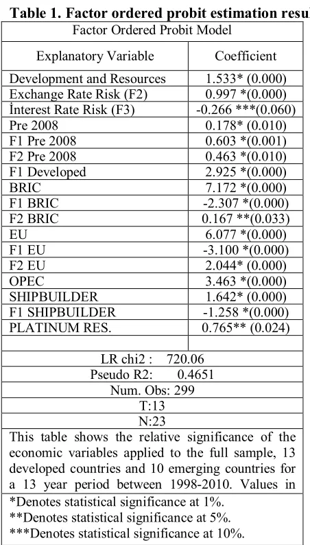
In order to investigate the structural breaks in time and cross-section dimension, we define additional dummies in the model. For structural breaks in time dimension, we include a dummy for the European debt crisis in the year 2008 (pre-crisis=1 post-crisis=0), while in the cross-section dimension, we define dummies according to their outstanding profile of the country such as being a BRIC country, an EU country, an OPEC country, a shipbuilder country and a platinum reserved country. Both breaks in intercept and trend are examined throughout the analysis. Interaction terms are also included in the estimation. Table 1 shows the relative significance of the economic variables and across the rating categories applied to the full sample; it shows 13 developed countries (8 EU) and 10 emerging countries (4 BRIC) for a period of 13 years from 1998-2010.
Ordered probit estimation results show GPC, CPI, PD, EFI, CORR and PORTF variables are statistically significant at a 95% confidence level. But this result is basically due to the multicollineratiy problem among the regressors which tend to produce a lower standard errors and hence higher t-statistics. In order to cope with this problem, we invoke statistical factor analysis techniques to get more homogenous explanatory variables reduced in fewer factor groups. Data set covering a 13 year period of 11 explanatory variables is subjected to factor analysis. In this framework, the Kaiser-Meyer-Olkin (KMO) test is explored to examine the sampling adequacy which should be greater than 0.5 for a satisfactory factor analysis to proceed, which was determined to be 0.678 and concluded that the sampling is adequate.
Our factor analysis provided us with six homogenous factor groups reduced from eleven variables. Taking into account the factor loadings taken on by variables, we observe that GPC, CORR, EFI and RES variables have factor loadings exceeding 0.5 and are loaded in factor F1. Notice that the first factor accounts for 59% of the total variance. We may call this factor the F1 “level of development and resources”. The BD variable is loaded in factor F2 alone and accounts for 29% of the total variance. This factor may be called an “exchange rate risk”. Public Deficit/GDP is included in factor F3, accounting for 17% of the total variance and may be called as “interest rate risk”. Other variables are not loaded in any factor with factor ladings less than 0.5.
In determining the number of factors to be used in the study, we employed the criteria of eigenvalue which has to be greater than 1. The eigenvalues of the factors F1, F2 and F3 are 3.14; 1.52 and 0.69 respectively. These selected factors account for 100% of the total variance. Although factor F3 has an eigenvalue lower than 1, it is included in the model since it increases the significance and predictive power of the model. As a last step, these factors are transformed into indexes and are then used as explanatory variables in the model. Ordered probit embodied in factor model form is estimated through maximum likelihood estimation (MLE).
Y∗=F1it' +F2it' β +F3it'β + P2008 γ + F1P2008 γ + F2P2008 γ +
δ + 1 δ + 2 δ +
+ 1 + 2 + 3
+ 1 + 2 + 3 +
+ 1 + 2 + 3 +
+ 1 + 2 + 3 +
127 Table 1. Factor ordered probit estimation results
Factor Ordered Probit Model
Explanatory Variable Coefficient
Development and Resources 1.533* (0.000)
Exchange Rate Risk (F2) 0.997 *(0.000)
İnterest Rate Risk (F3) -0.266 ***(0.060)
Pre 2008 0.178* (0.010)
F1 Pre 2008 0.603 *(0.001)
F2 Pre 2008 0.463 *(0.010)
F1 Developed 2.925 *(0.000)
BRIC 7.172 *(0.000)
F1 BRIC -2.307 *(0.000)
F2 BRIC 0.167 **(0.033)
EU 6.077 *(0.000)
F1 EU -3.100 *(0.000)
F2 EU 2.044* (0.000)
OPEC 3.463 *(0.000)
SHIPBUILDER 1.642* (0.000)
F1 SHIPBUILDER -1.258 *(0.000)
PLATINUM RES. 0.765** (0.024)
LR chi2 : 720.06 Pseudo R2: 0.4651
Num. Obs: 299 T:13 N:23
This table shows the relative significance of the economic variables applied to the full sample, 13 developed countries and 10 emerging countries for a 13 year period between 1998-2010. Values in parenthesisare p-values.
*Denotes statistical significance at 1%. **Denotes statistical significance at 5%. ***Denotes statistical significance at 10%.
In the model, factors F1, F2 and F3 are positive and statistically level at the conventional confidence levels. The pre-crisis dummy (P2008) has a negative sign and was found to be statistically significant which reveals that the global financial crisis lead to a change/break (shift in level) in the mean value of the sovereign credit ratings. In other words, the crisis has brought about a permanent change in the levels of the credit ratings. When we examine the effect of the 2008 crisis on the slope of coefficients, we observe a structural break in F1 and F2 factors for all countries while there is no structural change in F3. In other words, the effect of F1 and F2 on sovereign ratings differ significantly in pre and post crisis periods in terms of both content and load, while F3 has a stable effect over time.3 There is no significant difference between the developed and developing countries’ ratings in terms of mean values. But we observe a differentiation in slope of the F1 countries which can be seen in the interaction term (F1*Developed). What this finding tells us is that whether a country is developed or not does not create a differentiation in the mean value of ratings, while for developed countries, the F1 factor provides a differentiation in the positive direction with a coefficient of 2.92. It also shows us that this differentiation is not permanent due to the break in the slope. This asserts that the changes in developing countries’ economies may cause this advantage to vanish. The effects of F2 and F3 do not differ across developed and developing countries. The differentiation in these factors may be expected to rise much more in sub-groups. Hence, the dummy for BRIC countries, which takes place among the developing countries, is positively signed and statistically significant in explaining rating grades. The mean value of rating grades of BRIC countries significantly differs in levels from others, which signifies a permanent advantage to them. In BRIC countries, F1 has a negative
3
128 significant effect on ratings while F2 has a positive significant effect. Thus, rating grades of BRIC countries differ both in levels and in the slopes of F1 and F2 relative to other countries. Results indicate that being an EU country also calls forth a significant difference in average rating grades in the positive direction. EU membership provides a permanent and appreciable advantage to countries in respect to rating grades. In EU countries, F1 has a negative significant effect on ratings while F2 effects are significantly positive.
In EU countries, the effects of F1 and F2 on sovereign ratings differ significantly relative to other countries in terms of both content and load; however the effect of F3 resembles other countries. Underground resource abundance measured by things such as OPEC membership and Platinum reserves are also observed to be influential variables in determining credit ratings. On the other hand, maritime transportation is the most important means of transport in the global trade of mine and petroleum. In this regard, Korea, China and Japan as leaders in world shipbuilding, have a rating grade advantage over other countries. In shipbuilding countries, the effect of F1 on ratings is negative and statistically significant. In these countries, the F1 factor differs in terms of content and effect relative to other countries. Finally South Africa, having 90% of the world platinum reserves, particularly has a permanent advantage in average ratings over other countries due to the fact that platinum is the most valuable substance mined following gold. In other words, there has been a shift in average value4.
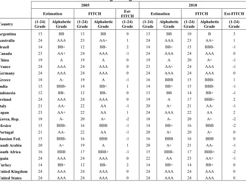
4.2. Estimation of sovereign rating notches
With the help of the above model, we have estimated sovereign ratings for the years of 2005 and 2010. Rating estimates are given in Table 2 in a 2-scale basis (1-24 scale and letter grade) compared with the FITCH ratings. Table 2 indicates that FITCH ratings differ in terms of criteria and weight, as well as in respect to some countries, between these two years. Germany, Australia, France, Canada, Brazil, China and India are among the countries that FITCH overrated. According to our findings, Korea, Ireland, Greece, Italy, Turkey, Russia, South Africa, Saudi Arabia, and Argentina are underrated by FITCH. Rating margins between the estimated and the actual FITCH rating and between 2005 and 2010 that are within the 0-1 range include countries such as the United States, Portugal, Japan, the United Kingdom, Mexico, Spain and Indonesia.
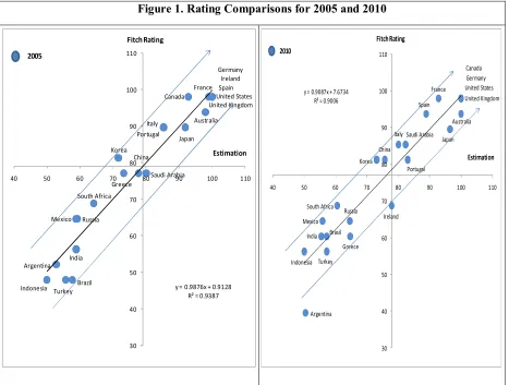
Figure 1 compares the estimated and actual values for 2005 in a scatter plot. The explanatory power of the estimated and the actual value is 94%, which is quite high. According to the scatter plot, 11 of the 23 countries are rated above the average while 10 of them are rated below average. This situation indicates a transition period for these countries in question and a new process of classification among countries. Hence, this transition will be observed in analysis related to 2010. In 2005, Greece was the sole country that was rated below the A notch among the G20 and PIGS countries. When we analyse the rating scatter plot which has undergone a reshaping in the aftermath of the 2008 crisis, the differentiation caused by the financial crisis in the EU area draws attention. Expansionary monetary policies implemented as a crisis recovery strategy in developed countries have paved the way for the 2010 EU debt crisis for those whose budget balances have been depreciated by these policies. Countries which did not have substantial reserves such as Greece, Ireland, Portugal and Spain, had a rating score advantage by virtue of being EU members. This might be seen as the main reason for the failing economics following the 2008 debt crisis. Structural change triggered by the crisis is seen more clearly with the differentiation of PIGS countries in the rating scores scatter graph. In the end, this perceptibly demonstrated that there were deficiencies in determining accession criteria and in the process of establishing the union. Thus, a legal control process has been initiated and has cleared the way for ruling out the countries of the union which do not meet the criteria. This is a more reliable step for the sake of perpetuity of the union. Developing countries, as distinct from developed ones, have implemented fiscal tightening precautions besides expansionary policies. This provided them with a well-functioning growth, as well as budget and debt balances and hence an improvement in their status as seen in Figure 1. The positions of developing countries have ameliorated relative to their scatter graph in 2005.
4
129 Table 2. Sovereign rating estimates
2005 2010
Estimation FITCH
Est-FITCH Estimation FITCH Est-FITCH
Country Grade (1-24) Alphabetic Grade Grade (1-24) Alphabetic Grade Grade (1-24) Grade (1-24) Alphabetic Grade Grade (1-24) Alphabetic Grade Grade (1-24)
Argentina 13 BB 13 BB 0 13 BB 10 B 3
Australia 24 AAA 23 AA+ 1 24 AAA 23 AA+ 1
Brazil 14 BB+ 12 BB- 2 14 BB+ 15 BBB- -1
Canada 23 AA+ 24 AAA -1 24 AAA 24 AAA 0
China 19 A 19 A 0 19 A 20 A+ -1
France 24 AAA 24 AAA 0 23 AA+ 24 AAA -1
Germany 24 AAA 24 AAA 0 24 AAA 24 AAA 0
Greece 18 A- 19 A -1 16 BBB 15 BBB- 1
India 15 BBB- 14 BB+ 1 14 BB+ 15 BBB- -1
Indonesia 12 BB- 12 BB- 0 13 BB 14 BB+ -1
Ireland 24 AAA 24 AAA 0 19 A 17 BBB+ 2
Italy 21 AA- 22 AA -1 20 A+ 21 AA- -1
Japan 23 AA+ 22 AA 1 24 AAA 22 AA 2
Korea, Rep. 18 A- 20 A+ -2 18 A- 20 A+ -2
Mexico 15 BBB- 16 BBB -1 14 BB+ 16 BBB -2
Portugal 21 AA- 22 AA -1 20 A+ 20 A+ 0
Russian Fed. 15 BBB- 16 BBB -1 16 BBB 16 BBB 0
Saudi Arabia 20 A+ 19 A 1 20 A+ 21 AA- -1
South Africa 16 BBB 17 BBB+ -1 15 BBB- 17 BBB+ -2
Spain 24 AAA 24 AAA 0 22 AA 23 AA+ -1
Turkey 14 BB+ 12 BB- 2 14 BB+ 14 BB+ 0
United Kingdom 24 AAA 24 AAA 0 24 AAA 24 AAA 0
United States 24 AAA 24 AAA 0 24 AAA 24 AAA 0
5. Conclusion
In the aftermath of the global financial crisis faced in 2008, developed and developing countries have implemented diverse monetary and fiscal policies to recover, which has led to a differentiation in economic indicators across country groups. This differentiation required rating agencies to modify criteria and weights used in their risk evaluation and it implies to define a new structure. It is a well known fact that BRIC countries exhibit a more diverse structure among the developing economies. “C of BRIC” – China, is gradually getting more differentiated with its significant amount of export and foreign currency reserves among the other BRIC countries and therefore, recent country classification issues are going to be debated.
130 Argentina Australia Brazil Canada China France United Kingdom Korea Indonesia India Germany Ireland Italy Japan Greece Mexico Portugal Russia Saudi Arabia South Africa Turkey United States Spain
y = 0.9876x + 0.9128 R² = 0.9387
30 40 50 60 70 80 90 100 110
40 50 60 70 80 90 100 110
Estimation Fitch Rating 2005 Argentina Australia Brasil United States China France United Kingdom Greece India Indonesia Ireland Portugal Japan Korea Mexico Saudi Arabia Russia Italy South Africa Spain Turkey Germany Canada
y = 0.9087x + 7.6734 R² = 0.9006
30 40 50 60 70 80 90 100 110
40 50 60 70 80 90 100 110
Estimation Fitch Rating
2010
Figure 1. Rating Comparisons for 2005 and 2010
References
Afonso, A. (2003), Understanding the determinants of sovereign debt ratings: Evidence for the two leading agencies. Journal of Economics and Finance, 27(1), 56–74.
Afonso, A., Gomes, P.M., Rother, P. (2007), What hides behind sovereign debt ratings. ECB Working Paper No. 711
Afonso, A., Gomes, P.M., Rother, P. (2009), Ordered response models for sovereign debt ratings. Applied Economics Letters, 16(8), 769–773.
Afonso, A., Gomes, P.M., Rother, P. (2011), Short and long-run determinants of sovereign debt credit ratings. International Journal of Finance & Economics, 16(1), 1–15.
Alexe, S., Hammer, P.L., Kogan, A., Lejeune, M.A. (2003), A non-recursive regression model for country risk rating. RUTCOR-Rutgers University Research Report RRR, 9, 1–40.
Bennell, J.A., Crabbe, D., Thomas, S., Gwilym, O. (2006), Modelling sovereign credit ratings: Neural Networks versus ordered probit. Expert Systems with Applications, 30(3), 415–425.
Bissoondoyal-Bheenick, E. (2005), An analysis of the determinants of sovereign ratings. Global Finance Journal, 15(3), 251-280.
Bissoondoyal-Bheenick, E., Brooks, R., Yip, A.Y.N. (2006), Determinants of sovereign ratings: A comparison of case-based reasoning and ordered probit approaches. Global Finance Journal, 17(1), 136–154.
Butler, A.W., Fauver, L. (2006), Institutional environment and sovereign credit ratings. Financial Management, 35(3), 53–79.
Cantor, R., Packer, F. (1996), Determinants and impact of sovereign credit ratings. Economic Policy Review, 2(2), 37-54.
131 Eliasson, A.C. (2002), Sovereign credit ratings. Deutche Bank Research, Research notes in economics
& statistics No. 02-1, http://hdl.handle.net/10419/40267
Ferri, G., Liu, L.G., Majnoni, G. (2001), The role of rating agency assessments in less developed countries: Impact of the proposed Basel guidelines. Journal of Banking & Finance, 25(1), 115– 148.
Hammer, P.L., Kogan, A., Lejeune, M.A. (2006), Modelling country risk ratings using partial orders. European Journal of Operational Research, 175(2), 836–859.
Hu, Y.T., Kiesel, R., Perraudin, W. (2002), The estimation of transition matrices for sovereign credit ratings. Journal of Banking & Finance, 26(7), 1383–1406.
Monfort, B., Mulder, C.B. (2000), Using Credit Ratings for Capital Requirements on Lending to Emerging Market Economies: Possible Impact of a New Basel Accord. IMF Working Paper No.00/69.
Yim, J., Mitchell, H. (2005), Comparison of country risk models: Hybrid neural networks, logit models, discriminant analysis and cluster techniques. Expert Systems with Applications, 28(1), 137–148.
Appendix 1. Linear transformation of ratings
Appendix 2- Factor Analysis
Factor Analysis is used mostly for data reduction purposes, for instance to get a small set of variables from a large set of variables and to create indexes with variables that measure similar things. Factor analysis assumes that all the rating data on different attributes can be reduced down to a few important dimensions. The statistical algorithm deconstructs the rating (raw score) into its various components, and reconstructs the partial scores into underlying factor scores. The degree of correlation between the initial raw score and the final factor score is called a factor loading.
Suppose for some unknown constants and unobserved random variables , where ∈ 1, … , and ∈ 1, … , ,
where < , we have;
− = + … + +
for the full sample where;
is the ith country’s score for the kth subject
the mean of the country’s scores for the kth subject (assumed to be zero)
is the ith country’s "development indicator",
is the ith country’s "currency risk indicator”,
is the ith country’s “interest rate risk indicator”
FITCH Rating Rating Grade (1-24)
AAA 24
AA+ 23
AA 22
AA- 21
A+ 20
A 19
A- 18
BBB+ 17
BBB 16
BBB- 15
BB+ 14
BB 13
BB- 12
B+ 11
B 10
B- 9
CCC+ 8
CCC 7
CCC- 6
CC 5
C 4
DDD 3
DD 2
132 l are the factor loadings for the kth subject, for = 1, ...,p
ε is the difference between the ith country's score in the kth subject and the averages core in the kth subject of all country whose levels of development and currency risk are the same as those of the ith country,
Factor analysis mainly requires four stages. At the first stage, variables are selected and an inter correlation matrix is generated for all of the variables included. Kaiser–Meyer–Olkin (KMO) test is applied to the variables in question in order to validate if the variables are factorable. The KMO value should be greater than 0.5 for a satisfactory factor analysis. At the second stage, an appropriate number of components are extracted from the correlation matrix based on the initial solution. In the initial solution, each variable is standardised to have a mean of 0.0 and a standard deviation of 1.0. Thus, the eigenvalue of the factor should be greater than or equal to 1.0, if it is to be extracted. In this study we will extract the factors that are greater than 1, but at some circumstances, such as the existence of factors that have significant effect on ratings but have eigenvalue less than 1, this limit may be brought down. If the interpretation of the factors is ambiguous, that is if one or more variables load about the same on more than one factor, then factors are rotated in order to clarify the relationship between the variables and the factors. Various methods can be used for factor rotation, the Varimax method is the most commonly used one. As a last stage results are then derived by analysing the factor load of each variable. Factor load is selected based on the criteria that it should be greater than 0.5and maximum among the factors greater then 0.5. Then, appropriate names are given to each factor by considering the factor loads.
A2. Table 1. Results of Factor Analysis
Full Sample (FS)- Principle Factor Analysis
Explanatory Variables
Factor Loading
KMO Test
Unrotated Factors
Eigen
Value Proportion Cum.
GPC 0.850** 0.671
F1** 3.147 0.591 0.591
EFİ 0.801** 0.723
CORR 0.845** 0.785
RES -0.538** 0.774
BD 0.671** 0.634 F2** 1.525 0.287 0.878
PD 0.525** 0.636 F3 0.694 0.130 1.008
CPI -0.317 0.471
FDI 0.341 0.771
PORTF 0.368 0.503
G 0.271 0.560
CA -0.485 0.654