Mean Field Variational Approximation for Continuous-Time Bayesian Networks

Mean Field Variational Approximation

for Continuous-Time Bayesian Networks

∗

Ido Cohn† IDO [email protected]

Tal El-Hay† _{TALE@CS.HUJI.AC.IL}

Nir Friedman [email protected]

School of Computer Science and Engineering The Hebrew University

Jerusalem 91904, Israel

Raz Kupferman [email protected]

Institute of Mathematics The Hebrew University Jerusalem 91904, Israel

Editor: Manfred Opper

Abstract

Continuous-time Bayesian networks is a natural structured representation language for

multi-component stochastic processes that evolve continuously over time. Despite the compact represen-tation provided by this language, inference in such models is intractable even in relatively simple structured networks. We introduce a mean field variational approximation in which we use a prod-uct of inhomogeneous Markov processes to approximate a joint distribution over trajectories. This variational approach leads to a globally consistent distribution, which can be efficiently queried. Additionally, it provides a lower bound on the probability of observations, thus making it attractive for learning tasks. Here we describe the theoretical foundations for the approximation, an efficient implementation that exploits the wide range of highly optimized ordinary differential equations (ODE) solvers, experimentally explore characterizations of processes for which this approximation is suitable, and show applications to a large-scale real-world inference problem.

Keywords: continuous time Markov processes, continuous time Bayesian networks, variational

approximations, mean field approximation

1. Introduction

Many real-life processes can be naturally thought of as evolving continuously in time. Examples cover a diverse range, starting with classical and modern physics, but also including robotics (Ng et al., 2005), computer networks (Simma et al., 2008), social networks (Fan and Shelton, 2009), gene expression (Lipshtat et al., 2005), biological evolution (El-Hay et al., 2006), and ecological systems (Opper and Sanguinetti, 2007). A joint characteristic of all above examples is that they are complex systems composed of multiple components (e.g., many servers in a server farm and multiple residues in a protein sequence). To realistically model such processes and use them in

∗. A preliminary version of this paper appeared in the Proceedings of the Twenty Fifth Conference on Uncertainty in Artificial Intelligence, 2009 (UAI 09).

making sensible predictions we need to learn how to reason about systems that are composed of multiple components and evolve continuously in time.

Generally, when an evolving system is modeled with sufficient detail, its evolution in time is Markovian; meaning that its future state it determined by its present state—whether in a deter-ministic or random sense—independently of its past states. A traditional approach to modeling a multi-component Markovian process is to discretize the entire time interval into regular time slices of fixed length and represent its evolution using a Dynamic Bayesian network, which compactly represents probabilistic transitions between consecutive time slices (Dean and Kanazawa, 1989; Murphy, 2002; Koller and Friedman, 2009). However, as thoroughly explained in Nodelman et al. (2003), discretization of a time interval often leads either to modeling inaccuracies or to an unnec-essary computational overhead. Therefore, in recent years there is a growing interest in modeling and reasoning about multi-component stochastic processes in continuous time (Nodelman et al., 2002; Ng et al., 2005; Rajaram et al., 2005; Gopalratnam et al., 2005; Opper and Sanguinetti, 2007; Archambeau et al., 2007; Simma et al., 2008).

In this paper we focus on continuous-time Markov processes having a discrete product state

space S=S1×S2× · · · ×SD, where D is the number of components and the size of each Si is

finite. The dynamics of such processes that are also time-homogeneous can be determined by a single rate matrix whose entries encode transition rates among states. However, as the size of the state space is exponential in the number of components so does the size of the transition matrix. Continuous-time Bayesian networks (CTBNs) provide an elegant and compact representation lan-guage for multi-component processes that have a sparse pattern of interactions (Nodelman et al., 2002). Such patterns are encoded in CTBNs using a directed graph whose nodes represent com-ponents and edges represent direct influences among them. The instantaneous dynamics of each component depends only on the state of its parents in the graph, allowing a representation whose size scales linearly with the number of components and exponentially only with the indegree of the nodes of the graph.

Inference in multi-component temporal models is a notoriously hard problem (Koller and Fried-man, 2009). Similar to the situation in discrete time processes, inference in CTBNs is exponential in the number of components, even with sparse interactions (Nodelman et al., 2002). Thus, we have to resort to approximate inference methods. The recent literature has adapted several strategies from discrete graphical models to CTBNs in a manner that attempts to exploit the continuous-time representation, thereby avoiding the drawbacks of discretizing the model.

One class of approximations includes sampling-based approaches, where Fan and Shelton (2008) introduce a likelihood-weighted sampling scheme, and more recently El-Hay et al. (2008) introduce a Gibbs-sampling procedure. The complexity of the Gibbs sampling procedure has been shown to naturally adapt to the rate of each individual component. Additionally it yields more accurate answers with the investment of additional computation. However, it is hard to bound the required time in advance, tune the stopping criteria, or estimate the error of the approximation.

neces-sarily form a globally consistent distribution. Third, it is restricted to approximations in the form of piecewise-homogeneous messages on each interval. Thus, the refinement of the number of in-tervals depends on the fit of such homogeneous approximations to the target process. Finally, the approximation of Nodelman et al does not provide a provable approximation on the likelihood of the observation—a crucial component in learning procedures.

Here, we develop an alternative variational approximation, which provides a different trade-off. We use the strategy of structured variational approximations in graphical models (Jordan et al., 1999), and specifically the variational approach of Opper and Sanguinetti (2007) for approximate inference in latent Markov Jump Processes, a related class of models (see below for more elaborate comparison). The resulting procedure approximates the posterior distribution of the CTBN as a product of independent components, each of which is an inhomogeneous continuous-time Markov process. We introduce a novel representation that is both natural and allows numerically stable com-putations. By using this representation, we derive an iterative variational procedure that employs passing information between neighboring components as well as solving a small set of differential equations (ODEs) in each iteration. The latter allows us to employ highly optimized standard ODE solvers in the implementation. Such solvers use an adaptive step size, which as we show is more efficient than any fixed time interval approximation.

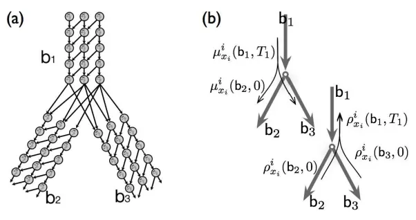
We finally describe how to extend the proposed procedure to branching processes and particu-larly to models of molecular evolution, which describe historical dynamics of biological sequences that employ many interacting components. Our experiments on this domain demonstrate that our procedure provides a good approximation both for the likelihood of the evidence and for the ex-pected sufficient statistics. In particular, the approximation provides a lower-bound on the likeli-hood, and thus is attractive for use in learning.

The paper is organized as follows: In Section 2 we review continuous-time models and inference problems in such models. Section 3 introduces a general variational principle for inference using a novel parameterization. In Section 4 we apply this principle to a family of factored representations and show how to find an optimal approximation within this family. Section 5 discusses related work. Section 6 gives an initial evaluation. Section 7 presents branching process and further experiments, and Section 8 discusses our results.

2. Foundations

CTBNs are based on the framework of continuous-time Markov processes (CTMPs). In this section we begin by briefly describing CTMPs. See, for example, Gardiner (2004) and Chung (1960) for a thorough introduction. Next we review the semantics of CTBNs. We then discuss inference problems in CTBNs and the challenges they pose.

2.1 Continuous Time Markov Processes

A continuous-time stochastic process with state space S is an uncountable collection of S-valued random variables{X(t)_{: t≥0}where X}(t)_{describes the state of the system at time t. Systems with}

multiple components are described by state spaces that are Cartesian products of spaces, Si, each

A continuous-time Markov process is a continuous-time stochastic process in which the joint distribution of every finite subset of random variables X(t0)_,X(t1)_{, . . . ,X}(tK)_{, where t0<t1<· · ·<t}

K, satisfies the conditional independence property, also known as the Markov property:

Pr(X(tK)=xK|X(tK−1)=xK−1, . . . ,X(t0)=x0) =Pr(X(tK)=xK|X(tK−1)=xK−1).

In simple terms, the knowledge of the state of the system at a certain time make its states at later times independent of its states at former times. In that case the distribution of the process is fully determined by the conditional probabilities of random variable pairs Pr(X(t+s)=y|X(s)_{=x), namely,}

by the probability that the process is in state y at time t+s given that is was in state x at time s, for all 0≤s<t and x,y∈S. A CTMP is called time homogeneous if these conditional probabilities do not depend on s but only on the length of the time interval t, thus, the distribution of the process is determined by the Markov transition functions,

px,y(t)≡Pr(X(t+s)=y|X(s)=x), for all x,y∈S and t≥0,

which for every fixed t can be viewed as the entries of a stochastic matrix indexed by states x and y. Under mild assumptions on the Markov transition functions px,y(t), these functions are differ-entiable. Their derivatives at t=0,

qx,y= lim t→0+

px,y(t)−11x=y

t ,

are the entries of the rate matrixQ, where11 is the indicator function. This rate matrix describes the infinitesimal transition probabilities,

px,y(h) =11x=y+qx,yh+o(h), (1)

where o(·)means decay to zero faster than its argument, that is limh↓0o(_hh) =0. Note that the

off-diagonal entries ofQare non-negative, whereas each of its rows sums up to zero, namely,

qx,x=−

∑

y6=x

qx,y.

The derivative of the Markov transition function for t other than 0 satisfies the so-called forward, or master equation,

d

dtpx,y(t) =

∑

_z qz,ypx,z(t). (2)

A similar characterization for the time-dependent probability distribution, p(t), whose entries are defined by

px(t) =Pr(X(t)=x), x∈S,

is obtained by multiplying the Markov transition function by entries of the initial distribution p(0)

and marginalizing, resulting in

d

dtp=pQ. (3)

The solution of this ODE is

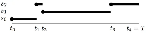
Figure 1: An example of a CTMP trajectory: The process starts at state x1 =s0, transitions to x2=s2at t1, to x3=s1at t2, and finally to x4=s2at t3.

where exp(tQ)is a matrix exponential, defined for any square matrixAby the Taylor series,

exp(A) =I+

∞

∑

k=1 Ak

k! .

Applying this solution to the initial condition px′(0) =11_x=x′, we can express the Markov transition

function px,y(t)using the rate matrixQas

px,y(t) = [exp(tQ)]_x,y. (4)

Although a CTMP is an uncountable collection of random variables (the state of the system at every time t), a trajectoryσof{X(t)_}

t≥0over a time interval[0,T]can be characterized by a finite number of transitions K, a sequence of states (x0,x1, . . . ,xK) and a sequence of transition times

(t0=0,t1, . . . ,tK,tK+1=T). We denote byσ(t)the state at time t, that is,σ(t) =xkfor tk≤t<tk+1. Figure 1 illustrates such a trajectory.

2.2 Multi-component Representation - Continuous-Time Bayesian Networks

Equation (4) indicates that the distribution of a homogeneous Markov process is fully determined

by an initial distribution and a single rate matrix Q. However, since the number of states in a

D-component Markov Process is exponential in D, an explicit representation of this transition matrix is often infeasible. Continuous-time Bayesian networks are a compact representation of Markov processes that satisfy two assumptions. First it is assumed that only one component can change at a time, thus transition rates involving simultaneous changes of two or more components are zero. Sec-ond, the transition rate of each component i depends only on the state of some subset of components denoted Pai⊆ {1, . . . ,D} \ {i}and on its own state. This dependency is represented using a directed graph, where the nodes are indexed by{1, . . . ,D}and the parent nodes of i are Pai(Nodelman et al., 2002). With each component i we then associate a conditional rate matrixQi|Pai

·|ui for each state uiof

Pai. The off-diagonal entries qi_xi|Pa_,yii_|ui represent the rate at which Xi transitions from state xi to state

yi given that its parents are in state ui. The diagonal entries are q i|Pai

xi,xi|ui =−∑yi6=xiq i|Pai

xi,yi|ui,ensuring that each row in each conditional rate matrix sums up to zero. The dynamics of X(t)are defined by a rate matrixQwith entries qx,y, which combines the conditional rate matrices as follows:

qx,y=



 

 

qi|Pai

xi,yi|ui δ(x,y) ={i} ∑iqi|Pai

xi,xi|ui x=y

0 otherwise,

whereδ(x,y) ={j|xj6=yj}denotes the set of components in which x differs from y.

To have another perspective on CTBN’s, we may consider a discrete-time approximation of

the process. Let h be a sampling interval. The subset of random variables{Xtk : k≥0}, where

tk =k h, is a discrete-time Markov process over a D-dimensional state-space. Dynamic Bayesian networks (DBNs) provide a compact modeling language for such processes, namely the conditional distribution of a DBN Ph(X(tk+1)|X(tk))is factorized into a product of conditional distributions of X(tk+1)

i given the state of a subset of X(tk)∪X(tk+1). When h is sufficiently small, the CTBN can be

approximated by a DBN whose parameters depend on the rate matrixQof the CTBN ,

Ph(X(tk+1)=y|X(tk)=x) = D

∏

i=1 Ph(X(

tk+1)

i =yi|X( tk)

i =xi,U(tk)=ui), (6)

where

Ph(X( tk+1)

i =yi|X( tk)

i =xi,U(tk)=ui) =11xi=yi+q i|Pai

xi,yi|uih. (7)

Each such term is the local conditional probability that X(tk+1)

i =yi given the state of Xi and Ui at time tk. These are valid conditional distributions, because they are non-negative and are normalized, that is

∑

yi∈Si

11xi=yi+qi_xi|Pa_,yii_|uih

=1

for every xi and ui. Note that in this discretized process, transition probabilities involving changes

in more than one component are o(h), as in the CTBN. Moreover, using Equations (1) and (5) we

observe that

Pr(X(tk+1)=y|X(tk)=x) =Ph(X(tk+1)=y|X(tk)=x) +o(h).

(See Appendix A for detailed derivations). Therefore, the CTBN and the approximating DBN are

asymptotically equivalent as h→0.

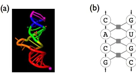
Example 1 An example of a multi-component process is the dynamic Ising model, which

corre-sponds to a CTBN in which every component can be in one of two states, −1 or+1, and each

component prefers to be in the same state as its neighbor. These models are governed by two

parameters: a coupling parameterβ(it is the inverse temperature in physical models, which

deter-mines the strength of the coupling between two neighboring components), and a rate parameterτ,

which determines the propensity of each component to change its state. Low values ofβcorrespond

to weak coupling (high temperature). More formally, we define the conditional rate matrices as

qi|Pai xi,yi|ui =τ

1+e−2yiβ∑j∈Paixj−1

where xj∈ {−1,1}. This model is derived by plugging the Ising grid to Continuous-Time Markov

Networks, which are the undirected counterparts of CTBNs (El-Hay et al., 2006).

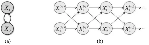
Consider a two component Ising model whose structure and corresponding DBN are shown in Figure 2. This system is symmetric, that is, the conditional rate matrices are identical for i∈ {1,2}.

As an example, for a specific choice ofβandτwe have:

Qi|Pai

·|−1 =

- +

- −1 1

+ 10 −10

Qi|Pai

·|+1 =

- +

- −10 10

(a) (b)

Figure 2: Two representations of a two binary component dynamic process. (a) The associated CTBN. (b) The DBN corresponding to the CTBN in (a). The models are equivalent when h→0.

The local conditional distributions of the DBN can be directly inferred from Equation (7). For example

Ph(X( tk+1)

1 =1|X

(tk)

1 =−1,X

(tk)

2 =1) =10h.

Here, in both components the conditional rates are higher for transitions into states that are identical to the state of their parent. Therefore, the two components have a disposition of being in the same state. To support this intuition, we examine the amalgamated rate matrix:

Q =

- - - + + - + +

- - −2 1 1 0

- + 10 −20 0 10

+ - 10 0 −20 10

+ + 0 1 1 −2.

Clearly, transition rates into states in which both components have the same value is higher. Higher transitions rate imply higher transition probabilities, for example:

p-+,--(h) = 10 h+o(h),

p--,-+(h) = h+o(h).

Thus the probability of transitions into a coherent state is much higher than into an incoherent state.

2.3 Inference in Continuous-time Markov Processes

Our setting is as follows: we receive evidence of the states of several or all components within a time interval[0,T]. The two possible types of evidence that may be given are continuous evidence, where we know the state of a subset U⊆X continuously over some sub-interval[t1,t2]⊆[0,T], and point evidence of the state of U at some point t∈[0,T]. For convenience we restrict our treatment to a time interval[0,T]with full end-point evidence X(0)=e0and X(T)=eT. We shall discuss the more general case in Section 5.

conditional expectations of statistics that involve entire trajectories of the process. Two important examples for queries are the sufficient statistics required for learning. These statistics are the amount of time in which Xi is in state xi and Pai are in state ui, and the number of transitions that Xi un-derwent from xi to yi while its parents were in state ui (Nodelman et al., 2003). We denote these statistics by T_xii_|ui and Mi_xi,yi|ui respectively. For example, in the trajectory of the univariate process in Figure 1, we have Ts2 =t2−t1+t4−t3and Ms0,s2=1.

Exact calculation of these values is usually a computationally intractable task. For instance, calculation of marginals requires first calculating the pointwise distribution over X using a forward-backward like calculation:

Pr(X(t)=x|e0,eT) =

pe0,x(t)px,eT(T−t) pe0,eT(T)

, (8)

and then marginalizing

Pr(U(t)=u|e0,eT) =

∑

x\u

Pr(X(t)=x|e0,eT),

where px,y(t) = [exp(tQ)]x,y, and the size ofQis exponential in the number of components. More-over, calculating expected residence times and expected number of transitions involves integration over the time interval of these quantities (Nodelman et al., 2005a):

E[Tx] = 1 pe0,eT(T)

Z T

0

pe0,x(t)px,eT(T−t)dt,

E[Mx,y] = 1 pe0,eT(T)

Z T

0

pe0,x(t)qx,ypy,eT(T−t)dt .

These make this approach infeasible beyond a modest number of components, hence we have to resort to approximations.

3. Variational Principle for Continuous-Time Markov Processes

Variational approximations to structured models aim to approximate a complex distribution by a simpler one, which allows efficient inference. This problem can be viewed as an optimization problem: given a specific model and evidence, find the “best” approximation within a given class of simpler distributions. In this setting the inference is posed as a constrained optimization problem, where the constraints ensure that the parameters correspond to valid distributions consistent with the evidence. Specifically, the optimization problem is constructed by defining a lower bound to the log-likelihood of the evidence, where the gap between the bound and the true likelihood is the divergence of between the approximation and the true posterior. While the resulting problem is generally intractable, it enables us to derive approximate algorithms by approximating either the functional or the constrains that define the set of valid distributions. In this section we define the lower-bound functional in terms of a general continuous-time Markov process (that is, without assuming any network structure). Here we aim at defining a lower bound on ln PQ(eT|e0)as well as to approximating the posterior probability PQ(· |e0,eT), where PQis the distribution of the Markov

process whose instantaneous rate-matrix isQ. We start by examining the structure of the posterior

Recall that the distribution of a time-homogeneous Markov process is characterized by the con-ditional transition probabilities px,y(t), which in turn is fully redetermined by the constant rate matrixQ. It is not hard to see that whenever the prior distribution of a stochastic process is that of a homogeneous Markov process with rate matrixQ, then the posterior PQ(·|e0,eT)is also a Markov process, albeit generally not a homogeneous one. The distribution of a continuous-time Markov processes that is not homogeneous in time is determined by conditional transition probabilities, px,y(s,s+t), which depend explicitly on both initial and final times. These transition probabilities

can be expressed by means of a time-dependent matrix-valued function,R(t), which describes

in-stantaneous transition rates. The connection between the time-dependent rate matrixR(t) and the

transition probabilities, px,y(s,s+t)is established by the master equation,

d

dtpx,y(s,s+t) =

∑

_z rz,y(s+t)px,z(s,s+t),

where rz,y(t)are the entries ofR(t). This equation is a generalization of Equation (2) for inhomoge-neous processes. As in the homogeinhomoge-neous case, it leads to a master equation for the time-dependent probability distribution,

d

dtpx(t) =

∑

_y ry,x(t)py(t),

thereby generalizing Equation (3).

By the above discussion, it follows that the posterior process can be represented by a time-dependent rate matrixR(t). More precisely, writing the posterior transition probability using basic properties of conditional probabilities and the definition of the Markov transition function gives

PQ(X(t+h)=y|X(t)=x,X(T)=eT) =

px,y(h)py,eT(T−t+h) px,eT(T−t)

.

Taking the limit h→0 we obtain the instantaneous transition rate of the posterior process

rx,y(t) =lim h→0

PQ(X(t+h)=y|X(t)=x,X(T)=eT)

h =qx,y·

py,eT(T−t) px,eT(T−t)

. (9)

This representation, although natural, proves problematic in the framework of deterministic ev-idence because as t approaches T the transition rate into the observed state tends to infinity. In par-ticular, when x6=eT and y=eT, the posterior transition rate is qx,eT·

p_eT,_eT(T−t)

px,_eT(T−t). This term diverges

as t →T , because the numerator approaches 1 while the denominator approaches 0. We therefore consider an alternative parameterization for this inhomogeneous process that is more suitable for variational approximations.

3.1 Marginal Density Representation

Let Pr be the distribution of a Markov process, generally not time homogeneous. We define a family of functions:

µx(t) =Pr(X(t)=x),

γx,y(t) =lim h↓0

Pr(X(t)=x,X(t+h)=y)

h , x6=y.

The function µx(t)is the marginal probability that X(t)=x. The functionγx,y(t)is the probability density that X transitions from state x to y at time t. Note that this parameter is not a transition rate, but rather a product of a point-wise probability with the point-wise transition rate of the distribution, that is, the entries of the time-dependent rate matrix of an equivalent process can be defined by

rx,y(t) =

( _γ

x,y(t)

µx(t) µx(t)>0, 0 µx(t) =0.

(11)

Hence, unlike the (inhomogeneous) rate matrix at time t,γx,y(t)takes into account the probability of being in state x and not only the rate of transitions.

We aim to use the family of functions µ and γ as a representation of the posterior process.

To do so, we need to characterize the set of constraints that these functions satisfy. We begin by constraining the marginals µx(t) to be valid distributions that is, 0≤µx(t)≤1 and ∑xµx(t) =1. A similar constraint on the pairwise distributions implies thatγx,y(t)≥0 for x6=y. Next, we infer additional constraints from consistency properties between distributions over pairs of variables and their uni-variate marginals. Specifically, Equation (10) implies that for x6=y

Pr(X(t)=x,X(t+h)=y) =γx,y(t)h+o(h). (12)

Plugging this identity into the consistency constraint

µx(t) =Pr(X(t)=x) =

∑

y

Pr(X(t)=x,X(t+h)=y),

defining

γx,x(t) =−

∑

y6=x

γx,y(t)

and rearranging, we obtain

Pr(X(t)=x,X(t+h)=y) =11x=yµx(t) +γx,y(t)h+o(h), (13)

which unlike (12) is valid for all x,y. Marginalizing (13) with respect to the second variable,

Pr(X(t+h)=x) =

∑

y

Pr(X(t)=y,X(t+h)=x),

we obtain a forward update rule for the uni-variate marginals

µx(t+h) =µx(t) +h

∑

y

γy,x(t) +o(h).

Rearranging terms and taking the limit h→0 gives a differential equation for µx(t),

d

dtµx(t) =

∑

_y γy,x(t).

Definition 1 A familyη={µx(t),γx,y(t): 0≤t≤T}of functions is a Markov-consistent density set if the following constraints are fulfilled:

µx(t) ≥ 0,

∑

x

µx(0) =1,

γx,y(t) ≥ 0 ∀y6=x, γx,x(t) = −

∑

y6=x γx,y(t),

d

dtµx(t) =

∑

_y γy,x(t),

andγx,y(t) =0 whenever µx(t) =0. We denote by

M

the set of all Markov-consistent densities.

Using standard arguments we can show that there exists a correspondence between (generally

inhomogeneous) Markov processes and density setsη. Specifically, givenη, we construct a process

by defining an inhomogeneous rate matrix R(t) whose entries are defined in Equation (11) and

prove the following:

Lemma 2 Letη={µx(t),γx,y(t): 0≤t≤T}. Ifη∈

M

, then there exists a continuous-time Markov process Pr for which µxandγx,ysatisfy (10) for every t in the right-open interval [0,T).

Proof See appendix B

The converse is also true: for every integrable inhomogeneous rate matrixR(t) the corresponding

marginal density set is defined by _dtdµx(t) =∑yry,x(t)µy(t)andγx,y(t) =µx(t)rx,y(t). The processes we are interested in, however, have additional structure, as they correspond to the posterior distri-bution of a time-homogeneous process with end-point evidence. In that case, multiplying Equation (9) by µx(t)gives

γx,y(t) =µx(t)·qx,y·

py,eT(T−t) px,eT(T−t)

. (14)

Plugging in Equation (8) we obtain

γx,y(t) =

pe0,x(t)·qx,y·py,eT(T−t) p_e0,eT(T) ,

which is zero when y6=eT and t=T . This additional structure implies that we should only

con-sider a subset of

M

. Specifically the representationηcorresponding to the posterior distribution

PQ(·|e0,eT)satisfies µx(0) =11x=e0, µx(T) =11x=eT,γx,y(0) =0 for all x6=e0andγx,y(T) =0 for all

y6=eT. We denote by

M

e⊂

M

the subset that contains Markov-consistent density sets satisfying

these constraints. This analysis suggests that for every homogeneous rate matrix and point

evi-dence e there is a member in

M

_ethat corresponds to the posterior process. Thus, from now on we

restrict our attention to density sets from

M

_e.

3.2 Variational Principle

The marginal density representation allows us to state the variational principle for continuous pro-cesses, which closely tracks similar principles for discrete processes. Specifically, we define a

set is the log-likelihood of the evidence and is attained for a density set that represents the poste-rior distribution. This formulation will serve as a basis for the mean-field approximation, which is introduced in the next section.

Define a free energy functional,

F

(η;Q) =

E

(η;Q) +

H

(η),

which, as we will see, measures the quality ofηas an approximation of PQ(·|e). (For succinctness,

we will assume that the evidence e is clear from the context.) The two terms in the functional are the average energy,

E

(η;Q) =

Z T

0

∑

_x

"

µx(t)qx,x+

∑

y6=x

γx,y(t)ln qx,y

#

dt,

and the entropy,

H

(η) =

Z T

0

∑

_{x y}

∑

_6=xγx,y

(t)[1+ln µx(t)−lnγx,y(t)]dt.

The following theorem establishes the relation of this functional to the Kullback-Leibler (KL) divergence and the likelihood of the evidence, and thus allows us to cast the variational inference into an optimization problem.

Theorem 3 LetQbe a rate matrix, e= (e0,eT)be states of X , andη∈

M

e. Then

F

(η;Q) =ln PQ(eT|e0)−ID(Pη||PQ(·|e))

where Pη is the distribution corresponding toηandID(Pη||PQ(·|e))is the KL divergence between

the two processes.

We conclude from the non-negativity of the KL divergence that the energy functional

F

(η;Q)is

a lower bound of the log-likelihood of the evidence. The closer the approximation to the target posterior, the tighter the bound. Moreover, since the KL divergence is zero if and only if the two distributions are equal almost everywhere, finding the maximizer of this free energy is equivalent to finding the posterior distribution from which answers to different queries can be efficiently com-puted.

3.3 Proof of Theorem 3

We begin by examining properties of distributions of inhomogeneous Markov processes. Let X(t)be

an inhomogeneous Markov process with rate matrixR(t). As in the homogeneous case, a trajectory

σof{X(t)_}

t≥0over a time interval[0,T]can be characterized by a finite number of transitions K, a sequence of states(x0,x1, . . . ,xK) and a sequence of transition times (t0=0,t1, . . . ,tK,tK+1=T). We denote by Σ the set of all trajectories of X[0,T]. The distribution over Σ can be

character-ized by a collection of random variables that consists of the number of transitionsκ, a sequence

of states (χ0, . . . ,χκ) and transition times(τ1, . . . ,τκ). Note that the number of random variables

that characterize the trajectory is by itself a random variable. The density fR of a trajectory

σ={K,x0, . . . ,xK,t1, . . . ,tK} is the derivative of the joint distribution with respect to transition times, that is,

fR(σ) =

∂K ∂t1· · ·∂tK

which is given by

fR(σ) =px0(0)· K−1

∏

k=0

h

e

Rtk+1

tk rxk,_xk(t)dt_r

xk,xk+1(tk+1)

i

·eRtKtK+1rxK,xK(t)dt_.

For example, in caseR(t) =Qis a homogeneous rate matrix this equation reduces to

fQ(σ) =px0(0)· K−1

∏

k=0

h

eqxk,_xk(tk+1−tk)_q xk,xk+1

i

·eqxK,_xK(tK+1−tK)_.

The expectation of a random variableψ(σ)is an infinite sum (because one has to account for all

possible numbers of transitions) of finite dimensional integrals,

EfQ[ψ]≡

Z

ΣfR(σ)ψ(σ)dσ≡ ∞

∑

K=0

∑

x0 · · ·

∑

xK Z T

0 Z tK

0 · · ·

Z t2

0

fR(σ)ψ(σ)dt1· · ·dtK.

The KL-divergence between two densities that correspond to two inhomogeneous Markov pro-cesses with rate matricesR(t)andS(t)is

ID(fR||fS) =

Z

ΣfR(σ)ln

fR(σ)

fS(σ)

dσ . (15)

We will use the convention 0 ln 0=0 and assume the support of fSis contained in the support of fR.

That is fR(σ) =0 whenever fS(σ) =0. The KL-divergence satisfiesID(fR||fS)≥0 and is exactly

zero if and only if fR= fSalmost everywhere (Kullback and Leibler, 1951).

Let η∈

M

_e be a marginal density set consistent with e. As we have seen, this density set

corresponds to a Markov process with rate matrixR(t)whose entries are defined by Equation (11), hence we identify f_η≡ fR.

Given evidence e on some event we denote fQ(σ,e)≡ fQ(σ)·11σ|=e, and note that

PQ(e) =

Z

{σ:σ|=e}fQ(σ)dσ=

Z

ΣfQ(σ,e)dσ ,

whereσ|=e is a predicate which is true ifσis consistent with the evidence. The density function of the posterior distribution PQ(·|e)satisfies fS(σ) = fQ_PQ(σ_(e,e₎) whereS(t)is the time-dependent rate

matrix that corresponds to the posterior process. Manipulating (15), we get

ID(f_η||fS) =

Z

Σ fη(σ)ln fη(σ)dσ−

Z

Σfη(σ)ln fS(σ)dσ≡Efη[ln fη(σ)]−Efη[ln fS(σ)].

Replacing ln fS(σ)by ln fQ(σ,e)−ln PQ(e)and applying simple arithmetic operations gives

ln PQ(e) =Efη[ln fQ(σ,e)]−Efη[ln fη(σ)] +ID(fη||fS).

The crux of the proof is in showing that the expectations in the right-hand side satisfy

and

−Efη[ln fη(σ)] =

H

(η),

implying that

F

(η;Q)is a lower bound on the log-probability of evidence with equality if and only if f_η= fQalmost everywhere.

To prove these identities for the energy and entropy, we treat trajectories as functionsσ:

R

→

R

where

R

is the set of real numbers by denotingσ(t)≡X(t)(σ)—the state of the system at time t. Using this notation we introduce two lemmas that allow us to replace integration over a set of trajectories by a one dimensional integral, which is defined over a time variable. The first result handles expectations of functions that depend on specific states:

Lemma 4 Letψ: S×

R

→

R

be a function, then

Efη Z _T

0

ψ(σ(t),t)dt

=

Z T

0

∑

_x

µx(t)ψ(x,t)dt.

Proof See Appendix C.1

As an example, by settingψ(x′,t) =11x′_=x we obtain that the expected residence time in state x is

Efη[Tx] =R0Tµx(t)dt. The second result handles expectations of functions that depend on transitions between states:

Lemma 5 Letψ(x,y,t)be a function from S×S×

R

to

R

that is continuous with respect to t and satisfiesψ(x,x,t) =0,∀x,∀t then

Efη "

Kσ

∑

k=1

ψ(xσ_k−1,xσ_k,t_kσ) #

=

Z T

0

∑

_{x y}

∑

_6=xγx,y

(t)ψ(x,y,t)dt,

where the superscriptσstresses that Kσ, xσ_k and t_kσare associated with a specific trajectoryσ.

Proof See Appendix C.2

Continuing the example of the previous lemma, here by settingψ(x′,y′,t) =11x′_=x11_y′_=y11_x6=ythe sums

within the left hand expectation become the number of transitions in a trajectoryσ. Thus, we obtain that the expected number of transitions from x to y is Ef[Mx,y] =R0Tγx,y(t)dt.

We now use these lemmas to compute the expectations involved in the energy functional. Sup-pose e={e0,eT}is a pair of point evidence andη∈

M

e. Applying these lemmas withψ(x,t) =qx,x andψ(x,y,t) =11x6=y·ln qx,ygives

Efη[ln fQ(σ,e)] =

Z T

0

∑

_x

"

µx(t)qx,x(t) +

∑

y6=x

γx,y(t)ln qx,y(t)

#

dt.

Similarly, settingψ(x,t) =rx,x(t)andψ(x,y,t) =11x6=y·ln rx,y(t), whereR(t)is defined in Equation (11), we obtain

−Efη[ln fη(σ,e)] =−

Z T

0

∑

_x

"

µx(t) γx,x(t)

µx(t)

+

∑

y6=x

γx,y(t)ln γx,y(t)

µx(t)

#

4. Factored Approximation

The variational principle we discussed is based on a representation that is as complex as the original process—the number of functionsγx,y(t) we consider is equal to the size of the original rate ma-trixQ. To get a tractable inference procedure we make additional simplifying assumptions on the approximating distribution.

Given a D-component process we consider approximations that factor into products of

indepen-dent processes. More precisely, we define

M

i

e to be the continuous Markov-consistent density sets

over the component Xi, that are consistent with the evidence on Xiat times 0 and T . Given a collec-tion of density setsη1, . . . ,ηD_{for the different components, the product density setη=η}1_{×· · ·×η}D is defined as

µx(t) =

∏

i

µi_xi(t),

γx,y(t) =

     γi xi,yi(t)µ

\i

x(t) δ(x,y) ={i} ∑iγi

xi,xi(t)µ

\i

x(t) x=y

0 otherwise

where µ\xi(t) =∏j6=iµxjj(t)is the joint distribution at time t of all the components other than the i’th (it is not hard to see that ifηi∈

M

i

e for all i, thenη∈

M

e). We define the set

M

eF to contain all factored density sets. From now on we assume thatη=η1_{× · · · ×}ηD_∈

_M

F

e .

Assuming thatQis defined by a CTBN, and thatηis a factored density set, we can rewrite

E

(η;Q) =

∑

i Z T

0

∑

_xi

"

µi_xi(t)E_µ\i_(t)

qxi,xi|Ui

+

∑

xi,yi6=xi γi

xi,yi(t)Eµ\i_(t)

ln qxi,yi|Ui

#

dt

(see derivations in Appendix D). Similarly, the entropy term factors as

H

(η) =

∑

i

H

(ηi_{) .}

Note that terms such as E_µ\i_(t)

qxi,xi|Ui

involve only µj(t) for j∈Pai, because Eµ\i_(t)[f(Ui)] = ∑uiµui(t)f(ui). Therefore, this decomposition involves only local terms that either include the i’th

component, or include the i’th component and its parents in the CTBN definingQ.

To make the factored nature of the approximation explicit in the notation, we write henceforth,

F

(η;Q) =

F

˜(η1, . . . ,ηD;Q). 4.1 Fixed Point Characterization

The factored form of the functional and the independence between the differentηiallows

optimiza-tion by block ascent, optimizing the funcoptimiza-tional with respect to each parameter set in turn. To do so, we should solve the following optimization problem:

Fixing i, and givenη1, . . . ,ηi−1_,ηi+1_{, . . . ,η}D_{, in}

_M

1

e, . . .

M

ei−1,

M

ei+1, . . . ,

M

eD, respec-tively, find

arg max

ηi_∈Mi e

˜

If for all i, we have a µi∈

M

i

e, which is a solution to this optimization problem with respect to

each component, then we have a (local) stationary point of the energy functional within

M

F

e . To solve this optimization problem, we define a Lagrangian, which includes the constraints in the form of Definition 1. These constraints are to be enforced in a continuous fashion, and so the Lagrange multipliersλi_xi(t)are continuous functions of t as well. The Lagrangian is a functional of the functions µi_xi(t),γi_xi,yi(t)andλi_xi(t), and takes the following form

L

=

F

˜(η;Q)−

D

∑

i=1 Z T

0 λ i xi(t)

d dtµ

i

xi(t)−

∑

yi

γi xi,yi(t)

!

dt .

A necessary condition for the optimality of a density setηis the existence ofλsuch that(η,λ)is a stationary point of the Lagrangian. A stationary point of a functional satisfies the Euler-Lagrange

equations, namely the functional derivatives with respect to µ, γ and λ vanish (see Appendix E

for a brief review). The detailed derivation of the resulting equations is in Appendix F. Writing these equations in explicit form, we get a fixed point characterization of the solution in term of the following set of ODEs:

d dtµ

i

xi(t) =

∑

yi6=xi

γi

yi,xi(t)−γixi,yi(t)

,

d dtρ

i

xi(t) =−ρixi(t) qxii,xi(t) +ψixi(t)

−

∑

yi6=xi ρi

yi(t)q˜ixi,yi(t)

(16)

along with the following algebraic constraint

ρi

xi(t)γixi,yi(t) =µixi(t)q˜ixi,yi(t)ρiyi(t), xi6=yi (17)

whereρi are the exponents of the Lagrange multipliersλi. In these equations we use the following shorthand notations for the average rates

q_xii_,xi(t) =E_µ\i_(t)

h

qi|Pai xi,xi|Ui

i ,

q_xii_,xi|x

j(t) =Eµ\i(t)

h

qi|Pai xi,xi|Ui |xj

i ,

where µ\i(t) is the product distribution of µ1(t), . . . ,µi−1(t),µi+1(t), . . . ,µD(t). Similarly, we have the following shorthand notations for the geometrically-averaged rates,

˜

qi_xi,yi(t) =exp

n E_µ\i_(t)

h

ln qi|Pai xi,yi|Ui

io ,

˜ qi_xi,yi|x

j(t) =exp

n E_µ\i_(t)

h

ln qi|Pai xi,yi|Ui |xj

io .

The last auxiliary term is

ψi

xi(t) =

∑

j∈Childreni

∑

xj

"

µ_xj_j(t)q_xj

j,xj|xi(t) +

∑

xj6=yj

γj

xj,yj(t)ln ˜q j xj,yj|xi(t)

#

.

To uniquely solve the two differential Equations (16) for µi_xi(t)andρi_xi(t)we need to set boundary conditions. The boundary condition for µi_xi is defined explicitly in

M

F

e as

The boundary condition at T is slightly more involved. The constraints in

M

F

e imply that µixi(T) = 11xi=ei,T. As stated in Section 3.1, we have thatγ

i

ei,T,xi(T) =0 when xi6=ei,T. Plugging these values into (17), and assuming that all elements ofQi|Pai_{are non-zero we get that}ρxi_{(T) =0 for all x}

i6=ei,T

(It might be possible to use a weaker condition that Qis irreducible). In addition, we notice that

ρei,T(T)6=0, for otherwise the whole system of equations forρwill collapse to 0. Finally, notice that the solution of (16,17) for µiandγiis insensitive to the multiplication ofρiby a constant. Thus, we can arbitrarily setρei_,T(T) =1, and get the boundary condition

ρi

xi(T) =11xi=ei,T. (19)

Putting it all together we obtain a characterization of stationary points of the functional as stated in the following theorem:

Theorem 6 ηi∈

M

i

e is a stationary point (e.g., local maxima) of ˜

F

(η1, . . . ,ηD;Q) subject to the constraints of Definition 1 if and only if it satisfies (16–19).

Proof see Appendix F

It is straightforward to extend this result to show that at a maximum with respect to all the component densities, this fixed-point characterization must hold for all components simultaneously.

Example 2 Consider the case of a single component, for which our procedure should be exact, as

no simplifying assumptions are made on the density set. In that case, the averaged rates qiand the geometrically-averaged rates ˜qiboth reduce to the unaveraged rates q, andψ≡0. Thus, the system of equations to be solved is

d

dtµx(t) =_y

∑

_6=x(γy,x(t)−γx,y(t)),

d

dtρx(t) =−

∑

_y qx,yρy(t),

along with the algebraic equation

ρx(t)γx,y(t) =µx(t)qx,yρy(t), y6=x.

These equations have a simple intuitive interpretation. First, the backward propagation rule for ρximplies that

ρx(t) =Pr(eT|X(t)=x).

To prove this identity, we recall the notation px,y(h)≡Pr(X(t+h)=y|X(t)=x) and write the dis-cretized propagation rule

Pr(eT|X(t)=x) =

∑

y

px,y(h)·Pr(eT|X(t+h)=y) .

Using the definition of q (Equation 1), rearranging, dividing by h and taking the limit h→0 gives

d

dtPr(eT|X

(t)_{=x) =−}

∑

y

which is identical to the differential equation forρ. Second, dividing the above algebraic equation byρx(t)whenever it is greater than zero we obtain

γx,y(t) =µx(t)qx,y ρy(t)

ρx(t). (20)

Thus, we reconstructed Equation (14).

This analysis suggest that this system of ODEs is similar to forward-backward propagation, except that unlike classical forward propagation, here the forward propagation already takes into account the backward messages to directly compute the posterior. Given this interpretation, it is clear that integratingρx(t)from T to 0 followed by integrating µx(t)from 0 to T computes the exact posterior of the processes.

This interpretation of ρx(t)also allows us to understand the role ofγx,y(t). Equation (20) sug-gests that the instantaneous rate combines the original rate with the relative likelihood of the evi-dence at T given y and x. If y is much more likely to lead to the final state, then the rates are biased toward y. Conversely, if y is unlikely to lead to the evidence the rate of transitions to it are lower.

This observation also explains why the forward propagation of µx will reach the observed µx(T)

even though we did not impose it explicitly.

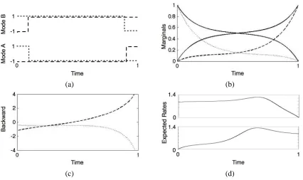
Example 3 Let us return to the two-component Ising chain in Example 1 with initial state X₁(0)=−1 and X₂(0)=1, and a reversed state at the final time, X₁(T)=1 and X₂(T)=−1. For a large value ofβ, this evidence is unlikely as at both end points the components are in a undesired configurations. The exact posterior is one that assigns higher probabilities to trajectories where one of the components switches relatively fast to match the other, and then toward the end of the interval, they separate to match the evidence. Since the model is symmetric, these trajectories are either ones in which

both components are most of the time in state −1, or ones where both are most of the time in

state 1 (Figure 3(a)). Due to symmetry, the marginal probability of each component is around

0.5 throughout most of the interval. The variational approximation cannot capture the dependency

between the two components, and thus converges to one of two local maxima, corresponding to the two potential subsets of trajectories (Figure 3(b)). Examining the value ofρi, we see that close to the end of the interval they bias the instantaneous rates significantly. For example, as t approaches 1, ρ1

1(t)/ρ1−1(t)approaches infinity and so does the instantaneous rateγ−11,1(t)/µ1−1(t), thereby forcing X1to switch to state 1 (Figure 3(c)).

This example also allows to examine the implications of modeling the posterior by inhomoge-neous Markov processes. In principle, we might have used as an approximation Markov processes with homogeneous rates, and conditioned on the evidence. To examine whether our approximation behaves in this manner, we notice that in the single component case we have

qx,y=

ρx(t)γx,y(t) ρy(t)µx(t)

,

which should be constant.

(a) (b)

(c) (d)

Figure 3: Numerical results for the two-component Ising chain described in Example 3 where the first component starts in state−1 and ends at time T=1 in state 1. The second component has the opposite behavior. (a) Two likely trajectories depicting the two modes of the model. (b) Exact (solid) and approximate (dashed/dotted) marginals µi₁(t). (c) The log ratio logρi₁(t)/ρi

−1(t). (d) The expected rates ˜q11,−1(t)and ˜q1−1,1(t)of component X1of the Ising chain in Example 1. We can notice that the averaged rates are highly non-constant, and so cannot be approximated well with a constant rate matrix.

changes in time, these rates change continuously, especially near the end of the time interval. This suggests that a piecewise homogeneous approximation cannot capture the dynamics without a loss in accuracy. As expected in a dynamic process, we can see in Figure 3(d) that the inhomogeneous transition rates are very erratic. In particular, the rates of X1 spike at the transition point selected by the mean field approximation. This can be interpreted as putting most of the weight of the distribution on trajectories which transition from state -1 to 1 at that point.

4.2 Optimization Procedure

IfQis irreducible, thenρi_xi and µi_xi are non-zero throughout the open interval(0,T). As a result, we can solve (17) to express γi_xi,yi as a function of µi andρi, thus eliminating it from (16) to get evolution equations solely in terms of µiandρi. Abstracting the details, we obtain a set of ODEs of the form

d dtρ

i_{(t) =α(ρ}i_(t),µ\i_{(t)) ρ}i_{(T) =given,}

d dtµ

whereαandβare defined by the right-hand side of the differential equations (16). Since the evo-lution ofρi does not depend on µi, we can integrate backward from time T to solve forρi. Then,

integrating forward from time 0, we compute µi. After performing a single iteration of

backward-forward integration, we obtain a solution that satisfies the fixed-point equation (16) for the i’th com-ponent (this is not surprising once we have identified our procedure to be a variation of a standard forward-backward algorithm for a single component). Such a solution will be a local maximum

of the functional w.r.t. to ηi _{(reaching a local minimum or a saddle point requires very specific}

initialization points).

This suggests that we can use the standard procedure of asynchronous updates, where we update each component in a round-robin fashion. Since each of these single-component updates converges in one backward-forward step, and since it reaches a local maximum, each step improves the value of the free energy over the previous one. As the free energy functional is bounded by the probability of the evidence, this procedure will always converge, and the rate of the free energy increase can be used to test for convergence.

Potentially, there can be many scheduling possibilities. In our implementation the update scheduling is simply random. A better choice would be to update the component which would maximally increase the value of the functional in that iteration. This idea is similar to the schedul-ing of Elidan et al. (2006), who approximate the change in the beliefs by boundschedul-ing the residuals of the messages, which give an approximation of the benefit of updating each component.

Another issue is the initialization of this procedure. Since the iteration on the i’th component depends on µ\i, we need to initialize µ by some legal assignment. To do so, we create a fictional rate matrix ˜Qifor each component and initialize µito be the posterior of the process given the evidence ei,0and ei,T. As a reasonable initial guess, we choose at random one of the conditional ratesQi|ui

using some random assignment uito determine the fictional rate matrix.

The general optimization procedure is summarized in the following algorithm: For each i, initialize µi using some legal marginal function.

while not converged do

1. Pick a component i∈ {1, . . . ,D}.

2. Updateρi(t)by solving theρibackward differential equation in (16).

3. Update µi(t)andγi(t)by solving the µiforward differential equation in (16) and using the algebraic equation in (17).

end

Algorithm 1: Mean field approximation in continuous-time Bayesian networks

4.3 Exploiting Continuous-Time Representation

To further save computations, we note that while standard integration methods involve only initial boundary conditions at t=0, the solution of µi is also known at t=T . Therefore, we stop the adaptive integration when µi(t)≈µi(T)and t is close enough to T . This modification reduces

the number of computed points significantly because the derivative of µi tends to grow near the

boundary, resulting in a smaller step size.

The adaptive solver selects different time points for the evaluation of each component. There-fore, updates ofηi_{require access to marginal density sets of neighboring components at time points} that differ from their evaluation points. To allow efficient interpolation, we use a piecewise linear

approximation ofηwhose boundary points are determined by the evaluation points that are chosen

by the adaptive integrator.

5. Perspectives and Related Work

Variational approximations for different types of continuous-time processes have been recently

proposed. Examples include systems with discrete hidden components (Opper and Sanguinetti,

2007); continuous-state processes (Archambeau et al., 2007); hybrid models involving both discrete and continuous-time components (Sanguinetti et al., 2009; Opper and Sanguinetti, 2010); and spa-tiotemporal processes (Ruttor and Opper, 2010; Dewar et al., 2010). All these models assume noisy observations in a finite number of time points. In this work we focus on structured discrete-state processes with noiseless evidence.

Our approach is motivated by results of Opper and Sanguinetti (2007) who developed a varia-tional principle for a related model. Their model is similar to an HMM, in which the hidden chain is a continuous-time Markov process and there are (noisy) observations at discrete points along the process. They describe a variational principle and discuss the form of the functional when the ap-proximation is a product of independent processes. There are two main differences between the setting of Opper and Sanguinetti and ours. First, we show how to exploit the structure of the target CTBN to reduce the complexity of the approximation. These simplifications imply that the update of the i’th process depends only on its Markov blanket in the CTBN, allowing us to develop effi-cient approximations for large models. Second, and more importantly, the structure of the evidence in our setting is quite different, as we assume deterministic evidence at the end of intervals. This setting typically leads to a posterior Markov process in which the instantaneous rates used by Opper and Sanguinetti diverge toward the end point—the rates of transition into the observed state go to infinity, leading to numerical problems at the end points. We circumvent this problem by using the marginal density representation which is much more stable numerically.

Taking the general perspective of Wainwright and Jordan (2008), the representation of the dis-tribution uses the natural sufficient statistics. In the case of a continuous-time Markov process, the sufficient statistics are Tx, the time spent in state x, and Mx,y, the number of transitions from state x to y. In a discrete-time model, we can capture the statistics for every random variable. In a continuous-time model, however, we need to consider the continuous-time derivative of the statistics. Indeed, as shown in Section 3.3 we have

d

dtE[Tx(t)] =µx(t) and d

dtE[Mx,y(t)] =γx,y(t).

Thus, our marginal density setsη provide what we consider a natural formulation for variational

Our presentation focused on evidence at two ends of an interval. Our formulation easily extends to deal with more elaborate types of evidence: (1) If we do not observe the initial state of the i’th component, we can set µi_x(0)to be the prior probability of X(0)=x. Similarly, if we do not observe Xi at time T , we setρi_x(T) =1 as initial data for the backward step. (2) In a CTBN where one (or more)

components are fully observed throughout some interval, we simply set µi for these components to

be a distribution that assigns all the probability mass to the observed trajectory. Similarly, if we observe different components at different times, we may update each component on a different time

interval. Consequently, maintaining for each component a marginal distribution µi throughout the

interval of interest, we can update the other ones using their evidence patterns.

6. Evaluation on Ising Chains

To gain better insight into the quality of our procedure, we performed numerical tests on models that challenge the approximation. Specifically, we use Ising chains with the parameterization in-troduced in Example 1, where we explore regimes defined by the degree of coupling between the

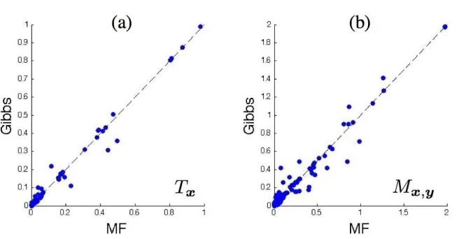
components (the parameterβ) and the rate of transitions (the parameterτ). We evaluate the error

in two ways. The first is by the difference between the true log-likelihood and our estimate. The second is by the average relative error in the estimate of different expected sufficient statistics de-fined by∑j|θjˆ −θj|/θj, whereθj is exact value of the j’th expected sufficient statistics and ˆθj is the approximation. To obtain a stable estimate the average is taken over allθj>0.05 maxj′θj′.

Applying our procedure on an Ising chain with 8 components, for which we can still perform

exact inference, we evaluated the relative error for different choices of βandτ. The evidence in

this experiment is e0={+,+,+,+,+,+,−,−}, T=0.64 and eT={−,−,−,+,+,+,+,+}. As

shown in Figure 4(a), the error is larger when τandβ are large. In the case of a weak coupling

(smallβ), the posterior is almost factored, and our approximation is accurate. In models with few

transitions (smallτ), most of the mass of the posterior is concentrated on a few canonical “types” of trajectories that can be captured by the approximation (as in Example 3). At high transition rates, the components tend to transition often, and in a coordinated manner, which leads to a posterior that is hard to approximate by a product distribution. Moreover, the resulting free energy landscape is rough with many local maxima. Examining the error in likelihood estimates (Figure 4(b),(c)) we see a similar trend.

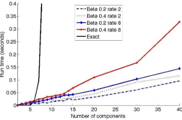
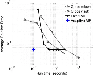
Next, we examine the run time of our approximation when using fairly standard ODE solver with few optimizations and tunings. The run time is dominated by the time needed to perform the backward-forward integration when updating a single component, and by the number of such

updates until convergence. Examining the run time for different choices ofβandτ(Figure 5), we

see that the run time of our procedure scales linearly with the number of components in the chain. The differences among the different curves suggest that the runtime is affected by the choice of parameters, which in turn affect the smoothness of the posterior density sets.

7. Evaluation on Branching Processes