Robust Process Discovery with Artificial Negative Events

Robust Process Discovery with Artificial Negative Events

Stijn Goedertier [email protected]

David Martens∗ [email protected]

Jan Vanthienen [email protected]

Bart Baesens† [email protected]

Faculty of Business and Economics Katholieke Universiteit Leuven Leuven, Naamesestraat 69, Belgium

Editor: Paolo Frasconi, Kristian Kersting, Hannu Toivonen and Koji Tsuda

Abstract

Process discovery is the automated construction of structured process models from information sys-tem event logs. Such event logs often contain positive examples only. Without negative examples, it is a challenge to strike the right balance between recall and specificity, and to deal with problems such as expressiveness, noise, incomplete event logs, or the inclusion of prior knowledge. In this paper, we present a configurable technique that deals with these challenges by representing process discovery as a multi-relational classification problem on event logs supplemented with Artificially Generated Negative Events (AGNEs). This problem formulation allows using learning algorithms and evaluation techniques that are well-know in the machine learning community. Moreover, it allows users to have a declarative control over the inductive bias and language bias.

Keywords: graph pattern discovery, inductive logic programming, Petri net, process discovery,

positive data only

1. Introduction

Learning descriptive or predictive models from sequence data is an important data mining task with applications in Web usage mining, fraud detection, bio-informatics, and process discovery. The learning task can be formulated as follows: given a sequence database that contains a finite number of sequences, find a useful generative model that describes or predicts its spatio-temporal properties. Depending on the application domain, a variety of sequence models and corresponding learning algorithms are available. For instance, probabilistic generative models such as (hidden) Markov models have been successfully applied in speech analysis, and bio-informatics (Durbin et al., 1998), whereas deterministic models such as partial orders have been applied in domains such as Web usage mining (Mannila and Meek, 2000; Pei et al., 2006). In this paper, we focus on the problem of process discovery, the discovery of business process models from event-based data generated by information systems. Process models typically contain structures such as sequences, or-splits, and-splits (parallel threads), or-joins, and-joins, loops (iterations), non-local, non-free, history-dependent or-splits, and duplicate activities. Because Petri nets can represent these

con-∗. David Martens is also at the Department of Business Administration and Public Management, University College

Ghent, Association Ghent University, Belgium.

structs, they are known to be a convenient process modeling language (van der Aalst, 1998; Alves de Medeiros, 2006) provides a detailed overview of how these structures can be represented with Petri nets.

The motivation for process discovery is the abundant availability of information system event logs. The analysis of such event logs can provide insight into how processes actually take place, and to what extent actual processes deviate from a normative process model. Information system events keep track of, among others, the completion of an activity of a particular activity type. For example, an event can report that a particular activity of type ‘apply for license’ has completed. The goal of process discovery is to construct a useful process model that describes the event sequences recorded in the event log. Example 1, illustrates the learning problem for a fictitious driver’s license application process. Given the event sequence database in Example 1, a useful process models is to be conceived.

Example 1 DriversLicensel—discovery of a driver’s license application process with loop. The transitions correspond to activity types that have the following meaning: a start, b apply for li-cense, c attend classes cars, d attend classes motor bikes, e obtain insurance, f theoretical exam, g practical exam cars, h practical exam motor bikes, i get result, j receive license, and k end.

σ1 abcefgijk

σ2 abdfehijk

σ3 abdefhijbdfehijk

σ4 abcfegik

. . . .

a b c d e f

g h i j

k b

b c d

g h f

i e

a

k k j

(a) sequences (b) general (c) specific and general

d d

a a a a

b b b b

c c

f

f f

f

e e

e e

k k k k

... ... ... ...

(d) over-specific

The construction of useful process models from an event log is subjected to many challenging problems. An inherent difficulty is that process discovery is limited to a setting of unsupervised learning. Event logs rarely contain negative information about state transitions that were prevented from taking place. Such negative information can be useful to discover the discriminating properties of the underlying process. In the absence of negative information, it is necessary to provide a learner with a particular inductive bias, to accurately strike the right balance between generality and speci-ficity. The absence of negative information, makes the learning task aim at accurately summarizing an event log such that the discovered process model allows the observed behavior (recall) but does not include unintended, random behavior that is not present in the event log (specificity). In addition to accuracy, the learning problem faces challenges such as expressiveness, noise, incomplete event logs, and the inclusion of prior knowledge:

Example 1, called a flower model, is capable of parsing every sequence in the event log. How-ever, it can be considered to be overly general as it allows any activity to occur in any order. In contrast, the Petri net in Example 1 is overly specific, as it provides a mere enumeration of the different sequences in the event log. The Petri net in Example 1 is likely to be the more suitable process model. It is well-structured, and strikes a reasonable balance between specificity and generality, allowing for instance an unseen sequence abcefgik, but disallowing random behavior. An additional difficulty is that in the absence of negative information, the specificity of a learned process model is difficult to quantify.

• expressiveness: expressiveness relates to the ability to comprehensively summarize an event log using a rich palette of structures such as sequences, or-splits, and-splits (parallel threads), or-joins, and-joins, loops (iterations), history-dependent or-splits, and duplicate activities.

• noise: human-centric processes are prone to exceptions and logging errors. This causes ad-ditional low-frequent behavior to be present in the event log that is unwanted in the process model to be learned. Process discovery algorithms face the challenge of not overfitting this noise.

• incomplete logs: incomplete event logs do not contain the complete set of sequences that occur according to the underlying, real-life process. This is particularly the case for pro-cesses that portray a large amount of concurrent and recurrent behavior. In this case, process discovery algorithms must be capable of generalizing beyond the observed behavior.

• prior knowledge: the problem of consolidating the knowledge extracted from the data with the knowledge representing the experience of domain experts, is called the knowledge fusion problem (Dybowski et al., 2003). Prior knowledge constrains the hypothesis space of a se-quence mining algorithm. In the context of process discovery, prior knowledge might refer to knowledge about concurrency (parallelism), locality, or exclusivity of activities. When a learner produces a process model that is not in line with the prior knowledge of a domain expert, the expert might refuse using the discovered process model. For instance, a domain expert might refuse a process model in which a pair of activities cannot take place concur-rently, whereas in reality such parallelism is actually allowed.

In this paper, these challenges addressed by representing process discovery as an ILP classi-fication learning problem on event logs supplemented with artificially generated negative events (AGNEs). The AGNEs technique is capable of constructing Petri net models from event logs and has been implemented as a mining plugin in the ProM framework. A benchmark experiment with 34 artificial event logs and comparison to four state-of-the-art process discovery algorithms indicate that the technique is expressive, robust to noise, and capable of dealing with incomplete event logs. A second contribution of the paper is the definition of a new metric for quantifying the specificity of an induced process model, based on these artificially generated negative events.

2. Preliminaries

This section introduces the most important concepts and notations that are used in the remainder of this paper.

2.1 Inductive Logic Programming

Inductive Logic Programming (ILP) (Muggleton, 1990; Dˇzeroski and Lavraˇc, 1994, 2001; Dˇzeroski, 2003) is a research domain in machine learning involving learners that use logic programming to represent data, background knowledge, the hypothesis space, and the learned hypothesis. ILP learners are called multi-relational learners and extend classical, uni-relational learners in the sense that they can not only learn patterns that occur within single tuples (within rows), but can also find patterns that may range over different tuples of different relations (between multiple rows of a single or multiple tables). For process discovery, this multi-relational property is much desired, as it allows discovering patterns that relate the occurrence of an event to the occurrence of any other event in the event log.

Within ILP, concept learning is an important learning task. An ILP classification learner will search for a hypothesis H in a hypothesis space S_{that best discriminates between the positive P}

and negative examples N (E=P∪N) in combination with some given background knowledge B. A particularly salient feature of such learners is that they have a highly configurable language bias. The language biasL_{specifies the hypothesis space}S_{of logic programs H that can be considered.}

In addition, users of ILP learners can specify background knowledge B as a logic program. Such background knowledge is a more parsimonious encoding of knowledge that is true about every example, than is the case for the attribute-value encoding of propositional learners. In addition to their multi-relational capabilities, the power of ILP concept learners lies with the configurability of their language biasL_{and background knowledge B. The effectiveness by which an ILP learner can}

be applied to a learning task depends on the choices that are made in representing the examples E, the background knowledge B and the language biasL_.

In this text, we make use of TILDE (Blockeel and De Raedt, 1998), a first-order decision tree learner available in the ACE-ilProlog data mining system (Blockeel et al., 2002). Blockeel (1998) formalizes the learning task of TILDE as follows:

given:

• a set of classes C

• a set of classified examples E, each example(e,c)∈E is an independent logic program for which the predicate Class(c)denotes that e is classified into class c.

• a logic program B that represents the background knowledge

• a language biasL_{that specifies a hypothesis space}S_{of logic programs.}

find: a hypothesis H∈S_{(a logic program) such that for all labeled examples(e,c)∈E,}

• ∀e∈E : H∧e∧BClass(c)

TILDE is a first-order generalization of the well-known C4.5 algorithm for decision tree induc-tion (Quinlan, 1993). Like C4.5, TILDE (Blockeel and De Raedt, 1998; Blockeel et al., 2002) ob-tains classification rules by recursively partitioning the data set according to logical conditions that can be represented as nodes in a tree. This top-down induction of logical decision trees (TILDE) is driven by refining the node criteria according to the provided language biasL_{. Unlike C4.5, TILDE}

is capable of inducing first-order logical decision trees (FOLDT). A FOLDT is a tree that holds logical formula containing variables instead of propositions. Blockeel and De Raedt (1998) show how each FOLDT can be converted into a logic program.

2.2 Event Logs

In process discovery, an event log is a database of event sequences. Each event reports an instan-taneous state change of an activity of a particular activity type. Activities and events that pertain to the same process instance are identified by a so-called case identifier. In process discovery, the MXML format for event logs (van Dongen and van der Aalst, 2005a) is the commonly accepted format for event logs. To use event logs with TILDE event logs have to be represented as a logi-cal program. Let X be a set of event identifiers, P a set of case identifiers, the alphabet A a set of activity types, and E={completed,completeRejected}a set of event types. An event predicate is a quintuple Event(x,p,a,e,t), where x∈X is the event identifier, p∈P is the case identifier, a∈A the activity type, e∈E the event type, and t∈Nthe time of occurrence of the event. The function Case∈X∪L→P denotes the case identifier of an event or a sequence. The function AT∈X→A denotes the activity type of an event. The function ET∈X→E denotes the event type of an event. The function Time∈X→Ndenotes the time of occurrence of an event. The set X of identifiers has a complete ordering, such that∀x,y∈X : x<y∨y<x and∀x,y∈L : x<y⇒Time(x)≤Time(y). The event types E={completed,completeRejected}respectively indicate the completion of a particular activity or that the completion of a particular activity could not take place, a negative event.

Let an event log L be a set of sequences σ. Letσ∈L be an event sequence, an ordered set of event identifiers x∈X of events pertaining to the same process instance as denoted by the case id; σ={x|x∈X∧Case(x) =Case(σ)}. The function Position∈X×L→N0 denotes the position of an event with identifier x∈X in the sequenceσ∈L. Two subsequent event identifiers within a sequenceσcan be represented as a sequence x.y⊆σ. We define the .-predicate as follows

x.y⇔ ∃x,y∈σ: x<y∧∄z∈σ: x<z<y.

In the text, this predicate is used within the context of a single sequenceσwhich is therefore left implicit. Given that AT(x) =a,AT(y) =b the information in the sequence can be further abbreviated as ab, because the order of the activity types in a sequence is the most important information for the purpose of process discovery. This notation is used to represent the event log in Example 1. Each rowσi in the event log represents a different execution sequence that corresponds to a particular process instance.

2.3 Petri Nets

Each different distribution of tokens over the places of a Petri net indicate a different state. Such a state is called a marking. Transitions (drawn as rectangles) can consume and produce tokens and represent a state change. Arcs (drawn as arrows) connect places and transitions and represent a flow relationship. More formally, a marked Petri net is a pair((P,T,F),s)where,

• P is a finite set of places,

• T is a finite set of transitions such that P∩T =/0, and

• F⊆(P×T)∪(T×P)is a finite set of direct arcs, and

• s∈P→Nis a bag over P denoting the marking of the net (van der Aalst, 1997, 1998).

Petri nets are bipartite directed graphs, that means that each arc must connect a transition to a place or a place to a transition. The transitions in a Petri net can be labeled or not. Transitions that are not labeled are called silent transitions. Different transitions that bear the same label are called duplicate transitions.

The behavior of a Petri net is determined by the firing rule. A transition t is enabled iff each input place p of t contains at least one token. When a transition is enabled it can fire. When a transition fires, it brings about a state change in the Petri net. In essence, it consumes one token from each input place p and produces one token in each output place p of t. To evaluate the extent to which a Petri net is capable of parsing an event sequence, transitions might be forced to fire. A transition that is not enabled, can be forced to fire. When a transition is forced to fire, it consumes one token from each input place that contains a token—if any—and produces one token in each output place. Petri nets are capable of representing structures such as sequences, or-splits, and-splits (parallel threads), or-joins, and-joins, loops (iterations), history-dependent or-splits, and duplicate activities that are typical for organizational processes.

3. Artificial Negative Events

Event logs generally contain sequences of positive events only. To make a tradeoff between overly general or overly specific process models, learners make additional assumptions about the given event sequences. Such assumptions are part of the inductive bias of a learner. Process discovery algorithms generally include the assumption that event logs portray the complete behavior of the underlying process and implicitly use this completeness assumption to make a tradeoff between overly general and overly specific process models. Our technique makes this completeness assump-tion explicit by inducing artificial negative informaassump-tion from the event log in a configurable way.

For processes that contain a lot of recurrent and concurrent behavior, the completeness assump-tion can become problematic. For example, a process containing five parallel activities (ten parallel pairs) that are placed in a loop, has∑n_i=1(5!)i _{different possible execution sequences (n being the} maximum number of allowed loops).

of loops (recurrent behavior) in the underlying process. Limiting the window size to a smaller sub-sequence of the event log, makes the completeness assumption less strict. An unlimited window size (windowSize=−1) results in the most strict completeness assumption.

The problem of concurrent behavior is addressed by exploiting some available parallelism in-formation, discovered by induction or provided as prior knowledge by a domain expert. Given a subsequence and parallelism information, all parallel variants of the subsequence can be calculated. Taking into account the parallel variants of a subsequence makes the completeness assumption less strict.The function AllParallelVariants(τ)returns the set of all parallel variants that can be obtained by permuting the activities in each sub-sequence ofτwhile preserving potential dependency rela-tionships among non-parallel activities.

Negative events record that at a particular position in an event sequence, a particular event cannot occur. At each position k in each event sequenceτi, it is examined which negative events can be induced for this position. Algorithm 1 gives an overview of the negative event induction and is discussed in the next paragraphs. In a first step, the event log is made more compact, by grouping process instances σ∈L that have identical sequences into grouped process instances τ∈M (line 1). By grouping similar process instances, searching for similar behavior in the event log can be performed more efficiently.

In the next step, all negative events are induced for each grouped process instance (lines 2–12). Making a completeness assumption about an event log boils down to assuming that behavior that does not occur in the event log, should not occur in the process model to be learned. Negative examples can be introduced in grouped process instancesτiby checking at any given positive event xk ∈τi at position k=Position(xk,τi) whether another event of interest zk of activity type b∈ A\{AT(xk)} also could occur. For each event xk ∈τi, it is tested whether there exists a similar sequenceτk_j∈AllParallelVariants(τj):τj6=τiin the event log in which at that point a state transition yk has taken place that is similar to zk(line 6). If such a state transition does not occur in any other sequence, such behavior is not present in the event log L. This means under the completeness assumption that the state transition cannot occur. Consequently, zk can be added as a negative event at this point k in the event sequenceτi(lines 7–8). On the other hand, if a similar sequence is found with this behavior, no negative event is generated.

Finally, the negative events in the grouped process instances are used to induce negative events into the similar non-grouped sequences. If a grouped sequenceτcontains negative events at position k, then the ungrouped sequence σcontains corresponding negative events at position k. At each position, a large number of negative events can generally be generated. To avoid an imbalance in the proportion of negative versus positive events the addition of negative events can be manipulated with a negative event injection probabilityπ(line 13).πis a parameter that influences the probability that a corresponding negative event is recorded in an ungrouped traceσ. The smallerπ, the less negative events are generated at each position in the ungrouped event sequences. A value ofπ=1.0 means that every induced negative event for a grouped sequence is included in every similar, corresponding, non-grouped sequence. A value ofπ=0 will result in no negative events being induced for any of the corresponding, non-grouped sequences.

Example 2 illustrates how in an event log of two (grouped) sequencesτ1andτ2artificial negative

events can be generated. The event sequences originate from a simplified driver’s license process, depicted at the bottom. Given the parallelism information, Parallel(e,f), the event sequences each have two parallel variants. When generating negative events into event sequenceτ1, it is examined

Algorithm 1 Generating artificial negative events

1: Group similar sequencesσ∈L intoτ∈M

2: for allτi∈M do

3: for all xk∈τido

4: k=Position(xk,τi)

5: for all b∈A\{AT(xk)}do

6: if∄τk_j ∈AllParallelVariants(τj):∀τj∈M∧τj6=τi∧

∀yl ∈ τkj,Position(yl,τkj) = l = Position(xl,τj),k−windowSize < l < k : AT(yl) = AT(xl)∧

yk∈τkj,Position(yk,τkj) =k,AT(yk) =b then

7: zk= event with AT(zk) =b,ET(zk) =completeRejected

8: recordNegativeEvent(zk,k,τi)

9: end if

10: end for

11: end for

12: end for

13: Induce negative events in the non-grouped sequencesσ∈L according to an injection frequency π

first position. Because there is no similar sequence τk_j in which c,d,e,f,g,h,or i occur at this position, it can be concluded that they are negative events. Consequently ¬c,¬d,¬e,¬f,¬g,¬h,

and¬i are added as negative events at this position. Other artificial negative events are generated in a similar fashion. Notice that history-dependent processes generally will require a larger window size to correctly detect all non-local dependencies. In Example 2, an unlimited window size is used. Should the window size be limited to 1, for instance, then it would no longer be possible to take into account the non-local dependency between the activity pairs c–g and d–h. In the experiments at the end of this paper, an unlimited window size has been used (parameter value -1).

4. Process Discovery

Having an algorithm to artificially generate negative events, it becomes possible to represent process discovery as a binary classification problem, that learns the conditions that discriminate between the occurrence of an activity (a positive event), or the non-occurrence of an activity (a negative event). Algorithm 2 outlines four major steps in the AGNEs process discovery procedure. These four steps are addressed this section.

4.1 Step 1: Induce Parallelism and Locality Information

Example 2 (Continued from example 1.) DriversLicense—Generating artificial negative events for a simplified event log with two abbreviated event sequences.

τ1 b c e f g i

τ2 b d f e h i

Parallel(e,f).

(a) given event log and background knowledge

τk

1 b c f e g i

τk

1 b c e f g i

τk

2 b d f e h i

τk

2 b d e f h i

(b) the derived parallel variants

τ1 b c e f g i

¬c ¬b ¬b ¬b ¬b ¬b

¬d ¬e ¬c ¬c ¬c ¬c

¬e ¬f ¬d ¬d ¬d ¬d

¬f ¬g ¬g ¬g ¬e ¬e

¬g ¬h ¬h ¬h ¬f ¬f

¬h ¬i ¬i ¬i ¬h ¬g

¬i ¬i ¬h

τ2 b d f e h i

¬c ¬b ¬b ¬b ¬b ¬b

¬d ¬e ¬c ¬c ¬c ¬c

¬e ¬f ¬d ¬d ¬d ¬d

¬f ¬g ¬g ¬g ¬e ¬e

¬g ¬h ¬h ¬h ¬f ¬f

¬h ¬i ¬i ¬i ¬g ¬g

¬i ¬i ¬h

(c) the induced negative events

b c

d

g h

f i

e

(d) the underlying Petri net

Algorithm 2 Process discovery by AGNEs: overview

1: step 1: induce parallelism and locality from frequent temporal constraints

2: step 2: generate artificial negative events

3: step 3: learn the preconditions of each activity type

4: step 4: transform the preconditions into a Petri net

that cannot easily be transformed into a graphical model. Parallelism information is used to prevent the construction of sequential models, where in reality concurrency is expected.

This information is either gathered by the analysis of frequent temporal constraints that hold in the event log or by means of user-specified prior knowledge. Frequent temporal constraints are temporal constraints that hold in a sufficient number of sequences σ within an event log L. Goedertier (2008), defines a number of temporal constraints and shows how local dependency and parallelism information can be derived from it.

Additionally, the end-user can also specify locality and parallelism information in terms of prior knowledge. In particular, the following predicates can be used: PriorParallel(a,b), PriorSerial(a,b), PriorLocal(a,b), and PriorNonLocal(a,b). Information specified using these predicates defeats any inference about locality or parallelism made on the basis of the information gathered from frequent temporal constraints.

4.2 Step 2: Generate Artificial Negative Events

variant calculation. Furthermore, the induction of negative events is dependent on the window size windowSize, and negative event injection probabilityπparameters.

4.3 Step 3: Learn the Preconditions of each Activity Type

It is now possible to represent process discovery as a multiple, first-order classification learning problem that learns the preconditions that discriminate between the occurrence of either a positive or a negative completion event for each activity type. In our experiments, we make use of TILDE, an existing multi-relational classification learner, to perform the actual classification learning.

The motivation for representing process discovery as a classification problem is that it allows using classification learning and evaluation techniques that are well-known in the machine learning community. Furthermore, classification learners have the potential to deal with so-called duplicate tasks. Duplicate tasks refer to the reoccurrence of identically labeled transitions, homonyms, in different contexts within the event logs. Classification learning can detect the different execution contexts for these transitions and derive different preconditions for them. Transforming these pre-conditions into graphs will eventually result in duplicate, homonymic activities in the graph model that correspond to the different usage contexts. Techniques for process discovery, such as heuris-tics miner and genetic miner, which have causal matrices as internal representation (Weijters et al., 2006; Alves de Medeiros et al., 2007), are unable to discover duplicate activities. Alves de Medeiros (2006), however, presents a non-trivial extension of the genetic miner that includes duplicate tasks. The motivation for using a multi-relational, first-order representation is that first-order learning allows relating the occurrence of an event to the occurrence of any other event. This enables the detection of patterns that involve non-local, historic, dependencies between events. Alternatively, the history of each event could in part be represented as extra propositions, for instance by including all preceding positive events as extra columns in the event log. This propositional representation would have many difficulties.

Being able to detect non-local, historic patterns in an event log can also produce counter-intuitive results. A non-local relationship might have more discriminating power than a local one and can therefore be preferred by a learner. Unfortunately, an excess of non-local patterns makes it more difficult to generate a graphical model, a Petri net, containing local connections. Because TILDE al-lows specifying a language bias with dynamic refinement (Blockeel and De Raedt, 1998), it becomes possible to constrain the hypothesis space to locally discriminating patterns whenever necessary. One technique is the dynamic generation of constants, that can be used to constrain the combina-tions of activity type constants that are to be considered for a particular language bias construct. Additionally, it is also possible to constrain the occurrence of particular literals in a hypothesisH_,

given the presence or absence of other literals that are already part of the hypothesis.

The classification task of TILDE is to predict whether for a given activity type a∈A, at a given time point t ∈N in a given sequence σ∈L, a positive or a negative event takes place. In the case of a positive event, the target predicate evaluates to Class(a,σ,t,completed). In the case of a negative event, the target predicate evaluates to Class(a,σ,t,completeRejected). In the language bias, the target activity, indicated by a, will be used for dynamically constraining the combinations of activity type constants generated.

a1,a∈A be activity types,σ∈L the sequence of a process instance, and t the time of observation.

The NS predicate is defined as follows:

∀a1,a∈A,t∈N:∃x∈σ: AT(x) =a1 ∧ Time(x)<t

∧∄y∈σ: AT(y) =a ∧ Time(x)<Time(y)<t ⇒NS(a1,a,σ,t).

In the remainder of this text, the argumentsσand t will be implicitly assumed and therefore left out. The predicate NS(a1,a) evaluates to true when at the time of observation, an activity a1 has

completed, but has not (yet) been followed by an activity a. In combination with conjunction (∧), disjunction (∨) and negation-as-failure (∼), the NS(a1,a)predicate makes it possible to learn

frag-ments of Petri nets using a multi-relational classification learner.

Example 3 shows how the preconditions in the Petri net can be represented as conjunctions and disjunctions of NS atoms. This representation accounts for the different contexts in which the activ-ities applyForLicense and end can take place and derives different preconditions for these activactiv-ities. In addition, it can represent the non-local, non-free, history-dependent choice construct between the

activities attendClassesCars–doPracticalExamCars and attendClassesMotorBikes–

doPracticalExamMotorBikes and the maximum recurrence of the activity applyForLicense. The Petri net fragments included in the language bias of AGNEs are enumerated in Figure 1 and are briefly discussed in the remainder of this section.

Example 3 (Continued from example 2) DriversLicensel—A Petri net in terms of NS preconditions

activity precondition

a start true

b applyForLicense NS(a,b)

b applyForLicense (NS(i,b)∧NS(i,j)∧NS(i,k)) ∧OccursLessThan(b,3) c attendClassesCars NS(b,c)∧NS(b,d) d attendClassesMotorBikes NS(b,c)∧NS(b,d) e obtainInsurance NS(c,e)∨NS(d,e) f doTheoreticalExam NS(c,f)∨NS(d,f) g doPracticalExamCars (NS(f,g)∧NS(f,h))∧

(NS(e,g)∧NS(e,h))∧NS(c,g)

h doPracticalExamMtrBikes (NS(f,g)∧NS(f,h))∧

(NS(e,g)∧NS(e,h))∧NS(d,h)

i getResult NS(g,i)∨NS(h,i) j receiveLicense NS(i,b)∧NS(i,j)∧NS(i,k)

k end NS(j,k)

k end NS(i,b)∧NS(i,j)∧NS(i,k)

applyF orLicense applyF orLicense

[OccursLessT han(applyF orLicense,3)]

[OccursLessT han(applyF orLicense,3)]

attendClassesCars attendClassesM otorBikes

doP racticalExamCars doP racticalExamM otorBikes doT heoreticalExam

getResult obtainInsurance

start

receiveLicense end

end

(a) DriversLicensel—activity preconditions (b) DriversLicensel—Petri net

Figure 1(a) shows a graphical representation of the local sequence predicate that is part of the language bias. A local sequence of two transitions labeled a1,a∈A in a Petri net can be represented

a1 a

NS(a1,a)

(a) local sequence

a

[OccursLessT han(a, N)]

OccursLessThan(a,N)

(b) max occurrence

a

[:Attribute=V alue]

: Attribute=Value

(c) data condition

a1

a2

a

NS(a1,a)∧NS(a1,a2)

(d) or-split

a1 a

NS(a1,a)

(e) global sequence

a1

a2

a

NS(a1,a)∨NS(a2,a)

(f) or-join

a1 a2

a

NS(a1,a)∧NS(a1,a2)

(g) skip sequence

Figure 1: Petri net patterns in the language bias

sequence NS(a1,a)

constraints: Local(a1,a). (1)

∄l∈H: l= [NS(,a1)]. (2)

The conversion from NS-based preconditions into Petri nets requires the conditions to refer to lo-cal, immediately preceding events as much as possible. Therefore, constraint (1) requires to restrict the generation of constants a1to constants that are local to a. In constraint (1) we do not require a1

and a to be different activity types. This is sufficient for the discovery of length-one loops. Graphi-cally, a conjunction of NS constructs can be considered to be the logical counterpart of a single Petri net place. Besides the case of length-one loops—that can be expressed with a single NS construct— there is no reason for a Petri net place to contain both an input and an output arc that is connected to the same transition. Constraint (2) has been put in place to keep a multi-relational learner from constructing such useless hypotheses. The constraint stipulates that the construct NS(a1,a)can only

be added to the current hypothesisH_{, if}H_{does not already contain a logical condition that boils}

down to an output arc towards a1.

The same NS(a1,a)construct, with different constraints, can be used to keep track of a global

The language bias of TILDE is limited to conjunctions and disjunctions of NS constructs of length two and three. Or-splits and or-joins that involve more activity types are obtained by grouping conjunctions and disjunctions of NS constructs into larger conjunctions and disjunctions in step 4. However, this limitation in length sometimes leads to TILDE make inadequate refinements. Solving this language bias issue, requires constructing a proprietary ILP classification algorithm that during each refinement step allows considering conjunctions of NS constructs of variable lengths. We leave this improvements to future work.

4.4 Step 4: Transform the Preconditions into a Petri Net

In the previous step, TILDE has learned preconditions for each activity type independently. In a Petri net, the preconditions for each activity type are nonetheless interrelated. Therefore, the logic programs of activity preconditions are submitted to several rule-level pruning steps, to make sure that they do not produce redundant duplicate places in the Petri net to be constructed. These pruning steps occur among the conditions within a single precondition, within a set of preconditions to the same activity type and among preconditions of activity types that pertain to the same or-split. Given a pruned rule set of preconditions for each activity type, the construction of a Petri net is fairly straightforward. Each induced precondition corresponds to a different transition in a Petri net to be constructed. Because AGNEs may produce several preconditions for an activity type, the constructed Petri net may contain duplicate transitions. Algorithm 3 provides an overview of these procedures. In the remainder of this section, these different pruning steps will be discussed and illustrated for a sample of rules from the DriversLicensel example.

The logic programs constructed by TILDE contain rules that classify the occurrence of either a positive or a negative event. By construction, the language bias of AGNEs is such that TILDE will never consider a negation of an NS construct to be explanatory for the occurrence of a positive event. Therefore, TILDE will never construct a tree in which a right leaf predicts a positive event. The latter entails that, in equivalent the logic program, the rules with a class(a,σ,t,comleted)rule head can be taken from the logic programs without loss of information (line 1). Example 4 depicts the preconditions that are induced by TILDE for the apply for license and end activities in the DriversLicensel example.

In a second step, a number of intra-rule pruning operations take place (lines 2–6). The top-down refinement of hypotheses, can result in the derivation of logically redundant conditions. These logical redundancies are removed for each rule (line 3). Each rule in the logic program consists of conjunctions of groups of NS constructs. A conjunction of a pair of or-split constructs that originate from the same activity a1 can be combined into a larger or-split (line 4). Likewise, a conjunction

of a pair of or-joins can be combined into a larger or-join (line 5). Example 4 illustrates intra-rule pruning for the DriversLicensel example.

Example 4 (Continued from example 3.) DriversLicensel—pruning

rules induced by TILDE :

b apply for license (NS(i,b)∨NS(a,b))∧(NS(i,b)∧NS(i,j)).

b apply for license (NS(i,b)∨NS(a,b)).

k end (NS(j,k)).

k end (NS(i,b)∧NS(i,k)).

intra-rule pruning:

b apply for license (NS(i,b)∧NS(i,j)).(line 3)

b apply for license (NS(i,b)∨NS(a,b)).

k end (NS(j,k)).

k end (NS(i,b)∧NS(i,k)).

inter-rule pruning, most specific or split:

b apply for license (NS(i,b)∧NS(i,j)∧NS(i,k)).(lines 18–26)

b apply for license (NS(a,b)).(lines 10–12)

k end (NS(j,k)).

k end (NS(i,b)∧NS(i,j)∧NS(i,k)).(lines 18–26)

5. Evaluation Metrics

Discovered process models preferably allow the behavior in the event log (recall) but no other, unobserved, random behavior (specificity). Having formulated process discovery as a binary classi-fication problem on event logs supplemented with artificial negative events, it becomes possible to use the true positive and true negative rate from classification learning theory to quantify the recall and specificity of a process model:

• true positive rate TPrate or recall: the percentage of correctly classified positive events in the event log. This probability can be estimated as follows: TPrate= TP

TP+FN, where TP is the amount of correctly classified positive events and FN is the amount of incorrectly classified positive events.

• true negative rate TNrateor specificity: the percentage of correctly classified negative events in the event log. This probability can be estimated as follows: TNrate= _TNTN_+FP, where TN is the amount of correctly classified negative events and FP is the amount of incorrectly classified negative events.

Accuracy is the sum of the true positive and true negative rate, weighted by the respective class distributions. The fact that accuracy is relative to the underlying class distributions can lead to unintuitive interpretations. Moreover, in process discovery, these class distributions can be quite different and have no particular meaning. In order to make abstraction of the proportion of negative and positive events, we propose, from a practical viewpoint to attach equal importance to both recall and specificity: acc= 1

2recall+ 1

2specificity. According to this definition, the accuracy of

a majority-class predictor is 1₂. Flower models, such as the one in Example 1(b), are an example of such a majority-class predictors. Because a flower model represents random behavior, it has a perfect recall of the all behavior in the event log but it also has much additional behavior compared to the event log. Because of the latter fact, the flower model has zero specificity, and an accuracy of

1

Algorithm 3 Rule-level pruning

1: R+={r∈R|r has rule head class(a,σ,t,comleted)}. // intra-rule pruning:

2: for all r∈R+do

3: reduce r according to(NS1∨NS2)∧NS1≡NS1.

4: group or-splits: NS(a1,a)∧NS(a1,a2) ∈r and NS(a1,a)∧NS(a1,a3) ∈r into NS(a1,a)∧

NS(a1,a2)∧NS(a1,a3).

5: group or-joins: NS(a1,a)∨NS(a2,a) ∈ r and NS(a3,a)∨NS(a4,a) ∈r into NS(a1,a)∨

NS(a2,a)∨NS(a3,a)∨NS(a4,a).

6: end for

//inter-rule pruning:

7: for all a∈A do

8: R+_a ={r∈R+|r is a precondition of a}

9: for all r∈R+_a do

10: if∃s∈R+_a : s is more specific than r then

11: remove r.

12: end if

13: if∃s∈R+_a : s combined with r lead to a more specific or-join than r then

14: replace the or-join in r with the more specific or-join.

15: end if

16: end for

17: end for

//keep the most specific or-split:

18: for all a∈A do

19: Rsplita ={r∈R+|r contains an or-split going out a}.

20: s = the most specific or-split by combining the or-splits going out a in Rsplita .

21: for all r∈Rsplita do

22: if s is more specific than r then

23: replace the or-split in r with the or-split in s.

24: end if

25: end for

26: end for

The metrics that are introduced in this section will be used to evaluate the performance of AGNEs in the following sections. They have been defined and implemented for Petri nets. However, they can also be applied to other generative models.

5.1 Existing Metrics

Weijters et al. (2006) define a metric that has a somewhat similar interpretation as TPrate: the parsing measure PM. The measure is defined as follows:

sequences, ni the number of process instances in a grouped sequence i, ci a variable that is equal to 1 if grouped sequence i can be parsed correctly, and 0 if grouped sequence i cannot be parsed correctly. The parsing measure can be defined as follows Weijters et al. (2006):

PM=∑

k i=1nici ∑k

i=1ni

.

PM is a coarse-grained metric. A single missing arc in a Petri net can result in parsing failure for all sequences. A process model with a single point of failure is generally better than a process model with more points of failure. This is not quantified by the parsing measure PM.

Rozinat and van der Aalst (2008) define two metrics that have a somewhat similar interpretation as TPrateand TNrate: the fitness metric f and the advanced behavioral appropriateness metric a′_B:

• fitness f : Fitness is a metric that is obtained by trying whether each (grouped) sequence in the event log can be reproduced by the generative model. This procedure is called sequence replay. The metric assumes the generative model to be a Petri net. At the start of the sequence replay, f has an initial value of one. During replay, the transitions in the Petri net will produce and consume tokens to reflect the state transitions. However, the proportion of tokens that must additionally be created in the marked Petri net, so as to force a transition to fire, is subtracted from this initial value. Likewise, the fitness measure f punishes for extra behavior by subtracting the proportion of remaining tokens relative to the total number of produced tokens from this initial value. Let k represent the number of grouped sequences, nithe number of process instances, ci the number of tokens consumed, mithe number of missing tokens, pi the number of produced tokens, and ri the number of remaining tokens for each grouped sequence i(1≤i≤k). The fitness metric can be defined as follows (Rozinat and van der Aalst, 2008):

f =1

2

1−∑

k i=1nimi ∑k

i=1nici

+1

2

1−∑

k i=1niri ∑k

i=1nipi

.

• behavioral appropriateness a′_B: Behavioral appropriateness is a metric that is obtained by an exploration of the state space of a Petri net and by comparing the different types of follows and precedes relationships that occur in the state space with the different types of follows and precedes relationships that occur in the event log. The metric is defined as the proportion of number of follows and precedes relationships that the Petri net has in common with the event log vis-`a-vis the number of relationships allowed by the Petri net. Let Sm_F be the SF relation and Sm_P be the SPrelation for the process model, and Sl_F the SF relation and Sl_Pthe SPrelation for the event log. The advanced behavioral appropriateness metric a′_B is defined as follows (Rozinat and van der Aalst, 2008):

a′_B=

|Sl_F∩S_Fm|

2.|Sm_F| +

|Sl_P∩Sm_P|

2.|Sm_P|

.

of invisible tasks such that the right activities become enabled for the Petri net to optimally replay a given sequence of events. Likewise, in the presence of multiple enabled duplicate activities, it is a non-trivial problem of determining the optimal firing, as the firing of one duplicate activity affects the ability of the Petri net to replay the remaining events in a given sequence of events. Rozinat and van der Aalst (2008) present two local approaches that are based on heuristics involving the next activity event in the given sequence of events.

Fitness f and behavioral appropriateness a′_B are particularly useful measures to evaluate the performance of a discovered process model. Moreover, these metrics have been implemented in the ProM framework. However, the interpretation of the fitness measure requires some attention: although it accounts for recall as it punishes for the number of missing tokens that had to be created, it also punishes for the number of tokens that remain in a Petri net after log replay. The latter can be considered extra behavior. Therefore, the fitness metric f also has a specificity semantics attached to it. Furthermore, it is to be noted that the behavioral appropriateness a′_Bmetric is not guaranteed to account for all non-local behavior in the event log (for instance, a non-local, non-free, history-dependent choice construct that is part of a loop will not be detected by the measure). In addition, the a′_Bmetric requires an analysis of the state space of the process model or a more or less exhaustive simulation to consider all allowable sequences by the model.

5.2 New Metrics

The availability of an event log supplemented with artificial negative events, allows for the definition of a new specificity metric that does not require a state space analysis. Instead, specificity can be calculated by parsing the (grouped) sequences, supplemented with negative events. We therefore define:

• behavioral recall r_Bp: The behavioral recall r_Bp metric is obtained by parsing each grouped event sequence. The values for TP and FN are initially zero. Starting from the initial marking, each sequence is parsed. Whenever an enabled transitions fires, the value for TP is increased by one. Whenever a transition is not enabled, but must be forced to fire the value for FN is increased. As an optimization, identical sequences are only replayed once. Let k represent the number of grouped sequences, ni the number of process instances, TPinumber of events that are correctly parsed, and FNithe number events for which a transition was forced to fire for each grouped sequence i(1≤i≤k). At the end of the sequence replay, r_Bpis obtained as follows:

r_Bp=

∑k

i=1niTPi ∑k

i=1niTPi+∑ki=1niFNi

.

In the case of multiple enabled duplicate transitions, sequence replay fires the transition of which the succeeding transition is the next positive event (or makes a random choice). In the case of multiple enabled silent transitions, log replay fires the transition of which the succeeding transition is the next positive event (or makes a random choice). Unlike the fitness metric f , r_Bp does not punish for remaining tokens. Whenever after replaying a sequence tokens remaining tokens cause additional behavior by enabling particular transitions, this is punished by our behavioral specificity metric sn_B.

a negative event is encountered for which no transitions are enabled, the value for TN is increased by one. In contrast, whenever a negative event is encountered during sequence replay for which there is a corresponding transition enabled in the Petri net, the value for FP is increased by one. As an optimization, identical sequences only are to be replayed once. Let k represent the number of grouped sequences, nithe number of process instances, TNinumber of negative events for which no transition was enabled, and FPi the number negative events for which a transition was enabled during the replay of each grouped sequence i(1≤i≤k). At the end of the sequence replay, sn_B is obtained as follows:

sn_B=

∑k

i=1niTNi ∑k

i=1niTNi+∑ki=1niFPi

.

Because the behavioral specificity metric sn_B checks whether the Petri net recalls negative event, it is inherently dependent on the way in which these negative events are generated. For the moment, the negative event generation procedure is configurable by the negative event injection probability π, and whether or not it must account for the parallel variants of the given sequences of positive events. For the purpose of uniformity, negative events are generated in the test sets withπequal to 1.0 and account for parallel variants = true.

6. Experimental Evaluation

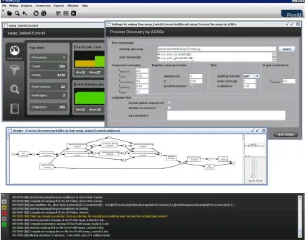
AGNEs has been implemented in Prolog. In particular, the frequent temporal constraint induction, the artificial negative event generation, the language bias constraints, and the pruning and graph construction algorithms all have been written in Prolog. As mentioned before, AGNEs makes use of TILDE, an existing multi-relational classifier (Blockeel and De Raedt, 1998), available in the ACE-ilProlog data mining system (Blockeel et al., 2002). To be able to benefit from the facilities of the ProM framework, a plugin was written that makes AGNEs accessible in ProM.1Figure 3 depicts a screen shot of AGNEs in ProM.

In this section the results of an experimental evaluation of AGNEs are presented. First we will discuss the properties of the event logs and the parameter settings that have been used. Then, in Section 6.1, we analyse the expressiveness of AGNEs and benchmark the ability of AGNEs to generalize from incomplete event logs. In Section 6.2, we analyze the results of a number of noise experiments with different types and levels of noise that have been carried out to test how the learning algorithm behaves in the presence of noise.

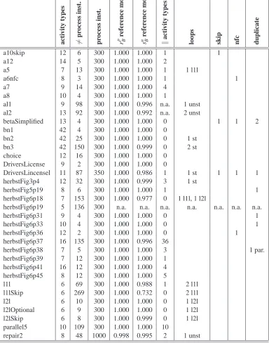
In order to evaluate and compare the performance of AGNEs, a benchmark experiment with 34 event logs has been set up. These event logs have previously been used by Alves de Medeiros (2006) and Alves de Medeiros et al. (2007) to evaluate the genetic miner algorithm. Table 1 describes the properties of the underlying artificial process models of the event logs. The number of different process instance sequences (column “6=process inst.”) gives an indication of the amount of different behavior that is present in the event log. This number is to be compared with the total number of process instances in the event logs. In general, the presence of loops and parallelism exponentially increases the amount of different behavior that can be produced by a process. Therefore, the number of activity types that are pairwise parallel and the number and type of loops have been reported in Table 1. In correspondence with the naming conventions used by Alves de Medeiros, nfc stands for

non-free-choice, l1l and l2l stands for the presence of a length-one and length-two loop respectively, and st and unst stands for structured and unstructured loops. Furthermore, the presences of special structures such as skip activities and (parallel or serial) duplicate activities have been indicated. For most of the event logs in the experiment, a reference model was available that can be assumed to represent the behavior in the event log. Columns “r_Bp reference model” and “sn_B reference model” indicate the behavioral recall and specificity of the reference models with respect to the original event logs.

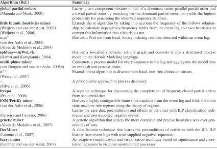
In the experiments, the performance of AGNEs is compared to the performance of four state-of-the-art process discovery algorithms: α+ (van der Aalst et al., 2004; Alves de Medeiros et al., 2004),α++(Wen et al., 2007), genetic miner (Alves de Medeiros et al., 2007) and heuristics miner (Weijters et al., 2006). Being the first large-scale, comparative benchmark study in the literature of process discovery, we have chosen to include algorithms that already have appeared as journal publications (α+,α++, and genetic miner) or that are much referenced in the literature (heuristics miner).

During all experiments, the algorithms were run with the same, standard parameter settings of their ProM 4.2 implementation, as reported in Table 2. These parameter settings coincide with the ones used to run similar experiments by the authors of the algorithms. To enable a comparison on the same terms, AGNEs was not provided with prior knowledge regarding parallelism or locality of activity types. In particular, the thresholds used to induce frequent temporal patterns have been given the following values (tabsence= 0.9, tchain = 0.08, tsucc= 0.8, tordering= 0.08, ttriple = 0.10). In practice, a good threshold depends on the amount of low-frequent behavior (noise) one is willing to accept within the discovered process model. The negative event injection probabilityπinfluences the proportion of artificially generated negative events in an event log. A strong imbalance of this proportion may bias a classification learner towards a majority class prediction, without deriving any useful preconditions for a particular activity type. As a rule of thumb, it is a good idea to set this parameter value as low as possible, without the learner making a majority class prediction. In the experimentsπhas been given a default value of 0.08. Ex-post, AGNEs warns the user when too low a value forπhas led to a majority-class prediction. TILDE’s C4.5 gain metric was used as a heuristic for selecting the best branching criterion. In addition, TILDE’s C4.5 post pruning method was used with a standard confidence level of 0.25. Furthermore, TILDE is forced to stop node splitting when the number of process instances in a tree node drops below 5. The same parameter settings have been used on all 34 data sets. Empirical validation has shown the parameter settings to work well across all data sets.

The AGNEs technique, has run times in between 20 seconds and 2 hours for the data sets in the experiments on a Pentium 4, 2.4 Ghz machine with 1GB internal memory. These processing times are well in excess of the processing times ofα+,α++and heuristics miner. In comparison to the run times of the genetic miner algorithm, processing times are considerably shorter. Most of the time is required by TILDE to learn the preconditions for each activity type. The generation of negative events also can take up some time. As process discovery generally is not a real-time data mining application, less attention has been given to computation times.

6.1 Zero-noise, Cross Validation Experiment

ac

ti

vit

y

type

s

6

=

pr

oc

es

s

in

st

.

pr

oc

es

s

in

st

.

r

p B

re

fe

re

nc

e

m

ode

l

s

n B

re

fe

re

nc

e

m

ode

l

k

ac

ti

vit

y

type

s

loop

s

sk

ip

nf

c

du

plic

at

e

a10skip 12 6 300 1.000 1.000 1 1

a12 14 5 300 1.000 1.000 2

a5 7 13 300 1.000 1.000 1 1 l1l

a6nfc 8 3 300 1.000 1.000 1 1

a7 9 14 300 1.000 1.000 4

a8 10 4 300 1.000 1.000 1

al1 9 98 300 1.000 0.996 n.a. 1 unst

al2 13 92 300 1.000 0.992 n.a. 2 unst

betaSimplified 13 4 300 1.000 1.000 0 1 1 2

bn1 42 4 300 1.000 1.000 0

bn2 42 25 300 1.000 1.000 0 1 st

bn3 42 150 300 1.000 0.999 0 2 st

choice 12 16 300 1.000 1.000 0

DriversLicense 9 2 300 1.000 1.000 0

DriversLincensel 11 87 350 1.000 0.986 1 1 st 1 1 1

herbstFig3p4 12 32 300 1.000 0.999 3 1 st

herbstFig5p19 8 6 300 1.000 1.000 1 1

herbstFig6p18 7 153 300 1.000 0.977 0 1 l1l, 1 l2l

herbstFig6p19 5 136 300 n.a. n.a. n.a. n.a. n.a. n.a. n.a.

herbstFig6p31 9 4 300 1.000 1.000 0 1

herbstFig6p33 10 4 300 1.000 1.000 0 1

herbstFig6p36 12 2 300 1.000 1.000 0 1

herbstFig6p37 16 135 300 1.000 0.996 36

herbstFig6p38 7 5 300 1.000 1.000 3 1 par.

herbstFig6p39 7 12 300 1.000 1.000 1 herbstFig6p41 16 12 300 1.000 1.000 4 herbstFig6p45 8 12 300 1.000 1.000 5

l1l 6 69 300 1.000 0.988 1 2 l1l

l1lSkip 6 269 300 1.000 0.732 0 2 l1l

l2l 6 10 300 1.000 1.000 0 1 l2l

l2lOptional 6 9 300 1.000 1.000 0 1 l2l

l2lSkip 6 8 300 1.000 0.999 0 1 l2l

parallel5 10 109 300 1.000 1.000 10

repair2 8 48 1000 0.998 0.995 2 1 unst

Table 1: Event log properties

Algorithm (Ref.) Parameter settings

α+

(Alves de Medeiros et al., 2004)

derive succession from partial order information = true

enforce causal dependencies within events of the same activity = false enforce parallelism by overlapping events = false

α++

(Wen et al., 2007)

(no settings)

heuristics miner Weijters et al. (2006)

relative to best threshold = 0.05 positive observations = 10 dependency threshold = 0.9 length-one-loops threshold = 0.9 length-two-loops threshold = 0.9 long-distance threshold = 0.9 dependency divisor = 1 and threshold = 0.1

use all-activities-connected heuristic = true use long-distance dependency heuristic = false

genetic miner

(Alves de Medeiros et al., 2007)

population size = 100

max number generations = 1000

initial population type = possible duplicates power value = 1

elitism rate = 0.2

selection type = tournament 5

extra behavior punishment withκ= 0.025

enhanced crossover type with crossover probability = 0.8 enhanced mutation type with mutation probability = 0.2

AGNEs

prior knowledge none

temporal constraints tabsence= 0.9, tchain= 0.08, tsucc= 0.8,

tordering= 0.08, ttriple= 0.1 negative event generation injection probabilityπ= 0.08

calculate parallel variants = true include global sequences = true language bias: include occurrence count = false

data conditions = none

TILDE splitting heuristic: gain

minimal cases in tree nodes = 5

C4.5 pruning with confidence level = 0.25 graph construction tconnect= 0.4

Table 2: Parameter settings

written in SWI-Prolog that groups similar sequences, randomly partitions the grouped event log in n=10 uniform subgroups, and produces n pairs of training and test event logs. Training event logs are used for the purpose of process discovery. Test event logs are used for evaluation, this is for calculating the specificity and recall metrics. For the purpose of this experiment, no noise was added to the event logs.

an injection probabilityπequal to 1, an infinite window size, and by considering parallel variants. Evidently, the thus generated negative events were not retained in the training set. For training purposes, negative events have been calculated based on the information in the training set only. For the same reasons, the behavioral appropriateness metric a′_B has also been calculated based on the whole of training and test set data.

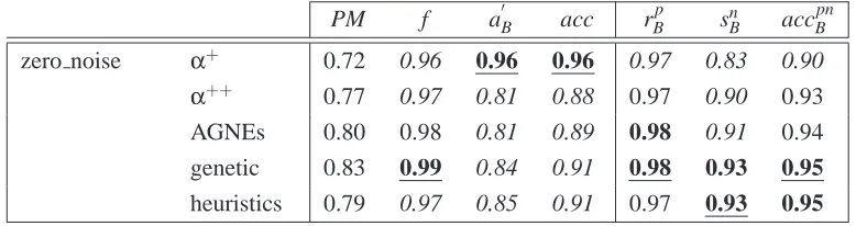
In the experiment, only 19 out of the 34 event logs were retained, as the other event logs have less than 10 different sequences. Table 3 shows the aggregated, average results of the 10-fold cross validation experiment over 190 event logs. The best average performance over the 34 event logs is underlined and denoted in bold face for each metric. We then use a paired t-test to test the significance of the performance differences (Van Gestel et al., 2004). Performances that are not significantly different at the 5% level from the top-ranking performance with respect to a one-tailed paired t-test are tabulated in bold face. Statistically significant underperformances at the 1% level are emphasized in italics. Performances significantly different at the 5% level but not at the 1% level are reported in normal font. For the PM measure, no paired t-tests could be performed, because the metric could not be calculated on some of the process models discovered byα+ and α++_{. The latter is the case when the discovered process models have disconnected elements.}

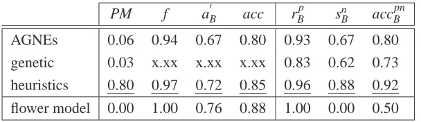
From the results for the parsing measure PM, the fitness measure f , and behavioral recall mea-sures r_Bp, it can be concluded that genetic miner scores slightly better on the recall requirement. Moreover, the behavioral specificity metric sn_Bshows genetic miner and heuristics miner to produce slightly more specific models.

PM f a′_B acc r_Bp sn_B acc_Bpn

zero noise α+ 0.72 0.96 0.96 0.96 0.97 0.83 0.90

α++ _{0.77 0.97 0.81 0.88 0.97 0.90 0.93}

AGNEs 0.80 0.98 0.81 0.89 0.98 0.91 0.94

genetic 0.83 0.99 0.84 0.91 0.98 0.93 0.95

heuristics 0.79 0.97 0.85 0.91 0.97 0.93 0.95

Table 3: 10-fold cross validation experiment - aggregated results

A A

A Artif icialEndT ask

Artif icialStartT ask

B C D

E

F G H

(a) AGNEs result

Artif icialStartT ask

A

D F

Artif icialEndT ask

E H

B G

C

(b) heuristics miner result

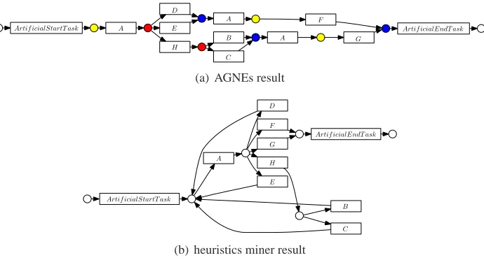
Figure 2: herbstFig6p33: AGNEs detects the duplicate activity A

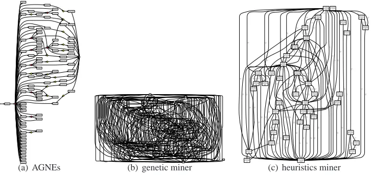
The metrics r_Bp and sn_B do not indicate a large or significant difference for the performance of α++_{, AGNEs, genetic miner, and heuristics miner. Only by looking at the individual process} mod-els, the expressiveness of AGNEs with respect to the detection of non-local, non-free choice con-structs or the discovery of duplicate tasks becomes apparent. Example 3, discussed in Section 4.3, shows how AGNEs is capable of detecting non-local, non-free choice constructs, even within the loop of the DriversLicensel reference problem. AGNEs is also particularly suited for the detection of duplicate activities. In the herbstFig6p33 event log, the activity A occurs in three different con-texts and AGNEs draws three different, identically labeled transitions correspondingly. Figure 2 compares the results of heuristics miner and AGNEs on this event log.

The goal of process discovery is to give an idea of how the processes recorded in the event log actually have taken place. This goal makes process discovery an inherently descriptive learning task. To evaluate the accuracy of the discovered process model, it is therefore justified to compare the learned process models on the same sequence the process models are learned from. In the process discovery literature, this training-log-based evaluation has been the dominant evaluation paradigm (Alves de Medeiros et al., 2007; Weijters et al., 2006). Consequently, the remaining experiments of this paper use training-log-based evaluation.

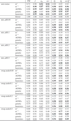
6.2 Training-log-based Noise Experiment