Learning Image Components for Object Recognition
Michael W. Spratling [email protected]
Division of Engineering
King’s College London, UK, and
Centre for Brain and Cognitive Development Birkbeck College, London, UK
Editor: Peter Dayan
Abstract
In order to perform object recognition it is necessary to learn representations of the underlying components of images. Such components correspond to objects, object-parts, or features. Non-negative matrix factorisation is a generative model that has been specifically proposed for finding such meaningful representations of image data, through the use of non-negativity constraints on the factors. This article reports on an empirical investigation of the performance of non-negative matrix factorisation algorithms. It is found that such algorithms need to impose additional con-straints on the sparseness of the factors in order to successfully deal with occlusion. However, these constraints can themselves result in these algorithms failing to identify image components under certain conditions. In contrast, a recognition model (a competitive learning neural network algorithm) reliably and accurately learns representations of elementary image features without such constraints.
Keywords: non-negative matrix factorisation, competitive learning, dendritic inhibition, object recognition
1. Introduction
have previously been applied to this test problem, and neural networks are a standard technique for learning object representations, the performance of NMF is compared to that of an unsupervised neural network learning algorithm applied to the same set of tasks.
2. Method
This section describes the NMF algorithms, and the neural network algorithms, which are explored in this paper. The performance of these algorithms is compared in the Results section.
2.1 Non-Negative Matrix Factorisation
Given an m by p matrix X= [~x1, . . . ,~xp], each column of which contains the pixel values of an image (i.e., X is a set of training images), the aim is to find the factors A and Y such that
X≈AY,
where A is an m by n matrix the columns of which contain basis vectors, or components, into which the images can be decomposed, and Y= [~y1, . . . ,~yp]is an n by p matrix containing the activations of each component (i.e., the strength of each basis vector in the corresponding training image). A training image (~xk) can therefore be reconstructed as a linear combination of the image components contained in A, such that~xk≈A~yk.
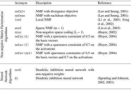
A number of different learning algorithms can be defined depending on the constraints that are placed on the factors A and Y. For example, vector quantization (VQ) restricts each column of Y to have only one non-zero element, principal components analysis (PCA) constrains the columns of A to be orthonormal and the rows of Y to be mutually orthogonal, and independent components analysis (ICA) constrains the rows of Y to be statistically independent. Non-negative matrix factori-sation is a method that seeks to find factors (of a non-negative matrix X) under the constraint that both A and Y contain only elements with non-negative values. It has been proposed that this method is particularly suitable for finding the components of images, since from the physical properties of image formation it is known that image components are non-negative and that these components are combined additively (i.e., are not subtracted) in order to generate images. Several different algo-rithms have been proposed for finding the factors A and Y under non-negativity constraints. Those tested here are listed in Table 1.
Algorithms nmfdiv and nmfmse impose non-negativity constraints solely, and differ only in the objective function that is minimised in order to find the factors. All the other algorithms ex-tend non-negative matrix factorisation by imposing additional constraints on the factors. Algorithm
Acronym Description Reference N o n -n eg ati v e M atr ix F ac to ris atio n A lg o rith ms
nmfdiv NMF with divergence objective (Lee and Seung, 2001)
nmfmse NMF with euclidean objective (Lee and Seung, 2001)
lnmf Local NMF (Li et al., 2001; Feng
et al., 2002)
snmf Sparse NMF (α=1) (Liu et al., 2003)
nnsc Non-negative sparse coding (λ=1) (Hoyer, 2002)
nmfsc (A) NMF with a sparseness constraint of 0.5 on the basis vectors
(Hoyer, 2004)
nmfsc (Y) NMF with a sparseness constraint of 0.7 on the activations
(Hoyer, 2004)
nmfsc (A&Y) NMF with sparseness constraints of 0.5 on the basis vectors and 0.7 on the activations
(Hoyer, 2004) N eu ra l N etw o rk A lg o rith
ms nndi Dendritic inhibition neural network with
non-negative weights
di Dendritic inhibition neural network (Spratling and Johnson,
2002, 2003)
Table 1: The algorithms tested in this article. These include a number of different algorithms for finding matrix factorisations under non-negativity constraints and a neural network algo-rithm for performing competitive learning through dendritic inhibition.
of Y had a sparseness of 0.7 (where sparseness is in the range[0,1], as for the constraint on A). For
nmfsc (A&Y)these same constraints were imposed on both the sparseness of basis vectors and the activations. For thenmfscalgorithm, fixed values for the parameters controlling sparseness were used in order to provide a fairer comparison with the other algorithms all of which used constant parameter settings. Furthermore, since all the test cases studied are very similar, it is reasonable to expect an algorithm to work across them all without having to be tuned specifically to each individ-ual task. The particular parameter values used were selected so as to provide the best overall results across all the tasks. The effect of changing the sparseness parameters is described in the discussion section.
2.2 Dendritic Inhibition Neural Network
Weights
Feedback
1k 2k
1k 2k 3k
11
X
Y
Y
X
X
A
(a)
Feedforward Weights
1k 2k
1k 2k 3k
11
X
Y
Y
X
X
W
(b)
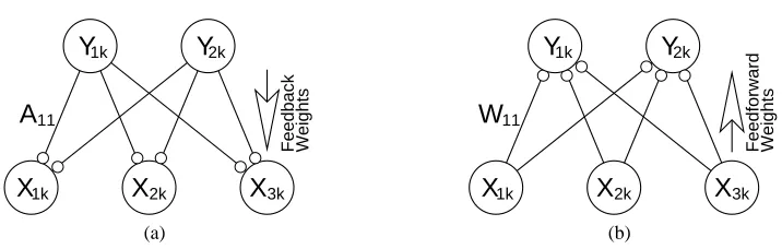
Figure 1: (a) A generative neural network model: feedback connections enable neural activations (~yk) to reconstruct an input pattern (~xk). (b) A recognition neural network model: feed-forward connections cause neural activations (~yk) to be generated in response to an input pattern (~xk). Nodes are shown as large circles and excitatory synapses as small open circles.
such that
Y=f(W,X),
where W is an n by m matrix of synaptic weight values, X= [~x1, . . . ,~xp]is an m by p matrix of training images, and Y= [~y1, . . . ,~yp]is an n by p matrix containing the activation of each node in response to the corresponding image. Typically, the rows of W form templates that match image features, so that individual nodes become active in repose to the presence of specific components of the image. Nodes thus act as ‘feature detectors’ (Barlow, 1990, 1995).
Many different functions are possible for calculating neural activations and many different learn-ing rules can be defined for findlearn-ing the values of W. For example, algorithms have been proposed for performing vector quantization (Kohonen, 1997; Ahalt et al., 1990), principal components analysis (Oja, 1992; Fyfe, 1997b; F¨oldi´ak, 1989), and independent components analysis (Jutten and Herault, 1991; Charles and Fyfe, 1997; Fyfe, 1997a). Many of these algorithms impose non-negativity con-straints on the elements of Y and W for reasons of biological plausibility, since neural firing rates are positive and since synapses can not change between being excitatory and being inhibitory. In general, such algorithms employ different forms of competitive learning, in which nodes compete to be active in response to each input pattern. Such competition can be implemented using a number of different forms of lateral inhibition. In this paper, a competitive learning algorithm in which nodes can inhibit the inputs to other nodes is used. This form of inhibition has been termed dendritic inhibition or pre-integration lateral inhibition. The full dendritic inhibition model (Spratling and Johnson, 2002, 2003) allows negative synaptic weight values. However, in order to make a fairer comparison with NMF, a version of the dendritic inhibition algorithm in which all synaptic weights are restricted to be non-negative (by clipping the weights at zero) is also used in the experiments described here. The full model will be referred to by the acronymdiwhile the non-negative version will be referred to asnndi(see Table 1).
In a neural network model, an input image (~xk) generates activity (~yk) in the nodes of a neural network such that~yk=f(W,~xk). In the dendritic inhibition model, the activation of each individual node is calculated as:
where~x′k j is an inhibited version of the input activations (~xk) that can differ for each node. The values of~x′k jare calculated as:
xik j′ =xik
1−α
n max
r=1
(r6=j)
(
wri
maxmq=1wrq
yrk
maxnq=1yqk ) + ,
whereαis a scale factor controlling the strength of lateral inhibition, and(v)+ is the positive half-rectified value of v. The steady-state values of yjkwere found by iteratively applying the above two equations, increasing the value of α from 0 to 6 in steps of 0.25, while keeping the input image fixed.
The above activation function implements a form of lateral inhibition in which each neuron can inhibit the inputs to other neurons. The strength with which a node inhibits an input to another node is proportional to the strength of the afferent weight the inhibiting node receives from that particular input. Hence, if a node is strongly activated by the overall stimulus and it has a strong synaptic weight to a certain feature of that stimulus, then it will inhibit other nodes from responding to that feature. On the other hand, if an active node receives a weak weight from a feature then it will only weakly inhibit other nodes from responding to that feature. In this manner, each node can selectively ‘block’ its preferred inputs from activating other nodes, but does not inhibit other nodes from responding to distinct stimuli.
All weight values were initialised to random values chosen from a Gaussian distribution with a mean of m1 and a standard deviation of 0.001mn. This small degree of noise on the initial weight values was sufficient to cause bifurcation of the activity values, and thus to cause differentiation of the receptive fields of different nodes through activity-dependent learning. Previous results with this algorithm have been produced using noise (with a similarly small magnitude) applied to the node activation values. Using noise applied to the node activations, rather than the weights, produces similar results to those reported in this article. However, noise was only applied to the initial weight values, and not to the node activations, here to provide a fairer comparison to the deterministic NMF algorithms. Note that a node which still has its initial weight values (i.e., a node which has not had its weights modified by learning) is described as ‘uncommitted’.
Synaptic weights were adjusted using the following learning rule (applied to weights with values greater than or equal to zero):
∆wji=
(xik−x¯k) ∑m
p=1xpk
yjk−y¯k
+
. (1)
Here ¯xkis the mean value of the pixels in the training image (i.e., ¯xk=m1∑mi=1xik), and ¯ykis the mean of the output activations (i.e., ¯yk= 1n∑nj=1yjk). Following learning, synaptic weights were clipped at zero such that wji= (wji)+and were normalised such that∑im=1(wji)+≤1.
post-synaptic term of the rule so that no weight changes occur when the node is less active than average. If learning was not restricted in this way, whenever a pattern was presented all nodes which represented patterns with overlapping features would reduce their weights to these features.
For the algorithm di, but not for algorithm nndi, the following learning rule was applied to weights with values less than or equal to zero:
∆wji=
x′ik j−0.5xik
−
∑n p=1ypk
yjk−y¯k
. (2)
Here (v)− is the negative half-rectified value of v. Negative weights were clipped at zero such that wji= (wji)− and were normalised such that∑im=1(wji)− ≥ −1. Note that for programming convenience a single synapse is allowed to take either excitatory or inhibitory weight values. In a more biologically plausible implementation two separate sets of afferent connections could be used: the excitatory ones being trained using equation 1 and the inhibitory ones being trained using a rule similar to equation 2.
The negative weight learning rule has a different form from the positive weight learning rule as it serves a different purpose. The negative weights are used to ensure that each image component is represented by a distinct node rather than by the partial activation of multiple nodes each of which represents an overlapping image component. A full explanation of this learning rule is provided together with a concrete example of its function in section 3.3.
3. Results
In each of the experiments reported below, all the algorithms listed in Table 1 were applied to learning the components in a set of p training images. The average number of components that were correctly identified over the course of 25 trials was recorded. A new set of p randomly generated images were created for each trial. In each trial the NMF algorithms were trained until the total sum of the absolute difference in the objective function, between successive epochs, had not changed by more than 0.1% of its average value in 100 epochs, or until 2000 epochs had been completed. One epoch is when the method has been trained on all p training patterns. Hence, an epoch equals one update to the factors in an NMF algorithm, and p iterations of the neural network algorithm during which each individual image in the training set is presented once as input to the network. The neural network algorithms were trained for 10000 iterations. Hence, the NMF algorithms were each trained for at least 100 epochs, while the neural network algorithms were trained for at most 100 epochs (since the value of p was 100 or greater).
3.1 Standard Bars Problem
Figure 2: Typical training patterns for the standard bars problem. Horizontal and vertical bars in 8x8 pixel images are independently selected to be present with a probability of 18. Dark pixels indicate active inputs.
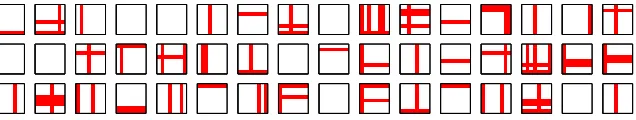
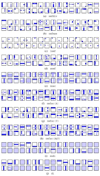
In the first experiment the algorithms were trained on the standard bars problem. Twenty-five trials were performed with p=100, and, with p=400. The number of components that each algorithm could learn (n) was set to 32. Typical examples of the (generative) weights learnt by each NMF algorithm (i.e., the columns of A reshaped as 8 by 8 pixel images) and of the (recognition) weights learnt by the neural network algorithms (i.e., the rows of W reshaped as 8 by 8 pixel images) are shown in Figure 3. It can be seen that the NMF algorithms tend to learn a redundant representation, since the same bar can be represented multiple times. In contrast, the neural network algorithms learnt a much more compact code, with each bar being represented by a single node. It can also be seen that many of the NMF algorithms learnt representations of bars in which pixels were missing. Hence, these algorithms learnt random pieces of image components rather than the image components themselves. In contrast, the neural network algorithms (and algorithms nnsc,
nmfsc (A), andnmfsc (A&Y)) learnt to represent complete image components.
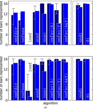
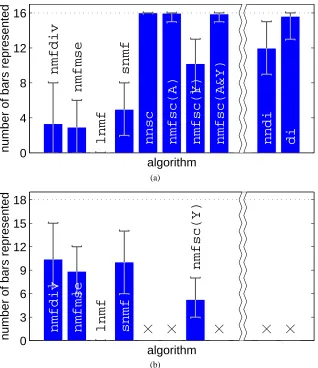
To quantify the results, the following procedure was used to determine the number of bars represented by each algorithm in each trial. For each node, the sum of the weights corresponding to each row and column of the input image was calculated. A node was considered to represent a particular bar if the total weight corresponding to that bar was twice that of the sum of the weights for any other row or column and if the minimum weight in the row or column corresponding to that bar was greater than the mean of all the (positive) weights for that node. The number of unique bars represented by at least one basis vector, or one node of the network, was calculated, and this value was averaged over the 25 trials. The mean number of bars (i.e., image components) represented by each algorithm is shown in Figure 4a. Good performance requires both accuracy (finding all the image components) and reliability (doing so across all trials). Hence, the average number of bars represented needs to be close to 16 for an algorithm to be considered to have performed well. It can be seen that when p=100, most of the NMF algorithms performed poorly on this task. However, algorithmsnmfsc (A)andnmfsc (A&Y)produced good results, representing an average of 15.7 and 16 components respectively. This compares favourably to the neural network algorithms, withnndi
representing 14.6 and di representing 15.9 of the 16 bars. When the number of images in the training set was increased to 400 this improved the performance of certain NMF algorithms, but lead to worse performance in others. For p=400, every image component in every trial was found by algorithmsnnsc,nmfsc (A),nmfsc (A&Y)anddi.
(a) nmfdiv
(b) nmfmse
(c) lnmf
(d) snmf
(e) nnsc
(f) nmfsc (A)
(g) nmfsc (Y)
(h) nmfsc (A&Y)
(i) nndi
(j) di
0
4
8
12
16
number of bars represented
nmfdiv
nmfmse
lnmf
snmf
nnsc
nmfsc(A)
nmfsc(Y)
nmfsc(A&Y)
nndi
di
algorithm
(a)0
4
8
12
16
number of bars represented
nmfdiv
nmfmse
lnmf
snmf
nnsc
nmfsc(A)
nmfsc(Y)
nmfsc(A&Y)
nndi
di
algorithm
(b)Figure 4: Performance of each algorithm when trained on the standard bars problem. For (a) 32, and (b) 16 basis vectors or nodes. Each bar shows the mean number of components correctly identified by each algorithm when tested over 25 trials. Results for different training set sizes are shown: the lighter, foreground, bars show results for p=100, and the darker, background, bars show results for p=400. Error bars show best and worst performance, across the 25 trials, when p=400.
learn image components with an excess of nodes. Across both these experiment thediversion of the neural network algorithm performs as well as or better than any of the NMF algorithms.
3.2 Bars Problems Without Occlusion
To determine the effect of occlusion on the performance of each algorithm further experiments were performed using versions of the bars problem in which no occlusion occurs. Firstly, a linear version of the standard bars problem was used. Similar tasks have been used by Plumbley (2001) and Hoyer (2002). In this task, pixel values are combined additively at points of overlap between horizontal and vertical bars. As with the standard bars problem, training data consisted of 8 by 8 pixel images in which each of the 16 possible (one-pixel wide) horizontal and vertical bars could be present with a probability of 18. All the algorithms were trained with p=100 and with p=400 using 32 nodes or basis vectors. The number of unique bars represented by at least one basis vector, or one node of the network, was calculated, and this value was averaged over 25 trials. The mean number of bars represented by each algorithm is shown in Figure 5a.
Another version of the bars problem in which occlusion is avoided is one in which horizontal and vertical bars do not co-occur. Similar tasks have been used by Hinton et al. (1995); Dayan and Zemel (1995); Frey et al. (1997); Hinton and Ghahramani (1997) and Meila and Jordan (2000). In this task, an orientation (either horizontal or vertical) was chosen with equal probability for each training image. The eight (one-pixel wide) bars of that orientation were then independently selected to be present with a probability of 18. All the algorithms were trained with p=100 and with p=400 using 32 nodes or basis vectors. The number of unique bars represented by at least one basis vector, or one node of the network, was calculated, and this value was averaged over 25 trials. The mean number of bars represented by each algorithm is shown in Figure 5b.
For both experiments using training images in which occlusion does not occur, the performance of most of the NMF algorithms is improved considerably in comparison to the standard bars prob-lem. The neural network algorithms also reliably learn the image components as with the standard bars problem.
3.3 Bars Problem with More Occlusion
To further explore the effects of occlusion on the learning of image components a version of the bars problem with double-width bars was used. Training data consisted of 9 by 9 pixel images in which each of the 16 possible (two-pixel wide) horizontal and vertical bars could be present with a probability 18. The image size was increased by one pixel to keep the number of image components equal to 16 (as in the previous experiments). In this task, as in the standard bars problem, perpendicular bars overlap; however, the proportion of overlap is increased. Furthermore, neighbouring parallel bars also overlap (by 50%). Typical examples of training images are shown in Figure 6.
0
4
8
12
16
number of bars represented
nmfdiv
nmfmse
lnmf
snmf
nnsc
nmfsc(A)
nmfsc(Y)
nmfsc(A&Y)
nndi
di
algorithm
(a)0
4
8
12
16
number of bars represented
nmfdiv
nmfmse
lnmf
snmf
nnsc
nmfsc(A)
nmfsc(Y)
nmfsc(A&Y)
nndi
di
algorithm
(b)Figure 5: Performance of each algorithm when trained on (a) the linear bars problem, and (b) the one-orientation bars problem, with 32 basis vectors or nodes. Each bar shows the mean number of components correctly identified by each algorithm when tested over 25 trials. Results for different training set sizes are shown: the lighter, foreground, bars show results for p=100, and the darker, background, bars show results for p=400. Error bars show best and worst performance, across the 25 trials, when p=400.
Figure 6: Typical training patterns for the double-width bars problem. Two pixel wide horizontal and vertical bars in a 9x9 pixel image are independently selected to be present with a probability of18. Dark pixels indicate active inputs.
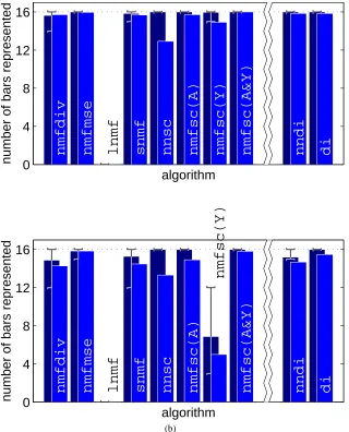
for that node. The number of unique bars represented by at least one basis vector, or one node of the network, was calculated. The mean number of two-pixel-wide bars, over the 25 trials, represented by each algorithm is shown in Figure 8a. This set of training images could be validly, but less ef-ficiently, represented by 18 one-pixel-wide bars. Hence, the mean number of one-pixel-wide bars, represented by each algorithm was also calculated and this data is shown in Figure 8b. The number of one-pixel-wide bars represented was calculated using the same procedure used to analyse the previous results (as stated in section 3.1).
It can be seen that the majority of the NMF algorithms perform very poorly on this task. Most fail to reliably represent either double- or single-width bars. However, algorithmsnnsc,nmfsc (A)
(a) nmfdiv
(b) nmfmse
(c) lnmf
(d) snmf
(e) nnsc
(f) nmfsc (A)
(g) nmfsc (Y)
(h) nmfsc (A&Y)
(i) nndi
(j) di
0
4
8
12
16
number of bars represented
nmfdiv
nmfmse
lnmf
snmf
nnsc
nmfsc(A)
nmfsc(Y)
nmfsc(A&Y)
nndi
di
algorithm
(a)0
3
6
9
12
15
18
number of bars represented
nmfdiv
nmfmse
lnmf
snmf
nmfsc(Y)
algorithm
(b)Figure 8: Performance of each algorithm when trained on the double-width bars problem, with 32 basis vectors or nodes, and p=400. Each bar shows the mean number of components correctly identified by each algorithm when tested over 25 trials. (a) Number of double-width bars learnt. (b) Number of single-double-width bars learnt. Error bars show best and worst performance across the 25 trials. Note that algorithms that successfully learnt double-width bars—see (a)—do not appear in (b), but space is left for these algorithms in order to aid comparison between figures.
co-activation of independent input patterns then the weights will return toward zero on subsequent presentations of these patterns in isolation.
3.4 Bars Problem with Unequal Components
1k
1k 2k 3k
X
Y
X
X
Y
2kY
3kX
4kbar 1
bar 2
bar 3
Figure 9: An illustration of a the role of negative weights in the dendritic inhibition algorithm. Nodes are shown as large circles, excitatory synapses as small open circles and inhibitory synapses as small filled circles. Nodes Y1k and Y3k are selective for the double-width
bars 1 and 3 respectively. The occurrence in an image of the double-width bar ‘bar 2’ would be indicated by both nodes Y1k and Y3kbeing active at half-strength. However, if
bar 2 occurs sufficiently frequently, the negative afferent weights indicated will develop which will suppress this response and enable the uncommitted node (Y2k) to compete to
respond to this pattern. Note that each bar would activate two columns each containing eight input nodes, but only one input node per column is shown for clarity.
same probability. This is unlikely to be the case in world object recognition tasks. In the real-world, different image features can be radically different in size and can be encountered with very different frequency. For example, important features in face recognition include both the eyes and the hair (Sinha and Poggio, 1996; Davies et al., 1979) which can vary significantly in relative size. Furthermore, we effortlessly learn to recognise both immediate family members (who may be seen many times a day) and distant relatives (who may be seen only a few times a year).
To provide a more realistic test, a new variation on the bars problem was used. In this version, training data consisted of 16 by 16 pixel images. Image components consisted of seven one-pixel wide bars and one nine-pixel wide bar in both the horizontal and vertical directions. Hence, as in previous experiments, there were eight image components at each orientation and 16 in total. Parallel bars did not overlap, however, the proportion of overlap between the nine-pixel wide bars and all other perpendicular bars was large, while the proportion of overlap between perpendicular one-pixel wide bars was less than in the standard bars problem. Each horizontal bar was selected to be present in an image with a probability of 18 while vertical bars occurred with a probability of321. Hence, in this test case half the underlying image components occurred at a different frequency to the other half and two of the components were a different size to the other 14.
0
4
8
12
16
number of bars represented
nmfdiv
nmfmse
lnmf
snmf
nnsc
nmfsc(A)
nmfsc(Y)
nmfsc(A&Y)
nndi
di
algorithm
Figure 10: Performance of each algorithm when trained on the unequal bars problem, with 32 basis vectors or nodes, and p=400. Each bar shows the mean number of components cor-rectly identified by each algorithm when tested over 25 trials. Error bars show best and worst performance across the 25 trials.
the two large components appears to be a particular problem for all these algorithms, but the cause for this may differ between algorithms. For most NMF algorithms, the underlying linear model fails when occlusion is significant, as is the case for the two nine-pixel wide patterns. However, for the NMF algorithms that find non-negative factors with an additional constraint on the sparseness of the basis vectors (i.e.,nmfsc (A)andnmfsc (A&Y)) an alternative cause may be the imposition of a constraint that requires learnt image components to be a similar size, which is not the case for the components used in this task. The neural network algorithm with positive weights (nndi) produced results that are only marginally better than the NMF algorithms. This algorithm also fails to reliably learn the two large components due to the large overlap between them. In contrast, the dendritic inhibition neural network algorithm with negative weights (di), succeeded in identifying all the bars in most trials. As for the previous experiment with double-width bars, this result illus-trates the need to allow negative weight values in this algorithm in order to robustly learn image components. Algorithmdilearnt every image component in 18 of the 25 trials. In contrast, only one NMF algorithm (nnsc) managed to find all the image components, but it only did so in a single trial.
3.5 Face Images
Previously, NMF algorithms have been tested using a training set that consists of images of faces (Lee and Seung, 1999; Hoyer, 2004; Li et al., 2001; Feng et al., 2002). When these training images are taken from the CBCL face database,1 algorithmnmfdiv learns basis vectors that correspond to localised image parts (Lee and Seung, 1999; Hoyer, 2004; Feng et al., 2002). However, when
1. CBCL Face Database #1, MIT Center For Biological and Computation Learning,
(a) nndi
(b) di
Figure 11: (a) and (b) Typical recognition weights learnt by 32 nodes when both versions of the dendritic inhibition algorithm were trained on the CBCL face database. Light pixels indicate strong weights.
applied to the ORL face database,2 algorithmnmfmselearns global, rather than local, image fea-tures (Li et al., 2001; Hoyer, 2004; Feng et al., 2002). In contrast, algorithmlnmflearns localised representations of the ORL face database (Feng et al., 2002; Li et al., 2001). Algorithmnmfsccan find either local or global representations of either set of face images with appropriate values for the constraints on the sparseness of the basis vectors and activations. Specifically, nmfsc learns localised image parts when constrained to produce highly sparse basis images, but learns global image features when constrained to produce basis images with low sparseness or if constrained to produce highly sparse activations (Hoyer, 2004). Hence, NMF algorithms can, in certain circum-stances, learn localised image components, some of which appear to roughly correspond to parts of the face, but others of which are arbitrary, but localised, blobs. Essentially the NMF algorithms se-lect a subset of the pixels which are simultaneously active across multiple images to be represented by a single basis vector. The same behaviour is observed in the bars problems, reported above, where a basis vector often corresponds to a random subset of pixels along a row or column of the image rather than representing an entire bar. Such arbitrary image components are not meaningful representations of the image data.
In contrast when the dendritic inhibition neural network is trained on face images, it learns global representations. Figure 11a and Figure 11b show the results of training nndi anddi, for 10000 iterations, on the 2429 images in the CBCL face database. Parameters were identical to those used for the bars problems, except the weights were initialised to random values chosen from a Gaussian distribution with a larger standard deviation (0.005mn) as this was found necessary to cause bifurcation of activity values. In both cases, each node has learnt to represent an average (or prototype) of a different subset of face images. When presented with highly overlapping training images the neural network algorithm will learn a prototype consisting of the common features be-tween the different images (Spratling and Johnson, 2006). When presented with objects that have less overlap, the network will learn to represent the individual exemplars (Spratling and Johnson, 2006). These two forms of representation are believed to support perceptual categorisation and object recognition (Palmeri and Gauthier, 2004).
2. The ORL Database of Faces, AT&T Laboratories Cambridge,
4. Discussion
The NMF algorithmlnmfimposes the constraint that the basis vectors be orthogonal. This means that image components may not overlap and, hence, results in this algorithm’s failure across all versions of the bars task. In all these tasks the underlying image components are overlapping bars patterns (even if they do not overlap in any single training image, as is the case with the one-orientation bars problem).
NMF algorithms which find non-negative factors without other constraints (i.e., nmfdiv and
nmfmse) generally succeed in identifying the underlying components of images when trained us-ing images in which there is no occlusion (i.e., on the linear and one-orientation bars problems). However, these algorithms fail when occlusion does occur between image components, and perfor-mance gets worse as the degree of occlusion increases. Hence, these algorithms fail to learn many image features in the standard bars problem and produce even worse performance when tested on the double-width bars problem.
NMF algorithms that find non-negative factors with an additional constraint on the sparseness of the activations (i.e., snmf, nnsc, andnmfsc (Y)) require that the rows of Y have a particular sparseness. Such a constraint causes these algorithms to learn components that are present in a cer-tain fraction of the training images (i.e., each factor is required to appear with a similar frequency). Such a constraint can overcome the problems caused by occlusion and enable NMF to identify components in training images where occlusion occurs. For example,nnscproduced good results on the double-width bars problem. Given sufficient training data, nnsc also reliably finds nearly all the image components in all experiments except for the standard bars test when n=16 and the unequal bars problem. However,nmfsc (Y)fails to produce consistently good results across exper-iments. This algorithm only reliably found all the image components for the standard bars problem when n=16 and for the linear bars problem. Despite constraining the sparseness of the activations, algorithmsnmfproduced poor results in all experiments except for the linear bars problem.
The NMF algorithm that finds non-negative factors with an additional constraint on the sparse-ness of the basis vectors (i.e.,nmfsc (A)) requires that the columns of A have a particular sparseness. Such a constraint causes this algorithm to learn components that have a certain fraction of pixels with values greater than zero (i.e., all factors are required to be a similar size). This algorithm produces good results across all the experiments except the unequal bars problem. Constraining the sparseness of the basis vectors thus appears to overcome the problems caused by occlusion and enable NMF to identify components in training images where occlusion occurs. However, this con-straint may itself prevent the algorithm from identifying image components which are a different size from that specified by the sparseness parameter. The NMF algorithm that imposes constraints on both the sparseness of the activations and the sparseness of the basis vectors (i.e.,nmfsc (A&Y)) produces results similar to those produced bynmfsc (A).
(a) (b) (c) (d)
Figure 12: Performance of the nmfsc algorithm across the range of possible combinations of sparseness parameters. For (a) the standard bars problem, (b) the one-orientation bars problem, (c) the double-width bars problem, and (d) the unequal bars problem. In each case, n=32 and p=400. The sparseness of Y varies along the y-axis and the sparseness of A varies along the x-axis of each plot. Since the sparseness constraints are optional, ’None’ indicates where no constraint was imposed. The length of the edge of each filled box is proportional to the mean number of bars learnt over 25 trials for that combination of parameters. Perfect performance would be indicated by a box completely filling the corresponding element of the array. ‘X’ marks combinations of parameter values for which the algorithm encountered a division-by-zero error and crashed.
single task. Hence, thenmfscalgorithm was unable to identify all the components in the unequal bars problem with any combination of sparseness parameters (figure 12d). In fact, no NMF algo-rithm succeeded in this task: either because the linear NMF model could not deal with occlusion or because the algorithm imposed sparseness constraints that could not be satisfied for all image components.
The parameter search shown in figure 12 was performed in order to select the parameter val-ues that would produce the best overall results across all the tasks used in this paper for algorithms
nmfsc (A),nmfsc (Y), andnmfsc (A&Y). However, in many real-world tasks the user may not know what the image components should look like, and hence, it would be impossible to search for the appropriate parameter values. Thenmfscalgorithm is thus best suited to tasks in which all compo-nents are either a similar size or occur at a similar frequency, and for which this size/frequency is either known a priori or the user knows what the components should look like and is prepared to search for parameters that enable these components to be ‘discovered’ by the algorithm.
should be avoided. The dendritic inhibition model succeeds in learning representations of elemen-tary image features without such constraints. However, to accurately represent image features that overlap, it is necessary for negative weight values to be allowed. This algorithm (di) produced the best overall performance across all the experiments performed here. This is achieved because this algorithm does not falsely assume that image composition is a linear process, nor does it impose constraints on the expected size or frequency of occurrence of image components. The dendritic inhibition algorithm thus provides an efficient, on-line, algorithm for finding image components.
When trained on images that are composed of elementary features, such as those used in the bars problems, algorithmdireliably and accurately learns representations of the underlying image features. However, when trained on images of faces, algorithmdilearns holistic representations. In this case, large subsets of the training images contain virtually identical patterns of pixel values. These re-occurring, holistic patterns, are learnt by the dendritic inhibition algorithm. In contrast, the NMF algorithms (in certain circumstances) form distinct basis vectors to represent pieces of these recurring patterns. The separate representation of sub-patterns is due to constraints imposed by the algorithms and is not based on evidence contained in the training images. Hence, while these constraints make it appear that NMF algorithms have learnt face parts, these algorithms are representing arbitrary parts of larger image features. This is demonstrated by the results generated when the NMF algorithms are applied to the bars problems. In these cases, each basis vector often corresponds to a random subset of pixels along a row or column of the image rather than representing an entire bar. Such arbitrary image components are not meaningful representations of the image data. Rather than relying on a subjective assessment of the quality of the components that are learnt, the bars problems that are the main focus of this paper, provide a quantitative test of the accuracy and reliability with which elementary image features are discovered. Since the underlying image components are known, it is possible to compare the components learnt with the known features from which the training images were created. These results demonstrate that when the training images are actually composed of elementary features, NMF algorithms can fail to learn the underlying image components, whereas, the dendritic inhibition algorithm reliably and accurately does so.
Intuitively, the dendritic inhibition algorithm works because the learning rule causes nodes to learn re-occurring patterns of pre-synaptic activity. As an afferent weight to a node increases, so does the strength with which that node can inhibit the corresponding input activity received by all other nodes. This provides strong competition for specific patterns of inputs and forces different nodes to learn distinct image components. However, because the inhibition is specific to a partic-ular set of inputs, nodes do not interfere with the learning of distinct image components by other nodes. Unfortunately, the operation of this algorithm has not so far been formulated in terms of the optimisation of an objective function. It is hoped that the empirical performance of this algorithm will prompt the development of such a mathematical analysis.
5. Conclusions
despite the claims, most NMF algorithms fail to reliably identify the underlying components of im-ages, even in simple, artificial, tasks like those investigated here. These limitations can be overcome by imposing additional constraints on the sparseness of the factors that are found. However, to employ such constraints requires a priori knowledge, or trial-and-error, to find appropriate param-eter values and can result in failure to identify components that violate the imposed constraint. In contrast, a neural network algorithm, employing a non-linear activation function, can reliably and accurately learn image components. This neural network algorithm is thus more likely to provide a robust method of learning image components suitable for object recognition.
Acknowledgments
This work was funded by the EPSRC through grant number GR/S81339/01. I would like to thank Patrik Hoyer for making available the MATLAB code that implements the NMF algorithms and which has been used to generate the results presented here.
References
S. C. Ahalt, A. K. Krishnamurthy, P. Chen, and D. E. Melton. Competitive learning algorithms for vector quantization. Neural Networks, 3:277–90, 1990.
H. B. Barlow. Conditions for versatile learning, Helmholtz’s unconscious inference, and the task of perception. Vision Research, 30:1561–71, 1990.
H. B. Barlow. The neuron doctrine in perception. In M. S. Gazzaniga, editor, The Cognitive
Neuro-sciences, chapter 26. MIT Press, Cambridge, MA, 1995.
D. Charles and C. Fyfe. Discovering independent sources with an adapted PCA neural network. In D. W. Pearson, editor, Proceedings of the 2nd International ICSC Symposium on Soft Computing
(SOCO97). NAISO Academic Press, 1997.
D. Charles and C. Fyfe. Modelling multiple cause structure using rectification constraints. Network:
Computation in Neural Systems, 9(2):167–82, 1998.
G. M. Davies, J. W. Shepherd, and H. D. Ellis. Similarity effects in face recognition. American
Journal of Psychology, 92:507–23, 1979.
P. Dayan and R. S. Zemel. Competition and multiple cause models. Neural Computation, 7:565–79, 1995.
T. Feng, S. Z. Li, H.-Y. Shum, and H. Zhang. Local non-negative matrix factorization as a vi-sual representation. In Proceedings of the 2nd International Conference on Development and
Learning (ICDL02), pages 178–86, 2002.
P. F¨oldi´ak. Adaptive network for optimal linear feature extraction. In Proceedings of the IEEE/INNS
International Joint Conference on Neural Networks, volume 1, pages 401–5, New York, NY,
P. F¨oldi´ak. Forming sparse representations by local anti-Hebbian learning. Biological Cybernetics, 64:165–70, 1990.
P. F¨oldi´ak and M. P. Young. Sparse coding in the primate cortex. In M. A. Arbib, editor, The
Handbook of Brain Theory and Neural Networks, pages 895–8. MIT Press, Cambridge, MA,
1995.
B. J. Frey, P. Dayan, and G. E. Hinton. A simple algorithm that discovers efficient perceptual codes. In M. Jenkin and L. R. Harris, editors, Computational and Psychophysical Mechanisms of Visual
Coding. Cambridge University Press, Cambridge, UK, 1997.
C. Fyfe. Independence seeking negative feedback networks. In D. W. Pearson, editor,
Proceed-ings of the 2nd International ICSC Symposium on Soft Computing (SOCO97). NAISO Academic
Press, 1997a.
C. Fyfe. A neural net for PCA and beyond. Neural Processing Letters, 6(1-2):33–41, 1997b.
X. Ge and S. Iwata. Learning the parts of objects by auto-association. Neural Networks, 15(2): 285–95, 2002.
G. Harpur and R. Prager. Development of low entropy coding in a recurrent network. Network:
Computation in Neural Systems, 7(2):277–84, 1996.
G. E. Hinton, P. Dayan, B. J. Frey, and R. M. Neal. The wake-sleep algorithm for unsupervised neural networks. Science, 268(5214):1158–61, 1995.
G. E. Hinton and Z. Ghahramani. Generative models for discovering sparse distributed representa-tions. Philosophical Transactions of the Royal Society of London. Series B, 352(1358):1177–90, 1997.
S. Hochreiter and J. Schmidhuber. Feature extraction through LOCOCODE. Neural Computation, 11:679–714, 1999.
P. O. Hoyer. Non-negative sparse coding. In Neural Networks for Signal Processing XII:
Proceed-ings of the IEEE Workshop on Neural Networks for Signal Processing, pages 557–65, 2002.
P. O. Hoyer. Non-negative matrix factorization with sparseness constraints. Journal of Machine
Learning Research, 5:1457–69, 2004.
C. Jutten and J. Herault. Blind separation of sources, part I: an adaptive algorithm based on neu-romimetic architecture. Signal Processing, 24:1–10, 1991.
T. Kohonen. Self-Organizing Maps. Springer-Verlag, Berlin, 1997.
D. D. Lee and H. S. Seung. Learning the parts of objects by non-negative matrix factorization.
Nature, 401:788–91, 1999.
S. Z. Li, X. Hou, H. Zhang, and Q. Cheng. Learning spatially localized, parts-based representations. In Proceedings of the IEEE Conference on Computer Vision and Pattern Recognition (CVPR01), volume 1, pages 207–12, 2001.
W. Liu and N. Zheng. Non-negative matrix factorization based methods for object recognition.
Pattern Recognition Letters, 25(8):893–7, 2004.
W. Liu, N. Zheng, and X. Lu. Non-negative matrix factorization for visual coding. In Proceedings
of the IEEE International Conference on Acoustics, Speech and Signal Processing (ICASSP03),
volume 3, pages 293–6, 2003.
J. L¨ucke and C. von der Malsburg. Rapid processing and unsupervised learning in a model of the cortical macrocolumn. Neural Computation, 16(3):501–33, 2004.
M. Meila and M. I. Jordan. Learning with mixtures of trees. Journal of Machine Learning Research, 1:1–48, 2000.
E. Oja. Principal components, minor components, and linear neural networks. Neural Networks, 5: 927–35, 1992.
B. A. Olshausen and D. J. Field. Sparse coding of sensory inputs. Current Opinion in Neurobiology, 14:481–7, 2004.
R. C. O’Reilly. Generalization in interactive networks: The benefits of inhibitory competition and Hebbian learning. Neural Computation, 13(6):1199–1242, 2001.
T. J. Palmeri and I. Gauthier. Visual object understanding. Nature Reviews Neuroscience, 5(4): 291–303, 2004.
M. D. Plumbley. Adaptive lateral inhibition for non-negative ICA. In Proceedings of the
interna-tional Conference on Independent Component Analysis and Blind Signal Separation (ICA2001),
pages 516–21, 2001.
E. Saund. A multiple cause mixture model for unsupervised learning. Neural Computation, 7(1): 51–71, 1995.
P. Sinha and T. Poggio. I think I know that face...,. Nature, 384(6608):404, 1996.
M. W. Spratling and M. H. Johnson. Pre-integration lateral inhibition enhances unsupervised learn-ing. Neural Computation, 14(9):2157–79, 2002.
M. W. Spratling and M. H. Johnson. Exploring the functional significance of dendritic inhibition in cortical pyramidal cells. Neurocomputing, 52-54:389–95, 2003.
M. W. Spratling and M. H. Johnson. Neural coding strategies and mechanisms of competition.
Cognitive Systems Research, 5(2):93–117, 2004.
M. W. Spratling and M. H. Johnson. A feedback model of perceptual learning and categorisation.