Path Kernels and Multiplicative Updates

Path Kernels and Multiplicative Updates

Eiji Takimoto∗ [email protected]

Graduate School of Information Sciences Tohoku University, Sendai, 980-8579, Japan

Manfred K. Warmuth [email protected]

Computer Science Department University of California, Santa Cruz CA 95064, USA

Editors: Ralf Herbrich and Thore Graepel

Abstract

Kernels are typically applied to linear algorithms whose weight vector is a linear combination of the feature vectors of the examples. On-line versions of these algorithms are sometimes called “additive updates” because they add a multiple of the last feature vector to the current weight vector. In this paper we have found a way to use special convolution kernels to efficiently implement “multiplicative” updates. The kernels are defined by a directed graph. Each edge contributes an input. The inputs along a path form a product feature and all such products build the feature vector associated with the inputs. We also have a set of probabilities on the edges so that the outflow from each vertex is one. We then discuss multiplicative updates on these graphs where the prediction is essentially a kernel computation and the update contributes a factor to each edge. After adding the factors to the edges, the total outflow out of each vertex is not one any more. However some clever algorithms re-normalize the weights on the paths so that the total outflow out of each vertex is one again. Finally, we show that if the digraph is built from a regular expressions, then this can be used for speeding up the kernel and re-normalization computations.

We reformulate a large number of multiplicative update algorithms using path kernels and characterize the applicability of our method. The examples include efficient algorithms for learning disjunctions and a recent algorithm that predicts as well as the best pruning of a series parallel digraphs.

Keywords: Kernels, Multiplicative Updates, On-Line Algorithms, Series Parallel Digraphs.

1. Introduction

There is a large class of linear algorithms, such as the Linear Least Squares algorithm and Support Vector Machines, whose weight vector is a linear combination of the input vectors. Related on-line algorithms, such as the Perceptron algorithm and the Widrow Hoff algorithm, maintain a weight vector that is a linear combination of the past input vectors. The on-line weight update of these algorithm is additive in that a multiple of the last instance is added to the current weight vector.

The linear models are greatly enhanced by mapping the input vectors x to feature vectorsΦ(x). The features may be non-linear, and the number of features is typically much larger than the input dimension. Now the above algorithms all use a linear model in feature space defined by a weight vector W of feature weights that is a linear combination of the expanded inputsΦ(xq)(1≤q≤t)

of the training examples. Given an input vector x, the linear prediction W·Φ(x)can be computed via the dot products Φ(xq)·Φ(x)and these dot products can often be computed efficiently via an associated kernel function K(xq,x) =Φ(xq)·Φ(x).

In this paper we give kernel methods for multiplicative algorithms. Now the componentwise logarithm of the feature weight vector W is constant plus a linear combination of the expanded instances. In the on-line versions of these updates, the feature weights are multiplied by factors and then the weight vector is renormalized. This second family of algorithms is motivated by using an entropic regularization on the feature weights (Kivinen and Warmuth, 1997) rather than the square Euclidean distance used for the additive update algorithms.1 A general theory based on Mercer’s theorem has been developed that characterizes kernels usable for additive algorithms (see e.g. Cristianini and Shawe-Taylor 2000). The kernels usable for multiplicative algorithms are much more restrictive. In particular, the features must be products. We will show that multiplicative updates mesh nicely with path kernels. These kernels are defined by a directed graph. There is one feature per source to sink path and the weight/feature associated with a path is the product of the weights of the edges along the path. The number of paths is typically exponential in the number of edges. The algorithms can easily be described by “direct” algorithms that maintain exponentially many path-weights. The algorithms are then simulated by “indirect” algorithms that maintain only one weight per edge. More precisely, the weight vector W on the paths is represented as Φ(w), where w are the weights on the edges andΦ(·)is the feature map associated with the path kernel. Thus the indirect algorithm updates w, instead of directly updating the feature weights W . The prediction and the update of the edge weights become efficient kernel computations.

There is a lot of precedent for simulating inefficient direct algorithms (Helmbold and Schapire, 1997, Maass and Warmuth, 1998, Helmbold, Panizza, and Warmuth, 2002, Takimoto and Warmuth, 2002) by efficient indirect algorithms. In this paper we hope to give a unifying view and make the connection to path kernels. The key requirement will be that the loss of a path decomposes into a sum of the loss of the edges of the path. We will re-express many of the previously developed indirect algorithms using our methods.

As discussed before, for additive algorithms the vector of feature weights has the form W = ∑t

q=1αqΦ(xq), where the αq are the linear coefficients of the expanded instances. In the case of Support Vector Machines, optimizing the αq for a batch of examples is a non-negative quadratic optimization problem. Various algorithms can be used for finding the optimum coefficients. For example, Cristianini et al. (1999) does this using multiplicative updates (motivated in terms of an entropic distance function on theαqinstead of the feature weights). An alternate “multiplicative” update algorithm for optimizing theαq(not motivated by an entropic regularization) is given by Shu et al. (2003). In contrast, in this paper we discuss multiplicative algorithms of the feature weights, i.e. the logarithm of the feature weights is a constant plus a linear combination of the expanded instances (see Kivinen et al. 1997 for more discussion).

Paper outline: In the next section we define path kernels and discuss how to compute them for

general directed graphs. One method is to solve a system of equations. In Appendix A we show that the system has a unique solution if some minimal assumptions hold. We then give a simple hierar-chically constructed digraph in Section 3, whose associated kernel initiated this research. In Section 4, we generalize this example and define path sets for a family of hierarchically constructed digraphs corresponding to regular expressions. We show how the hierarchical construction facilitates the

nel computation (Sections 4.1 and 4.2). In Section 5, we discuss how path kernels can be used to represent probabilistic weights and how the predictions of the algorithms can be expressed as kernel computations. In Section 5.1, we give some key properties of the probabilistic edge weights that we would like to maintain. In particular, the total outflow from each vertex (other than the sink) should be one and the weight WPof each path P must be the product of its edge weights, i.e. WP=∏e∈Pwe. We show in Appendix B that the edge weights fulfilling these properties are unique. The updates we consider in this paper always have the following form: Each edge is multiplied by a factor and then the total path weight is renormalized. We show in Section 5.2 that this form of the updates ap-pears in multiplicative updates when the loss of a path decomposes into a sum over the edges of the path. We then introduce the Weight Pushing algorithm of Mehryar Mohri (1998) in Section 6 which re-establishes the properties of the edge weights after each edge received an update factor. Efficient implementation of this algorithm can make use of the hierarchical construction of the graphs (see Appendix C).

We then apply our methods to a dynamic routing problem (Section 7) and to an on-line shortest path problem (Section 8). We prove bounds for our algorithm that decay with the length of the longest path in the graph. However, we also show that for the hierarchically constructed digraph given in Section 3, the longest path does not enter into the bound. In Section 9, we discuss how the set of paths associated with this graph can be used to motivate the Binary Exponentiated Gradi-ent (BEG) algorithm for learning disjunctions (Helmbold et al., 2002) and show how this efficiGradi-ent algorithm for learning disjunctions becomes a special case of our methods. Finally, we rewrite the algorithms for predicting as well as the best pruning of a series parallel digraph using our methods (Section 10) and conclude with some open problems (Section 11).

Relationship to previous work: Our main contribution is the use of kernels for implementing

multiplicative updates of the feature weights. The path kernels we use are similar to previous kernels introduced by Haussler (1999) and Watkins (1999).2 Here we focus on the efficient computation of the path kernels based on the corresponding regular expressions or syntax trees. Our key new idea is to use the path kernels to implicitly represent exponentially many probabilistic weights on the features/paths by only maintaining weights on the edges. Multiplicative updates are ideally suited for updating the path weights since they contribute factors to the edge weights. We characterize exactly the requirements for such algorithms. Also a key insight is the use of Weight Pushing algorithm for maintaining probabilistic weights on the edges. We show how to efficiently implement this algorithm on syntax trees. The applications to the dynamic routing and on-line shortest path problem are new. The sections on learning disjunctions and on-line algorithms for predicting as well as the best pruning of the series parallel digraph are mainly rewritings of previously existing algorithms in terms of the new common framework of path kernels.

2. Path Kernels

Assume we have a directed graph G with a source and a sink vertices. The source may have incom-ing edges but the sink does not have outgoincom-ing edges. Inputs to the edges are specified by a vector x∈

_R

i, then we denote this as xe=xi. So this notation hides a fixed assignment from the edges E(G)of the graph G to the input indices{1,...,n}. The assignment is fixed for each graph. So if x0is a second input vector and xe=xi, then x0e=x0i as well. Edges may also receive constants as inputs, denoted as xe=1. In that

e2

e3 e6

e8 e5

e4

sink

e1

source

e7

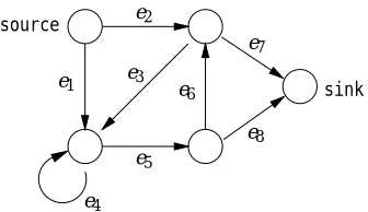
Figure 1: An example digraph. Edge ei receives input xi. The input vector x= (x1,...,x8) is expanded to the feature vector Φ(x) = (x2x7,x1x5x8,x2x3x5x8,x1x4x5x8,x1x5x6x7, x2x3x4x5x8,x2x3x5x6x7,x1x4x4x5x8,x1x5x6x3x5x8,...). The order of the features is arbi-trary but fixed.

case, x0_e=1 as well. The number of inputs n may be less than the number of edges, i.e. edges may share inputs. But in the simplest case (for example in Figure 1), n=|E(G)|and edge ei receives input xi.

The input vector x is expanded to a feature vector that has one feature for each source-to-sink path. The feature XPassociated with path P is the product of the inputs of its edges, i.e. XP=∏e∈Pxe (see Figure 1). (Throughout the paper, we use upper case letters for the product features and lower case letters for inputs.) We letΦ(x)be the vector of all path features. Given a second input vector x0on the edges, we define the path kernel of a directed graph as follows:

K(x,x0) =Φ(x)·Φ(x0) =

∑

∏

xex0e.

Similar related kernels that are built from regular expressions or pair-HMMs were introduced by Haus-sler (1999), Watkins (1999) for the purpose of characterizing the similarity between strings.

We would like to have efficient algorithms for computing kernels. For this reason we first generalize the definition to sums over all paths starting at any fixed vertex rather than the source. For any vertex u, let

P

Ku(x,x0) =

∑

∏

xe

∏

x0_e=

∑

∏

xex0e.

Clearly K_source(x,x0)gives the dot productΦ(x)·Φ(x0)that is associated with the whole graph G. For any vertex u other than the sink we have:

Ku(x,x0) =

∑

x₍u,u0)x0₍u,u0)Ku0(x,x0). (2.1)

The computation of K depends on the complexity of the graph G. If G is acyclic, then the functions Ku(x,x0)can be recursively calculated in a bottom up order using (2.1) and

Clearly this takes time linear in the number of edges.

When G is an arbitrary digraph (with cycles and infinite path sets), then (2.1) and (2.2) form a system of linear equations which can be solved by a standard method, e.g. Gaussian elimination. In this paper we only need the case when all inputs to the edges are non-negative and K(x,x0) is finite. For that case we show in Appendix A that the solution is unique. Alternatively Ku can be computed via dynamic programming using essentially the Floyd-Warshal all-pairs shortest path algorithm (Mohri, 1998). The cost of these algorithms is essentially cubic in the number of vertices of G. Speed-ups are possible for sparse graphs. A more efficient method is given later in Section 4.1 for the case when the graph, viewed as a DFA, has a concise regular expression.

3. A Hierarchically Constructed Digraph That Motivates the Subset Kernel

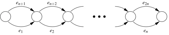
In this section we discuss the kernel associated with the digraph given in Figure 2 and use it as a motivating example for what is to follow in great detail in the next section. This kernel was the initial focal point of our research.

First observe that the paths of this graph can be described using the following simple regular expression

(e1+en₊1)(e2+en+2)...(en+e2n). (3.1) Assume the bottom edges ei receive input value xi and all top edges en₊i receive input one. The feature XP is the product of the inputs along the path P. So XP=∏i∈Axi, where A is the subset of indices in {1,...,n} corresponding to the bottom edges in P. If you now consider two input values xi and x0_i to the bottom edges, then Φ(x) and Φ(x0) have one feature for each of the 2n subsets/monomials over n variables, and the dot product defines a kernel

K(x,x0) =Φ(x)·Φ(x0) =

∑

∏

xix0i= n

∏

i=1

(1+xix0i). (3.2)

We call this the subset kernel.3 This kernel was introduced by Kivinen and Warmuth (1997) and is also sometimes called the monomial kernel (Khardon et al., 2001). Note that it computes a sum over 2n subsets in O(n) time and this computation is closely related to the above regular expres-sion: Replace ei by xix0_i, en₊i by xn+ix0n+i=1, the regular+by the arithmetic +, and the regular concatenation by the arithmetic multiplication. Also note that the fundamental unit in the graph of Figure 2 is a pair of vertices connected by a top and bottom edge. The whole graph may be seen as a “sequential composition” of n of such units.

We will use this kernel again in Section 9 to motivate an efficient algorithm for learning disjunc-tions. In the next section we discuss general schemes for building graphs and kernels from regular expressions.

4. Regular Expressions for Digraphs

Generalizing the above example, we consider a digraph as an automaton by identifying the source and the sink with the start and the accept state, respectively. The set of all source-sink paths is a

3. If the top edges receive inputs xn+i and x0n+i, respectively, then K(x,x0) =∑A⊆{1,...,n}∏i∈Axix0i∏i∈/Axn+ix0n+i=

∏n

en+1

e1 e2 en+2

en

e2n

Figure 2: The digraph that defines the subset kernel: The top edges receive input one and function asεedges.

regular language and can be expressed as a regular expression. For example the set of paths of the digraph given in Figure 1 is expressed as

e2e7+ (e1+e2e3)e∗₄e5(e6e3e∗₄e5)∗(e8+e6e7).

We assume in this paper that each edge symbol identifies a single edge and thus there is never any confusion about how words map to paths. Note that in the above regular expression some symbols appear more than once. So when we convert multiple occurrences of the same symbol to edges we use differently named edges for each occurrence but assign all of them the same input.

Since path features are products, the edges e that are always assigned the constant one (i.e. xe=1) function as theεsymbol in the regular expression. On the other hand, as we will see later, when we consider probabilistic weights on edges,εedges are not always assigned weight one.

The convolution kernel based on regular expressions was introduced by Haussler (1999). We will show that computing regular expression kernels is linear in the size of the regular expression that represents the given digraph G. Recall that the methods for computing kernels introduced in Section 2 take O(n3)time, where n is the number of vertices of G. So there is a speed-up when there is a regular expression of size O(n3_{). Even though the size of the smallest regular expression can be} exponential in n, we will see that there are small regular expressions for many practical kernels.

For the sake of simplicity we assume throughout the paper that the source has no incoming and the sink no outgoing edges (One can always add new source and sink vertices and connect them to the old ones viaεedges).

4.1 Series Parallel Digraphs

First let us consider the simple case where regular expressions do not have the∗-operation. In this case the prescribed graphs (corresponding to regular expressions with the operations union (+) and concatenation (◦)) are series parallel digraphs (SP digraphs, for short) (Valdes et al., 1982).

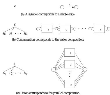
For a regular expression H, letH denote the SP digraph that H represents. Furthermore, we sometimes write H(s,t) to explicitly specify the source sand the sink t. Now we clarify how a regular expression with operations + and ◦ recursively defines a SP digraph (see Figure 3 for a schematic description). A symbol e defines the SP digraph H(s,t) consisting of a single edge with label e, initial vertex s and terminal vertex t. Let H1,...,Hk be regular expressions and

e e

(a) A symbol corresponds to a single edge.

H1 H2

◦

Hk

H1 H2 Hk

(b) Concatenation corresponds to the series composition.

H2

+

H1 Hk

Hk H1

H2

(c) Union corresponds to the parallel composition.

Figure 3: Regular expressions (as syntax trees on the left) and their corresponding SP digraphs (right).

the sinkti and the sourcesi+1are merged into one internal vertex. Finally, the union of the regu-lar expression H1,...,Hk, denoted by H=H1+···+Hk, corresponds to the parallel composition

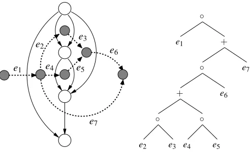
H(s,t)of the corresponding SP digraphsH1(s1,t1),...,Hk(sk,tk), where all sources are merged into the sourcesand all sinks are merged into the sinkt. In Figure 4 we give an example SP digraph with its regular expression (represented by a syntax tree).

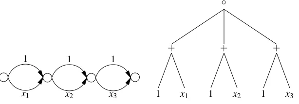
The syntax tree is used to compute the dot productΦ(x)·Φ(x0). We represent the feature vector Φ(x)by the syntax tree where the leaves e are replaced by their assignments xe. The feature vector Φ(x0) is the same except now the assignments x0_e are used. For computing the dot product, we replace the leaves labeled edge e by the input product xex0e, the union +by the arithmetic plus+ and the concatenation ◦ by the arithmetic multiplication ×. Now the value of the dot product is computed by a postorder traversal of the tree. This takes time linear in the size of the tree (number of edges). See Figure 5 for an example. For this figure, ei receives input xiand x0i, respectively.

e5 e3

e6 e4

e2

e1

e7

e2

+

+ +

e1

+ e7

e6

e3 e4 e5

◦

◦

Figure 4: An example of a SP digraph and its syntax tree.

x2

+

x1 ◦

+ x7

x6

◦

+ +

x3 x5

=

x4

+

x2x02 x1x01

x7x07

+

× x6x0₆

+

x5x05 x3x03x4x04

+

×

x0₂ x0₃ x0₄ x0₅ + +

◦ x0₆

x0₇ +

x0₁ ◦ +

Figure 5: The computation of dot productΦ(x)·Φ(x0): The trees on the left represent the feature vectorsΦ(x)and Φ(x0), respectively; the tree on the right represents the computation of the dot product, where the regular union+is replaced by the arithmetic+and the regular concatenation◦becomes the arithmetic multiplication×.

other words,

P

KH(x,x0) =ΦH(x)·ΦH(x0) =

∑

∏

xex0_e,

whereΦH(x)is the feature vector defined by a regular expression H with leaf assignments x. Now it is straightforward to see that this kernel is recursively calculated as follows:

KH(x,x0) =   

xex0e if H=e for some edge symbol e, ∏k

i=1KHi(x,x0) if H=H1◦ ··· ◦Hk, ∑k

i=1KHi(x,x0) if H=H1+···+Hk.

1

x2 x1

1

x2 x1

1

x2 x1

1

x2 x1

x2 1 x1

+

x2 1 x1

+

x2 1 x1

+

x2 1 x1

+

◦

Figure 6: Some inputs to distinct edges might be the same. The feature vector is Φ(x) =

(1,4x1,4x2,6x21,12x1x2,6x22,4x31,12x21x2,12x1x22,4x32,x14,4x31x2,6x21x22,4x1x32,x42). This de-fines the polynomial kernel K(x,x0) = (1+x·x0)4.

1

x2

1

x3 1

x1

+

1 x1

+

1

+

1 x3 x2

◦

Figure 7: One feature per subset of {1,2,3}: Φ(x) = (1,x1,x2,x3,x1x2,x1x3,x2x3,x1x2x3). This defines the subset kernel K(x,x0) =∏3_i=1(1+xix0i).

This is the path kernel defined by the regular expression

(e1_,0+e1,1+···+e1,n)(e2,0+e2,1+···+e2,n)···(ek,0+ek,1+···+ek,n),

where all edges e_∗,0receive input one, and all edges e∗,i(with i≥1) receive inputs xiand x0i, respec-tively. The tree in Figure 6 represents the feature vectorΦ(x)for the polynomial kernel with n=2 and k=4.

A related example is given in Figure 2 which is the digraph associated with the subset kernel (3.2). Now the bottom edges ei receive input values xi and x0_i, respectively, and the top edges en₊i always receive input one (see Figure 7: left). In this caseΦ(x) has one feature for each of the 2n subsets/monomials over n variables. The syntax diagram representing Φ(x) is given in Figure 7: right.

Since the inputs to the edges might not be distinct (see example in Figure 6), we can use short-hands for the union and concatenation of identical subgraphs that receive the same assignment. Specifically, letΦ(n◦)H(x)andΦ(n+)H(x)denote the feature vectors defined by the n-fold concate-nation and the n-fold union of H, respectively, with the same assignments x to its leaves (see Figure 8 for an example). Clearly,

+

x2 1 x1

4◦

Figure 8: Shorthand for identical subgraphs. This defines the same feature vector as in Figure 6.

and

K(n+)H(x,x0) =Φ(n+)H(x)·Φ(n+)H(x0) =nKH(x,x0).

In the table below we summarize the correspondence between regular operators and arithmetic operations.

regular arithmetic

◦ concatenation × multiplication

+ union + sum

n◦ n-fold concatenation ∧n power n n+ n-fold union ×n times n

4.2 Allowing∗-operations

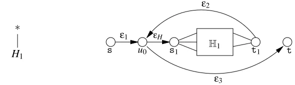
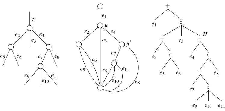
Now we consider the general case where regular expressions have∗-operations. First let us clarify how the digraph is defined by ∗-operations. LetH1(s1,t1) be any digraph that is defined by a regular expression H1. Then we define the digraph for H=H₁∗as in Figure 9: add a new sources, an internal vertex u0and a new sinkt, and connect withε-edges fromsto u0, fromt1to u0, from u0 totand from u0tos1. For convenience we call themε1,ε2,ε3and εH, respectively. The last edgeεH is called the repeat edge ofHand will play an important role. Note that theε-edges are newly introduced and there are no such symbols in the given regular expression H=H₁∗. Actually we can eliminate theε-edges by merging the five verticess, u0,s1,t1 andtinto one vertex. We introduce the dummyε-edges for the following three reasons.

∗

H1 H1

ε1

u0 s1

ε3

t1 t

s

ε2

εH

1. The properties thatshas no incoming edges andthas no outgoing edges are preserved.

2. There remains a one-to-one correspondence between the set of paths in the componentHand the language that the regular expression H produces. In particular, the trajectory of a path P inHexcludingεtransitions forms a symbol sequence that H produces.

3. As we will see later, the kernel computation and weight updates for H1can be made indepen-dent of the larger component.

The kernel KH(x,x0) =∑P∈PH∏_e∈Pxex0_e can be calculated as before by traversing the syntax

tree (now with operations+,◦and∗) in postorder. The local operation done when completing the traversal of a∗-node is as follows: When H=H₁∗for some regular expression H1, then

KH(x,x0) =x_ε1x0_ε1

∞

∑

k=0

x_εHx0εHK

H1(_x,_x0)_x

ε2x0_ε2kx_ε3x0_ε3 = xε1x

0 ε1xε3x0_ε3 1−x_εHx0_εHx_ε2x0_ε2KH1(_x,_x0)

if xεHx0εHxε2x 0

ε2KH1(x,x0)<1 and KH(x,x0) =∞otherwise.

5. Using Path Kernels to Represent Weights

In this paper we describe algorithms that use the path weights as linear weights. The direct represen-tation of the weights is the weight vector W which has one component WP per path P. The indirect representation of the weights is a weight vector w on the edges for which W =Φ(w). If the graph has cycles, then the dimension of W is countably infinite, and in the acyclic case the dimension of W is typically exponential in the dimension of w.

The predictions of the algorithms are determined by kernel computations. In the simplest case there is a set of inputs xe to the edges and path P predicts with XP =∏e∈Pxe. The algorithm combines the predictions of the paths by predicting with the weighted average of the predictions of the paths or with a squashing function applied on top of this average. A typical squashing function is a threshold function or a sigmoid function. The weighted average becomes the following dot product:

∑

P

WPXP=

∑

∏

we !

∏

e∈P xe

!

=Φ(w)·Φ(x) =K(w,x).

In a slightly more involved case, the prediction of path P is the sum of the predictions of its edges, i.e.∑_e∈Pxe. Now the weighted average can be rewritten as

∑

P WP

∑

e∈P

xe=

∑

P e

∑

∏

!

xe=

∑

xe

∑

∏

we0 !

I(e∈P), (5.1)

where I(true) =1 and I(false) =0. For edge e, let uebe edge weights defined as

ue_e0 =

1 if e06=e, 0 if e0=e.

Then, we can see that

I(e∈P) =1−

∏

By plugging this into the r.h.s. of (5.1) we can again rewrite the weighted average using kernel computations:

∑

P WP

∑

e∈P

xe=

∑

xe

∑

∏

we0−

∏

e0∈P we0ue_e0

!

=

∑

e∈E(G)

xe(K(w,1)−K(w,ue)), (5.2)

where 1 denotes the vector whose components are all 1. As before, the prediction of the algorithm might be a squashed version of this average.

5.1 Probabilistic Weights

We will use the path kernel to represent a probabilistic weight vector on the paths, i.e. W =Φ(w)is a probability vector. Thus we want three properties for the weights on the set of paths (by default, all weights in this paper are non-negative):

P1 The weights should be in product form. That is,

WP=

∏

we,

where weare edge weights.

P2 The outflow from each vertex u should be one. That is, for any vertex u of G,

∑

u0:(u,u0)∈E(G)

w₍u,u0)=1,

where E(G)denotes the set of edges of G.

P3 The total path weight is one. That is,

∑

P

WP=1.

Note that the sum of Property P3 is over all paths of G from the source to the sink. The three prop-erties make it trivial to generate random paths: Start at the source and iteratively pick an outgoing edge from the current vertex according to the prescribed edge probabilities until the sink is reached. Property P3 guarantees that any random walk eventually goes to the sink. In other words, any vertex u that is reachable from the source via a (partial) path of non-zero probability must also reach the sink via such a path.

5.2 Decomposable Multiplicative Updates

In this paper we restrict ourselves to updates that multiply each edge weight by a factor and then the total weight of all paths is renormalized. Let WP be the old weight for path P and ˜WP the updated weight. Assume that the old weights are in product form, i.e. WP=∏e∈Pweand let bebe the update factor for edge e. Then updates must have the following form:

˜ WP=

WP∏e∈Pbe ∑PWP∏e∈Pbe =

∏e∈Pwebe

Φ(w)·Φ(b). (5.3)

The normalization needs to be non-zero and finite. That is, we need the following property on the edge factors be:

P4 The edge factors beare non-negative and

0<

∑

WP

∏

be<∞.

Typically, the edge factors satisfy 0<be<1, and in this case Property P4 is satisfied.

Note that the updated weights are not in product form any more. In the next section we will give an algorithm that translates the above update (5.3) into an update of the edge weights so that the new weights again have the product form and satisfy Properties P1–3 again. In this section we discuss (at a high level) general update families that give rise to updates of the above form.

Consider the following update on the path weights

˜ WP=

WPexp(−η`P) ∑PWPexp(−η`P),

(5.4)

whereηis a non-negative learning rate and`Pis the loss of path P in the current trial. This is known as the loss update of the expert framework for on-line learning, where the paths are the experts. One weight is maintained per expert/path and the weight of each expert decays exponentially with the loss of the expert. The Bayes Update can be seen as a special case, when the loss is the log loss (DeSantis et al., 1988). Another special case is the Weighted Majority algorithm (Littlestone and Warmuth, 1994) (discrete loss). General loss functions were first discussed in the seminal work of Vovk (1990). See Kivinen and Warmuth (1999) for an overview.

The loss update has the required form (5.3), if`P decomposes into a sum over the losses le of the edges of P, i.e.

`P=

∑

leand be=exp(−ηle). (5.5)

For maintaining Property P4, it is sufficient to assume that for all paths P, the losses`P are both upper and lower bounded. The applications of Sections 7, 8 and 10 use the loss update, where the loss of a path decomposes into a sum. In many cases, however, the loss does not decompose into a sum. In Section 9, we discuss this issue in the context of learning disjunctions.

The loss update is a special case of the Exponentiated Gradient (EG) update (Kivinen and War-muth, 1997), which is of the form

˜

WP=WPexp

−η_∂∂λ

WP

whereλis the current loss of the algorithm (which depends on the weights W ) and Z renormalizes the weights to one. Ifλ=∑PWP`P, then <sub>∂</sub>∂λ<sub>WP</sub> =`P, and the EG update becomes the loss update (5.4).

So to obtain EG updates of the required form (5.3), we want the gradient of the loss to decom-pose into a sum over the edges. The canonical case is the following. Assume that inputs x are given to the edges, the prediction of a path P is∑e∈Pxe, and the prediction of the algorithm is given by

ˆ

y=σ(aˆ),where ˆa=

∑

WP

∑

xe (5.7)

and σ(.) is a differentiable squashing function (Recall that we showed in (5.2) how to write the weighted path prediction ˆa as a sum of kernel computations.) Assume the loss λ measures the discrepancy between the prediction ˆy and a target label y. That is,λ=`(y,yˆ), where`is a function

R

R

R

˜

WP=WPexp −ηλ0

∑

xe !

/Z, (5.8)

where

λ0₌ ∂`(y,σ(a))

∂a

a=aˆ

.

For example, in the case of the square loss,4 we have λ0 =2σ0(aˆ)(yˆ−y). Since the derivative λ0 is constant with respect to P, the exponent decomposes into a sum over the edges. Thus in this canonical case, the EG update (5.8) has the required form (5.3), where the edge factors are

be=exp −ηλ0xe. (5.9)

In Section 9 we will use this form of the EG update for designing efficient disjunction learning algorithms. The discrete loss for disjunctions does not decompose into a sum. However by using a prediction of the form (5.7) and an appropriate loss function for our algorithm, we are in the lucky situation where the gradient of this loss decomposes into a sum and our efficient methods are again applicable.

The term “multiplicative update” is an informal term where each updated weight is proportional to the corresponding previous weight times a factor. A more precise definition is in terms of the regularization function used to derive the updates: Multiplicative updates must be derivable with a relative entropy or an unnormalized relative entropy as the regularization (see Kivinen and Warmuth 1997 for a discussion, where these update are called EG and EGU updates, respectively). The Unnormalized Exponentiated Gradient (EGU) update has the same form as the EG update (5.6) except that the weights are not normalized.

Note that for the methodology of this paper, the update must have form (5.3), and if the algorithm uses a prediction, then it must be efficiently computable via for example kernel computations.

6. Weight Pushing Algorithm

The additional factors b on the edges (from the multiplicative update (5.3)) mess up the three Prop-erties P1–3. However there is an algorithm that rearranges the weights on the edges so that the relative weights on the path remain unchanged but again have the three properties. This algorithm is called the Weight Pushing algorithm developed by Mehryar Mohri (1998) in the context of speech recognition.

The generalized path kernels Kuwill be used to re-normalize the path weights with the Weight Pushing algorithm. Assume that the edge weights we and the path weights WP fulfill the three Properties P1–3. Our goal is to find new edge weights ˜weso that the three properties are maintained. A straightforward way to normalize the edge weights would be to divide the weights of the edges leaving a vertex by the total weight of all edges leaving that vertex. However this usually does not give the correct path weights (5.3) unless the product of the normalization factors along different paths is the same. Instead, the Weight Pushing algorithm (Mohri, 1998) assigns the following new weight to the edge e= (u,u0):

˜

we=webeKu0(w,b) Ku(w,b)

. (6.1)

Below we show that the three properties are maintained for the updated weights ˜WPand ˜we.

Theorem 1 Assume that the path weights W and the edge weights w fulfill the three Properties P1,

P2 and P3. Let ˜WPbe the updated path weight given by (5.3) and ˜webe the new edge weights given by (6.1). Here we assume that Property P4 holds. Then, ˜W and ˜w fulfill the three Properties P1, P2 and P3.

Proof Property P3 follows from the definition (5.3) of ˜WP. Here Property P4 is needed to assure that the normalization is positive. From (2.1), it is easy to see that the new weights ˜we are normalized, i.e. Property P2 holds for any non-sink vertex u,

∑

u0:(u,u0)∈E(G) ˜

w₍u,u0)=1.

Finally, Property P1 is proven as follows: Let P={(u0,u1),(u2,u3),...,(uk₋1,uk)} be any path from the source u0to the sink uk. Then by starting from (5.3) we get

˜ WP =

WP∏e∈Pbe ∑PWP∏e∈Pbe

= ∏e∈Pwebe K_source(w,b)

= ∏e∈PwebeKsink(w,b) K_source(w,b)

=

∏

i=1

w₍ui−1,ui)b(ui−1,ui)Kui(w,b)

Kui−1(w,b)

=

∏

Recall that in Section 4 we showed how to speed-up the kernel computation when the digraph is represented as a regular expression. In Appendix C we will implement the Weight Pushing algorithm on syntax diagrams for regular expression. The first algorithm is linear in the size of the regular expression. We then give sub linear algorithms for computing the dot productΦ(w)·Φ(x) when most of the xeare one, and for implementing the Weight Pushing algorithm when most of the factors beare one.

Before we begin with applications of our methods in the next section, we describe the Weight Pushing algorithm for the subset kernel given in Section 3: See regular expression (3.1) and the digraph of Figure 2. This example might give an idea how the Weight Pushing algorithm can be implemented on regular expressions. Assume that the factors ben+i are all one. By Property P2 we

have wen+i =1−wei. So each pair of edges ei and en+i contributes a factor 1−wei+weibei in the

kernel computation (see the footnote of p. 777). More generally, if uj is the vertex at which the j-th pair is starting, then

Kuj(w,b) =

∑

P∈P(uj)

∏

e∈P webe=

n

∏

i=j

(1−wei+weibei).

With this we see that the ratio of kernels in (6.1) cancel, except for the factor belonging to the j-th pair, and

˜

wej =wejbej/(1−wej+wejbej)and ˜wen+j = (1−wej)/(1−wej+wejbej). (6.2)

This re-normalization of the weights will be used in the BEG algorithm for learning disjunctions (Section 9).

7. A Dynamic Routing Problem

In the subsequent sections we show various applications of our method. In particular, in this and the next sections we discuss two on-line network routing problems. Assume that we want to send packets from the source to the sink (destination) of a given digraph (network). For each trial t, we assign transition probabilities wt_,e to the edges that define a probabilistic routing. Starting from the source we choose a random path P to the sink according to the transition probabilities and try to send the packet along the path. But some edges (links) may be very slow due to network congestion. The goal is to find a protocol that is competitive with the optimal static routing chosen in the hindsight. Note that we make no assumptions on how the traffic changes in time. In other words we seek guarantees that hold for arbitrary network traffic. There are several ways to define the “resistance” of an edge as well as the throughput of a protocol. In this section, the resistance is the success probability of transferring the packet along the edge, and the throughput of a protocol is measured by the total success probability of sending all packets from the source to the sink. In the next section, the resistance and the throughput are defined in terms of the time it takes for a packet to traverse a link rather than the success probability.

our model are new and may be more appropriate for networks operating in a strongly adversarial environment. Below we give the problem formally.

In each trial t=1,2,... ,T , the following happens:

1. At the beginning of the trial, the algorithm has transition probabilities wt_,e∈[0,1]for all edges e, such that Properties P1–3 hold.

2. Conductances dt,e∈[0,1]for all edges are given. Let Xt denote the event that the current packet is successfully sent from the source to the sink. Assuming independence between con-ductances of individual edges, the probability that the current packet is sent along a particular path P becomes

Pr(Xt|X1,...,Xt−1,P) =

∏

dt,e. (7.1)

3. A random path P is chosen with probability Wt,P=∏e∈Pwt,e. The success probability at this trial is

at =

∑

Wt,PPr(Xt|X1,...,Xt−1,P) =Φ(wt)·Φ(dt).

4. The path weights Wt,P are updated indirectly to Wt+1,P by updating the edge weights wt,e to wt₊1,e, while maintaining Properties P1–3.

The goal is to make the total success probability∏_tT₌₁at as large as possible.

In the feature space we can employ the Bayes algorithm. The initial weights are interpreted as a prior for path P, i.e. Pr(P) =W1_,P =∏e∈Pw1,e. We assume that the initial edge weights w1,e are chosen so that Properties P1–3 are satisfied and W1,P>0 for all paths P. Then the Bayes algorithm sets the weight Wt₊1,P as a posterior of P given the input packets X1,...,Xt observed so far. Specifically, assuming Wt_,P =Pr(P|X1...Xt−1), then the Bayes algorithm updates the path weights as

Wt+1,P = Pr(P|X1,...,Xt)

= Wt,PPr(Xt|X1,...,Xt−1,P) ∑PWt,PPr(Xt |X1,...,Xt−1,P)

= Wt,P∏e∈Pdt,e ∑PWt,P∏e∈Pdt,e.

(7.2)

Here we assume that at least one static routing P has positive success probability, i.e., Pr(X1,...,XT| P)>0. This assumption implies that Property P4 holds and the denominator of (7.2) is always positive. Note that this update has the required form (5.3), where the dt_,efunction as update factors to the edges. Thus the Weight Pushing algorithm can be used to update the edge weights wt_,e to wt+1,e. Below we show that the Bayes algorithm achieves the best possible competitive ratio against the optimal static routing.

Theorem 2 The Bayes algorithm guarantees the following performance.

T

∏

t=1

at=

∑

W1_,PPr(X1,...,XT |P)≥max

On the other hand, for any protocol there exist conductances such that

T

∏

t=1

at ≤max

P W1,PPr(X1,...,XT |P).

Proof First we analyze the throughput of the Bayes algorithm. Repeatedly applying Bayes rule, we

have

T

∏

t=1 at =

T

∏

t=1

Pr(X1,...,Xt) Pr(X1,...,Xt₋1)=

∑

W1,PPr(X1,...,XT |P), which implies the first part of the theorem.

Next we consider a strategy for the adversary. Fix a simple path P∗arbitrarily, and for any trial t, let dt,e=1 if e∈P∗and dt,e=0 otherwise. Then, since at =Wt,P∗ for any t, we have

T

∏

t=1 at =

T

∏

t=1

Wt,P∗≤W1,P∗ =max

P W1,PPr(X1,...,XT |P).

Note that the bound ∑_PW1,PPr(X1,...,XT |P)for the Bayes algorithm is usually much larger than that for the static routing with the initial prior, which is expressed as ∏T_t=1∑_PW1,PPr(Xt | X1,...,Xt₋1,P). For example, consider the conductances used to show the lower bound of the above theorem. In this case, the Bayes algorithm has constant bound W1,P∗, whereas the static routing has exponentially smaller bound W₁T_,P∗.

Note that in this simple example, the algorithm did not produce a prediction in each trial. How-ever, note that the success probability can be expressed as a kernel computation. Also, if we define the loss of path P at trial t as`t,P=−ln Pr(Xt|X1...Xt−1,P), then by (7.1) this loss decomposes into a sum over the edges, i.e. `t,P=∑e∈P−ln(dt,e). Now, for learning rateη=1, Bayes rule (7.2) be-comes an example of a decomposable loss update (5.4), (5.5), where the independence assumption on the acceptance probabilities of the edges (7.1) caused the negative log likelihood to decompose into a sum.

8. On-line Shortest Path Problem

In this section we let dt,e denote the time it takes the t-th packet to travel along the edge e. The throughput of a protocol is measured by the total amount of time it takes to send all packets from the source to the sink. Equivalently, we can interpret dt,e as the distance of edge e at trial t. Our overall goal is to make the total length of travel from the source to the sink not much longer than the shortest path of the network based on the cumulative distances of all packets for each edge. We call this problem the on-line shortest path problem. We prove a bound for an algorithm and then return to the digraph that defines the subset kernel. For this type of graph there is an improved bound. For our bounds to be applicable, we require in this section that the digraph G defining the network is acyclic. This assures that all paths have bounded length.

In each trial t=1,2,... ,T , the following happens:

2. Distances dt_,e∈[0,1]for all edges are given.

3. The algorithm incurs a lossλt which is defined as the expected length of path of G. That is,

λt =

∑

Wt,P`t,P,

where

`t,P=

∑

dt,e (8.1)

is the length of the path P, and this is interpreted as the loss of P.

4. The path weights Wt_,P are updated indirectly to Wt+1,P by updating the edge weights wt,e to wt+1,e, respectively, while maintaining Properties P1–3.

Note that the length`t,Pof path P at each trial is upper bounded by the number of edges in P. Letting D denote the depth (maximum number of edges of P) of G, we have`t,P∈[0,D]. Note that the path P minimizing the total length

T

∑

t=1

`t,P= T

∑

t=1e

∑

dt,e=

∑

T

∑

t=1 dt,e

can be interpreted as the shortest path based on the cumulative distances of edges: ∑T_t=1dt_,e. The goal of the algorithm is to make its total loss∑T_t=1λt not much larger than the length of the shortest path.

Considering each path P as an expert, we can view the problem above as a dynamic resource al-location problem introduced by Freund and Schapire (1997). So we can apply their Hedge algorithm which is a reformulation of the Weighted Majority algorithm (see WMC and WMR of Littlestone and Warmuth, 1994). Let W1,P =∏e∈Pw1,e be initial weights for paths/experts. Note that since the graph is acyclic with a unique sink vertex, the initial weights W1_,Psum to 1 and Property P3 is satisfied. At each trial t, when given losses`t,P∈[0,D]for paths/experts, the algorithm incurs loss

λt =

∑

Wt,P`t,P

and updates weights according to

Wt+1,P=

Wt,Pβ`t,P/D ∑P0Wt,P0β`t,P0/D

, (8.2)

For the rest of this section we discuss bounds that hold for the Hedge algorithm. It is shown by Littlestone and Warmuth (1994) and Freund and Schapire (1997) that for any sequence of loss vectors for the experts, the Hedge algorithm guarantees5 that

T

∑

t=1

λt≤min P

ln(1/β) 1−β

T

∑

t=1

`t,P+ D 1−βln

1 W1,P

!

. (8.3)

Below we give a proof of (8.3) with a more sophisticated form of the bound.

Fix an arbitrary probability vector U on the paths. Let d(U,Wt) =∑PUPln(UP/Wt,P)denote the relative entropy between U and Wt. Looking at the progress d(U,Wt)−d(U,Wt+1)for one trial, we have

d(U,Wt)−d(U,Wt+1) =

∑

UPln(Wt₊1,P/Wt,P)

=

∑

P

UPln β

`t,P/D

∑P0Wt,P0β`t,P0/D

= lnβ

D

∑

∑

`t,P/D.

Since `t,P/D∈[0,1]and 0≤β<1, we have β`t,P/D≤1−(1−β)`t,P/D. Plugging this into the second term, we have

ln

∑

Wt_,Pβ`t,P/D ≤ ln 1−(1−β)

∑

Wt_,P`t,P/D !

= ln(1−(1−β)λt/D)

≤ −(1−β)λt/D.

Thus

d(U,Wt)−d(U,Wt+1)≥ lnβ

D

∑

D λt.

Summing this over all t’s we get

d(U,W1)≥d(U,W1)−d(U,WT+1)≥ lnβ

D

∑

∑

t=1

`t,P+ 1−β

D T

∑

t=1 λt,

or equivalently,

T

∑

t=1 λt ≤

ln(1/β) 1−β

∑

T

∑

t=1

`t,P+ D

1−βd(U,W1). (8.4)

If U is the unit vector that attains the minimum of the right hand side, we have (8.3).

8.1 Improved Bounds for Hierarchically Constructed Digraphs

Unfortunately, the loss bound (8.4) depends on the depth D of G. Thus for graphs of large depth or for cyclic graphs, the bound is vacuous. In some cases, however, we can prove bounds where the depth D is replaced with a much smaller depth than the depth of the entire graph G.

Theorem 3 Assume that a graph G is a series composition of acyclic digraphs H1,...,Hn. Note that each component graph Hiis not necessarily a SP digraph. Let D be the maximum depth of a component. Then, the Hedge algorithm using the update rule (8.2) guarantees that

T

∑

t=1 λt ≤

ln(1/β) 1−β

∑

T

∑

t=1

`t,P+ D

1−βd(U,W1).

Proof We use the convention thatΦHi(_x)_{denotes the feature vector based on the paths of H}

i. As in the case of SP digraphs, we have

Φ(wt)·Φ(bt) = n

∏

i=1

ΦHi(_wt)·ΦHi(_bt),

where bt_,e=βdt,e/D. Therefore

ln

∑

Wt,Pβ`t,P/D = lnΦ(wt)·Φ(bt)

=

∑

i=1

lnΦHi(_w

t)·ΦHi(bt)

=

∑

i=1

ln

∑

P∈PHi

Wt_,Pβ`t,P/D

≤

∑

i=1

−(1−β)λt,i/D

= −(1−β)λt/D,

whereλt,i=∑P∈PHiWt,P`t,Pis the expected length of the partial paths through Hiandλt =∑ni=1λt,i. Using the same technique as in the previous proof, we get the theorem.

For example, let us return to the digraph that defines the subset kernel (Figure 2). The graph is a series composition of n two-vertex graphs, where there are two parallel edges connecting the pairs of vertices. Note that although the depth of the whole graph is n, each component graph has depth constant one. So, the Hedge update (8.2) with D=1 leads to a bound that does not depend on the depth of the entire graph.

9. Learning Disjunctions and Conjunctions

decomposes into a sum lets us apply the path kernel methodology introduced in this paper. By choosing an appropriate digraph for each case, the weight pushing algorithm realizes all known effi-cient algorithms for learning disjunctions. The price for the gained efficiency is a slight degradation of the mistake bounds.

At each trial a binary instance vector xt ∈ {0,1}n is given to the algorithm. After the algorithm produces a binary prediction ˆyt, it receive a binary label yt and incurs discrete loss |ytˆ −y|(also binary). The goal is to design algorithms whose loss (or number of prediction mistakes) is not much worse than the loss of the best conjunction or disjunction of a given size k, where k is typically much smaller than the number of variables n. The Winnow algorithm was the first efficient algorithm for learning disjunction (Littlestone, 1988). Here we motivate two alternate algorithms and also briefly discuss Winnow. All these algorithms spend O(n)time to predict and update their weights and their loss bounds grow linearly in k and logarithmic in n.

We begin by discussing an algorithm for learning conjunctions. Recall the subset kernel of Kivinen and Warmuth (1997) introduced in Section 3 (the path kernel associated with Figure 2). Assume that the bottom edge ei receive input xt,i and the top edges en+i all receive input one and function as ε edges. Each path feature Xt_,P is the product over the inputs along the path. More precisely, Xt,P=Xt,A=∏i∈Axt,i, where A is the subset of indices in{1,...,n}corresponding to the bottom edges of P. So the subset feature Xt,A predicts as the conjunction over the variables with indices in A and|y−Xt_,A|is the discrete loss of conjunction A on the example(xt,yt).

One approach is to maintain a weight Wt_,A per subset A and predict with ˆyt =σθ(at), where at=∑AWt,AXt,Aandσθ(.)is the{0,1}-valued threshold function with thresholdθ. Here we choose θ=1/2. Assume the weights are updated multiplicatively using the loss update, i.e.

Wt+1,A=

Wt_,Aexp(−η|yt−Xt,A|))

Zt ,where Zt normalizes the total weight to 1.

Since the loss function is the discrete loss, this is an application of the Weighted Majority algo-rithm (Littlestone and Warmuth, 1994). Using methods similar to what was used in Section 8, it is easy to prove6 a mistake bound of O(k ln n+m∗), where m_∗is the number of mistakes of the best conjunction of size k.

Unfortunately, the algorithm is inefficient since it maintains 2n weights. Moreover, it was es-sentially shown by Khardon, Roth, and Servedio (2001) that computing the predictions for this type of update7is #P-hard. Our efficient methods do not apply because the discrete loss|yt−∏i∈Axt,i| does not decompose into a sum.

So how do we obtain an efficient learning algorithm for conjunctions? One way is to use additive algorithms such as the Perceptron algorithm together with the subset kernel. The additive algorithms for solving the same problem are efficient, but the bounds are much weaker (linear in n instead of logarithmic) (see discussion by Kivinen and Warmuth 1997, Kivinen et al. 1997, Khardon et al. 2001).

We now develop efficient multiplicative algorithms. For convenience, let us switch to learning disjunctions (Because of de Morgan’s law, the learning problems for conjunctions and disjunctions

6. Choose the prior W1,Aso that for each size, the total weight of all conjunction of that size is 1/n.

ˆ a ˆ

a

(1) y=0 (2) y=1

θ θ

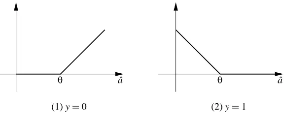
Figure 10: The hinge lossλ=|y−σ_θ(aˆ)| |θ−aˆ|as functions of ˆa.

are equivalent.) Now the loss of disjunction A on example(xt,yt)becomes

`t,A=|yt−I(

∑

xt_,i≥1)|,

where I(true) =1 and I(false) =0. Again, this discrete loss does not decompose and we cannot implement the loss update efficiently.

However, we now modify our setup. We let each disjunction predict with ∑i∈Axt,i instead of I(∑_i∈Axt,i≥1). The weighted average prediction is now ˆat =∑AWt,A∑i∈Axt,i and the algorithm predicts with ˆyt =σθ(aˆt), where the thresholdθis suitably chosen. For a moment let us assign the following loss to the algorithm

λt =|yt−σθ(atˆ)| |θ−atˆ|=`(yt,ytˆ).

So when ˆyt =yt, then this loss is zero. But when yt 6=ytˆ, it is linear in ˆat. This is the linear hinge loss used for motivating Support Vector Machines (Cristianini and Shawe-Taylor, 2000, Gentile and Warmuth, 1998). See Figure 10 to see how the hinge loss behaves with respect to the linear activation ˆat. Note that the weighted average prediction ˆat and the hinge lossλt are of the canonical form we discussed in Section 5.2. So the derivative ∂λt

∂Wt,A =λ 0

t∑i∈Axt,i decomposes into a sum with λ0

t= ∂`(yt,σθ(aˆ)/∂aˆ|aˆ=aˆt =ytˆ −yt (see Figure 10), and the EG update (5.8) has the required form

(5.3), with bt_,e=exp(−η(ytˆ −yt)xt,e). Now we can indirectly represent the weight vector Wt for the 2nsubsets by maintaining a weight vector wt on the 2n edges, so that Wt=Φ(wt)whereΦ(.)is the feature map of the subset kernel. We efficiently update the weights wt using the Weight Pushing algorithm on the digraph of Figure 2 (See update (6.2) and discussion at the end of Section 6). The weighted average ˆat can be expressed in term of kernel computations (5.2). However, for the the special case of the subset kernel it follows from (5.1) that ˆat =∑iwt,ei·xt,i. Hence the prediction

ˆ

yt is easy to compute. The algorithm described above is called the Binary Exponentiated Gradient algorithm (BEG algorithm, for short) for learning disjunctions (Bylander, 1997, Helmbold, Panizza, and Warmuth, 2002).

the form O(k ln n+a_∗). This includes BEG when the thresholds and learning rate is appropriately chosen (see Theorem 5 of Helmbold et al. 2002). Note that a_∗might be up to a factor of k larger than m_∗. So there is a price we have to pay for moving from the discrete loss to the decomposable hinge loss which leads to the more efficient algorithms.

The hinge loss can also be used to derive the normalized Winnow algorithm.8 However now a slightly different kernel must be used corresponding to the regular expression

(e1,1+e1,2+...e1,n)(e2,1+e2,2+...e2,n)...(en,1+en,2+...en,n),

where the edges e_∗,i receive input xi (i.e. xe_∗,i =xi). A path P={e1,i1,e2,i2,...,en,in}corresponds

to the disjunction with index set {i1,i2,...,in}. Note that now many paths represent the same disjunction. We follow the same derivation as for BEG. Instead of letting path P predict with I(∑e∈Pxt,e≥1)and using the discrete loss

`t,P=|yt−I(

∑

xt,e≥1)|,

we use a different prediction and the hinge loss. We let the path P predict with∑n_e∈Pxt,e, and use the loss

λt=|yt−σθ(atˆ)| |θ−atˆ|,where ˆat=

∑

Wt_,P

∑

xt_,e.

Again the loss decomposes. Assume that all edges ej,iare assigned the same initial weight w1,ej,i =

1/n. Then, since for any trial t all edges e_∗,ireceive the same factor bt,e∗,i =exp(−η(yˆ−y)xt,i), the

Weight Pushing algorithm keeps their weights wt,e∗,i the same. Let wt,i denote these weights. Now

the Weight Pushing algorithm updates the weights as follows:

wt+1,i=

wt,ibt,i ∑n

j=1wt,jbt,j,

where bt,i=exp(−η(yˆ−y)xt,i).

Also the prediction simplifies to the following:

ˆ

at = n

∑



wt,ixt,i

∑

wt,j

!n−1

 (9.1)

= n

∑

i

wt_,ixt_,i,

because∑jwt,j=1 for Normalized Winnow. The constant n can be incorporated into the threshold. See Theorem 9 of Helmbold et al. (2002) for the settings of the learning rate and threshold that lead to the O(k log n+a_∗) bound for Normalized Winnow, where a_∗ is as before the minimum number of bits/attributes that have to be flipped in all examples(xt,yt), so that there is a disjunction of size k that agrees with all labels yt.

The Winnow algorithm can also be derived using the hinge loss and the same kernel as Normal-ized Winnow. The only difference is that the weights are not normalNormal-ized and the Weight Pushing algorithm is not needed. However now, we do not know how to motivate the prediction of the Winnow algorithm because (9.1) does not simplify (since∑iwt,imight not be one).