Differentially Private Empirical Risk Minimization
Kamalika Chaudhuri [email protected]
Department of Computer Science and Engineering University of California, San Diego
La Jolla, CA 92093, USA
Claire Monteleoni [email protected]
Center for Computational Learning Systems Columbia University
New York, NY 10115, USA
Anand D. Sarwate [email protected]
Information Theory and Applications Center University of California, San Diego
La Jolla, CA 92093-0447, USA
Editor: Nicolas Vayatis
Abstract
Privacy-preserving machine learning algorithms are crucial for the increasingly common setting in which personal data, such as medical or financial records, are analyzed. We provide general techniques to produce privacy-preserving approximations of classifiers learned via (regularized) empirical risk minimization (ERM). These algorithms are private under theε-differential privacy definition due to Dwork et al. (2006). First we apply the output perturbation ideas of Dwork et al. (2006), to ERM classification. Then we propose a new method, objective perturbation, for privacy-preserving machine learning algorithm design. This method entails perturbing the objective function before optimizing over classifiers. If the loss and regularizer satisfy certain convexity and differentiability criteria, we prove theoretical results showing that our algorithms preserve privacy, and provide generalization bounds for linear and nonlinear kernels. We further present a privacy-preserving technique for tuning the parameters in general machine learning algorithms, thereby providing end-to-end privacy guarantees for the training process. We apply these results to produce privacy-preserving analogues of regularized logistic regression and support vector machines. We obtain encouraging results from evaluating their performance on real demographic and benchmark data sets. Our results show that both theoretically and empirically, objective perturbation is superior to the previous state-of-the-art, output perturbation, in managing the inherent tradeoff between privacy and learning performance.
Keywords: privacy, classification, optimization, empirical risk minimization, support vector
ma-chines, logistic regression
1. Introduction
violating their privacy. Thus, an emerging challenge for machine learning is how to learn from data sets that contain sensitive personal information.
At the first glance, it may appear that simple anonymization of private information is enough to preserve privacy. However, this is often not the case; even if obvious identifiers, such as names and addresses, are removed from the data, the remaining fields can still form unique “signatures” that can help re-identify individuals. Such attacks have been demonstrated by various works, and are possible in many realistic settings, such as when an adversary has side information (Sweeney, 1997; Narayanan and Shmatikov, 2008; Ganta et al., 2008), and when the data has structural properties (Backstrom et al., 2007), among others. Moreover, even releasing statistics on a sensitive data set may not be sufficient to preserve privacy, as illustrated on genetic data (Homer et al., 2008; Wang et al., 2009). Thus, there is a great need for designing machine learning algorithms that also preserve the privacy of individuals in the data sets on which they train and operate.
In this paper we focus on the problem of classification, one of the fundamental problems of machine learning, when the training data consists of sensitive information of individuals. Our work addresses the empirical risk minimization (ERM) framework for classification, in which a classifier is chosen by minimizing the average over the training data of the prediction loss (with respect to the label) of the classifier in predicting each training data point. In this work, we focus on regularized ERM in which there is an additional term in the optimization, called the regularizer, which penalizes the complexity of the classifier with respect to some metric. Regularized ERM methods are widely used in practice, for example in logistic regression and support vector machines (SVMs), and many also have theoretical justification in the form of generalization error bounds with respect to independently, identically distributed (i.i.d.) data (see Vapnik, 1998 for further details).
For our privacy measure, we use a definition due to Dwork et al. (2006b), who have proposed a measure of quantifying the privacy-risk associated with computing functions of sensitive data. Their
ε-differential privacy model is a strong, cryptographically-motivated definition of privacy that has
recently received a significant amount of research attention for its robustness to known attacks, such as those involving side information (Ganta et al., 2008). Algorithms satisfyingε-differential privacy are randomized; the output is a random variable whose distribution is conditioned on the data set. A statistical procedure satisfiesε-differential privacy if changing a single data point does not shift the output distribution by too much. Therefore, from looking at the output of the algorithm, it is difficult to infer the value of any particular data point.
In this paper, we develop methods for approximating ERM while guaranteeing ε-differential privacy. Our results hold for loss functions and regularizers satisfying certain differentiability and convexity conditions. An important aspect of our work is that we develop methods for end-to-end
privacy; each step in the learning process can cause additional risk of privacy violation, and we
provide algorithms with quantifiable privacy guarantees for training as well as parameter tuning. For training, we provide two privacy-preserving approximations to ERM. The first is output
per-turbation, based on the sensitivity method proposed by Dwork et al. (2006b). In this method noise
is added to the output of the standard ERM algorithm. The second method is novel, and involves adding noise to the regularized ERM objective function prior to minimizing. We call this second method objective perturbation. We show theoretical bounds for both procedures; the theoretical performance of objective perturbation is superior to that of output perturbation for most problems. However, for our results to hold we require that the regularizer be strongly convex (ruling L1
constraints do not affect the performance of the resulting classifier; we validate our theoretical re-sults on data sets from the UCI repository.
In practice, parameters in learning algorithms are chosen via a holdout data set. In the context of privacy, we must guarantee the privacy of the holdout data as well. We exploit results from the theory of differential privacy to develop a privacy-preserving parameter tuning algorithm, and demonstrate its use in practice. Together with our training algorithms, this parameter tuning algorithm guarantees privacy to all data used in the learning process.
Guaranteeing privacy incurs a cost in performance; because the algorithms must cause some uncertainty in the output, they increase the loss of the output predictor. Because theε-differential privacy model requires robustness against all data sets, we make no assumptions on the underlying data for the purposes of making privacy guarantees. However, to prove the impact of privacy con-straints on the generalization error, we assume the data is i.i.d. according to a fixed but unknown distribution, as is standard in the machine learning literature. Although many of our results hold for ERM in general, we provide specific results for classification using logistic regression and support vector machines. Some of the former results were reported in Chaudhuri and Monteleoni (2008); here we generalize them to ERM and extend the results to kernel methods, and provide experiments on real data sets.
More specifically, the contributions of this paper are as follows:
• We derive a computationally efficient algorithm for ERM classification, based on the sen-sitivity method due to Dwork et al. (2006b). We analyze the accuracy of this algorithm, and provide an upper bound on the number of training samples required by this algorithm to achieve a fixed generalization error.
• We provide a general technique, objective perturbation, for providing computationally effi-cient, differentially private approximations to regularized ERM algorithms. This extends the work of Chaudhuri and Monteleoni (2008), which follows as a special case, and corrects an error in the arguments made there. We apply the general results on the sensitivity method and objective perturbation to logistic regression and support vector machine classifiers. In addition to privacy guarantees, we also provide generalization bounds for this algorithm.
• For kernel methods with nonlinear kernel functions, the optimal classifier is a linear combi-nation of kernel functions centered at the training points. This form is inherently non-private because it reveals the training data. We adapt a random projection method due to Rahimi and Recht (2007, 2008b), to develop privacy-preserving kernel-ERM algorithms. We provide theoretical results on generalization performance.
• Because the holdout data is used in the process of training and releasing a classifier, we provide a privacy-preserving parameter tuning algorithm based on a randomized selection procedure (McSherry and Talwar, 2007) applicable to general machine learning algorithms. This guarantees end-to-end privacy during the learning procedure.
1.1 Related Work
There has been a significant amount of literature on the ineffectiveness of simple anonymization procedures. For example, Narayanan and Shmatikov (2008) show that a small amount of auxiliary information (knowledge of a few movie-ratings, and approximate dates) is sufficient for an adver-sary to re-identify an individual in the Netflix data set, which consists of anonymized data about Netflix users and their movie ratings. The same phenomenon has been observed in other kinds of data, such as social network graphs (Backstrom et al., 2007), search query logs (Jones et al., 2007) and others. Releasing statistics computed on sensitive data can also be problematic; for example, Wang et al. (2009) show that releasing R2-values computed on high-dimensional genetic data can lead to privacy breaches by an adversary who is armed with a small amount of auxiliary information. There has also been a significant amount of work on privacy-preserving data mining (Agrawal and Srikant, 2000; Evfimievski et al., 2003; Sweeney, 2002; Machanavajjhala et al., 2006), spanning several communities, that uses privacy models other than differential privacy. Many of the models used have been shown to be susceptible to composition attacks, attacks in which the adversary has some reasonable amount of prior knowledge (Ganta et al., 2008). Other work (Mangasarian et al., 2008) considers the problem of privacy-preserving SVM classification when separate agents have to share private data, and provides a solution that uses random kernels, but does provide any formal privacy guarantee.
An alternative line of privacy work is in the secure multiparty computation setting due to Yao (1982), where the sensitive data is split across multiple hostile databases, and the goal is to compute a function on the union of these databases. Zhan and Matwin (2007) and Laur et al. (2006) consider computing privacy-preserving SVMs in this setting, and their goal is to design a distributed protocol to learn a classifier. This is in contrast with our work, which deals with a setting where the algorithm has access to the entire data set.
Differential privacy, the formal privacy definition used in our paper, was proposed by the semi-nal work of Dwork et al. (2006b), and has been used since in numerous works on privacy (Chaudhuri and Mishra, 2006; McSherry and Talwar, 2007; Nissim et al., 2007; Barak et al., 2007; Chaudhuri and Monteleoni, 2008; Machanavajjhala et al., 2008). Unlike many other privacy definitions, such as those mentioned above, differential privacy has been shown to be resistant to composition attacks (attacks involving side-information) (Ganta et al., 2008). Some follow-up work on differential pri-vacy includes work on differentially-private combinatorial optimization, due to Gupta et al. (2010), and differentially-private contingency tables, due to Barak et al. (2007) and Kasivishwanathan et al. (2010). Wasserman and Zhou (2010) provide a more statistical view of differential privacy, and Zhou et al. (2009) provide a technique of generating synthetic data using compression via random linear or affine transformations.
for privacy-preserving regression using ideas from robust statistics. Their algorithm also requires a running time which is exponential in the data dimension, which is computationally inefficient.
This work builds on our preliminary work in Chaudhuri and Monteleoni (2008). We first show how to extend the sensitivity method, a form of output perturbation, due to Dwork et al. (2006b), to classification algorithms. In general, output perturbation methods alter the output of the func-tion computed on the database, before releasing it; in particular the sensitivity method makes an algorithm differentially private by adding noise to its output. In the classification setting, the noise protects the privacy of the training data, but increases the prediction error of the classifier. Recently, independent work by Rubinstein et al. (2009) has reported an extension of the sensitivity method to linear and kernel SVMs. Their utility analysis differs from ours, and thus the analogous gen-eralization bounds are not comparable. Because Rubinstein et al. use techniques from algorithmic stability, their utility bounds compare the private and non-private classifiers using the same value for the regularization parameter. In contrast, our approach takes into account how the value of the regu-larization parameter might change due to privacy constraints. In contrast, we propose the objective
perturbation method, in which noise is added to the objective function before optimizing over the
space classifiers. Both the sensitivity method and objective perturbation result in computationally efficient algorithms for our specific case. In general, our theoretical bounds on sample require-ment are incomparable with the bounds of Kasiviswanathan et al. (2008) because of the difference between their setting and ours.
Our approach to privacy-preserving tuning uses the exponential mechanism of McSherry and Talwar (2007) by training classifiers with different parameters on disjoint subsets of the data and then randomizing the selection of which classifier to release. This bears a superficial resemblance to the sample-and-aggregate (Nissim et al., 2007) and V-fold cross-validation, but only in the sense that only a part of the data is used to train the classifier. One drawback is that our approach requires significantly more data in practice. Other approaches to selecting the regularization parameter could benefit from a more careful analysis of the regularization parameter, as in Hastie et al. (2004).
2. Model
We will usekxk,kxk∞, andkxkH to denote theℓ2-norm,ℓ∞-norm, and norm in a Hilbert space
H
,respectively. For an integer n we will use[n]to denote the set{1,2, . . . ,n}. Vectors will typically be written in boldface and sets in calligraphic type. For a matrix A, we will use the notationkAk2to denote the L2norm of A.
2.1 Empirical Risk Minimization
In this paper we develop privacy-preserving algorithms for regularized empirical risk minimization, a special case of which is learning a classifier from labeled examples. We will phrase our problem in terms of classification and indicate when more general results hold. Our algorithms take as input
training data
D
={(xi,yi)∈X
×Y
: i=1,2, . . . ,n} of n data-label pairs. In the case of binaryclassification the data space
X
=Rd and the label setY
={−1,+1}. We will assume throughout thatX
is the unit ball so thatkxik2≤1.In regularized empirical risk minimization (ERM), we choose a predictor f that minimizes the regularized empirical loss:
J(f,
D
) =1 nn
∑
i=1
ℓ(f(xi),yi) +ΛN(f). (1)
This minimization is performed over f in an hypothesis class
H
. The regularizer N(·) prevents over-fitting. For the first part of this paper we will restrict our attention to linear predictors and with some abuse of notation we will write f(x) =fTx.2.2 Assumptions on Loss and Regularizer
The conditions under which we can prove results on privacy and generalization error depend on an-alytic properties of the loss and regularizer. In particular, we will require certain forms of convexity (see Rockafellar and Wets, 1998).
Definition 1 A function H(f)over f∈Rdis said to be strictly convex if for allα∈(0,1), f, and g,
H(αf+ (1−α)g)<αH(f) + (1−α)H(g).
It is said to beλ-strongly convex if for allα∈(0,1), f, and g,
H(αf+ (1−α)g)≤αH(f) + (1−α)H(g)−1
2λα(1−α)kf−gk
2 2.
A strictly convex function has a unique minimum (Boyd and Vandenberghe, 2004). Strong convexity plays a role in guaranteeing our privacy and generalization requirements. For our privacy results to hold we will also require that the regularizer N(·)and loss functionℓ(·,·)be differentiable functions of f. This excludes certain classes of regularizers, such as theℓ1-norm regularizer N(f) =
kfk1, and classes of loss functions such as the hinge lossℓSVM(fTx,y) = (1−yfTx)+. In some cases
we can prove privacy guarantees for approximations to these non-differentiable functions.
2.3 Privacy Model
We are interested in producing a classifier in a manner that preserves the privacy of individual entries of the data set
D
that is used in training the classifier. The notion of privacy we use is theε-differential privacy model, developed by Dwork et al. (2006b) (see also Dwork (2006)), which
defines a notion of privacy for a randomized algorithm
A
(D
). SupposeA
(D
)produces a classifier, and letD
′ be another data set that differs fromD
in one entry (which we assume is the private value of one person). That is,D
′ andD
have n−1 points(xi,yi) in common. The algorithmA
provides differential privacy if for any set
S
, the likelihood thatA
(D
)∈S
is close to the likelihoodA
(D
′)∈S
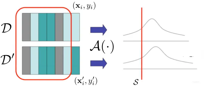
, (where the likelihood is over the randomness in the algorithm). That is, any single entry of the data set does not affect the output distribution of the algorithm by much; dually, this means that an adversary, who knows all but one entry of the data set, cannot gain much additional information about the last entry by observing the output of the algorithm.D
D
′
(
x
i, y
i)
(
x
′i
, y
i′)
A
(
·
)
S
Figure 1: An algorithm which is differentially private. When data sets which are identical except for a single entry are input to the algorithm
A
, the two distributions on the algorithm’s output are close. For a fixed measurableS
the ratio of the measures (or densities) should be bounded.Definition 2 An algorithm
A
(B
)taking values in a setT
providesεp-differential privacy ifsup S
sup D,D′
µ(
S
|B
=D
) µ(S
|B
=D
′)≤eεp, (2)
where the first supremum is over all measurable
S
⊆T
, the second is over all data setsD
andD
′differing in a single entry, and µ(·|
B
) is the conditional distribution (measure) onT
induced by the outputA
(B
)given a data setB
. The ratio is interpreted to be 1 whenever the numerator and denominator are both 0.Note that if
S
is a set of measure 0 under the conditional measures induced byD
andD
′, the ratio is automatically 1. A more measure-theoretic definition is given in Zhou et al. (2009). An illustration of the definition is given in Figure 1.The following form of the definition is due to Dwork et al. (2006a).
Definition 3 An algorithm
A
providesεp-differential privacy if for any two data setsD
andD
′thatdiffer in a single entry and for any set
S
,exp(−εp)P(
A
(D
′)∈S
)≤P(A
(D
)∈S
)≤exp(εp)P(A
(D
′)∈S
), (3)where
A
(D
)(resp.A
(D
′)) is the output ofA
on inputD
(resp.D
′).We observe that an algorithm
A
that satisfies Equation 2 also satisfies Equation 3, and as a result, Definition 2 is stronger than Definition 3.From this definition, it is clear that the
A
(D
)that outputs the minimizer of the ERM objective (1) does not provideεp-differential privacy for anyεp. This is because an ERM solution is a linearinfinite. Regularization helps by penalizing the L2 norm of the change, but does not account how
the direction of the minimizer is sensitive to changes in the data.
Dwork et al. (2006b) also provide a standard recipe for computing privacy-preserving approxi-mations to functions by adding noise with a particular distribution to the output of the function. We call this recipe the sensitivity method. Let g :(Rm)n→Rbe a scalar function of z
1, . . . ,zn, where
zi∈Rmcorresponds to the private value of individual i; then the sensitivity of g is defined as follows.
Definition 4 The sensitivity of a function g :(Rm)n→Ris maximum difference between the values
of the function when one input changes. More formally, the sensitivity S(g)of g is defined as:
S(g) =max
i z1max,...,zn,z′i
g(z1, . . . ,zi−1,zi,zi+1, . . . ,zn)−g(z1, . . . ,zi−1,zi′,zi+1, . . . ,zn) .
To compute a function g on a data set
D
={z1, . . . ,zn}, the sensitivity method outputsg(z1, . . . ,zn) +η, whereηis a random variable drawn according to the Laplace distribution, with
mean 0 and standard deviation Sε(g)
p . It is shown in Dwork et al. (2006b) that such a procedure is
εp-differentially private.
3. Privacy-preserving ERM
Here we describe two approaches for creating privacy-preserving algorithms from (1).
3.1 Output Perturbation: The Sensitivity Method
Algorithm 1 is derived from the sensitivity method of Dwork et al. (2006b), a general method for generating a privacy-preserving approximation to any function A(·). In this section the normk · k is the L2-norm unless otherwise specified. For the function A(
D
) =argmin J(f,D
), Algorithm 1outputs a vector A(
D
) +b, where b is random noise with densityν(b) = 1
αe−βkbk, (4)
whereα is a normalizing constant. The parameterβ is a function ofεp, and the L2-sensitivity of
A(·), which is defined as follows.
Definition 5 The L2-sensitivity of a vector-valued function is defined as the maximum change in the L2norm of the value of the function when one input changes. More formally,
S(A) =max
i z1max,...,zn,z′i
A(z1, . . . ,zi, . . .)−A(z1, . . . ,z′i, . . .)
.
Algorithm 1 ERM with output perturbation (sensitivity) Inputs: Data
D
={zi}, parametersεp,Λ.Output: Approximate minimizer fpriv.
Draw a vector b according to (4) withβ=nΛεp
2 .
Compute fpriv=argmin J(f,
D
) +b.3.2 Objective Perturbation
A different approach, first proposed by Chaudhuri and Monteleoni (2008), is to add noise to the objective function itself and then produce the minimizer of the perturbed objective. That is, we can minimize
Jpriv(f,
D
) =J(f,D
) +1
nb
Tf,
where b has density given by (4), withβ=εp. Note that the privacy parameter here does not depend
on the sensitivity of the of the classification algorithm.
Algorithm 2 ERM with objective perturbation Inputs: Data
D
={zi}, parametersεp,Λ, c. Output: Approximate minimizer fpriv.Letε′p=εp−log(1+n2cΛ+ c
2
n2Λ2).
Ifε′p>0, then∆=0, else∆= c
n(eεp/4−1)−Λ, andε′p=εp/2.
Draw a vector b according to (4) withβ=ε′p/2. Compute fpriv=argmin Jpriv(f,
D
) +12∆||f||2.The algorithm requires a certain slack, log(1+2c nΛ+
c2
n2Λ2), in the privacy parameter. This is due
to additional factors in bounding the ratio of the densities. The “If” statement in the algorithm is from having to consider two cases in the proof of Theorem 9, which shows that the algorithm is differentially private.
3.3 Privacy Guarantees
In this section, we establish the conditions under which Algorithms 1 and 2 provideεp-differential
privacy. First, we establish guarantees for Algorithm 1.
3.3.1 PRIVACYGUARANTEES FOROUTPUTPERTURBATION
Theorem 6 If N(·)is differentiable, and 1-strongly convex, andℓis convex and differentiable, with
|ℓ′(z)| ≤1 for all z, then, Algorithm 1 providesεp-differential privacy.
The proof of Theorem 6 follows from Corollary 8, and Dwork et al. (2006b). The proof is provided here for completeness.
Proof From Corollary 8, if the conditions on N(·)andℓhold, then the L2-sensivity of ERM with
regularization parameterΛis at most n2Λ. We observe that when we pick||b||from the distribution in Algorithm 1, for a specific vector b0∈Rd, the density at b0is proportional to e−
nΛεp
and
D
′be any two data sets that differ in the value of one individual. Then, for any f,g(f|
D
) g(f|D
′) =ν(b1) ν(b2) =e
−nΛε2p(||b1||−||b2||),
where b1and b2are the corresponding noise vectors chosen in Step 1 of Algorithm 1, and g(f|
D
)(g(f|
D
′) respectively) is the density of the output of Algorithm 1 at f, when the input isD
(D
′ respectively). If f1 and f2are the solutions respectively to non-private regularized ERM when theinput is
D
andD
′, then, b2−b1=f2−f1. From Corollary 8, and using a triangle inequality,||b1|| − ||b2|| ≤ ||b1−b2||=||f2−f1|| ≤ 2
nΛ.
Moreover, by symmetry, the density of the directions of b1and b2are uniform. Therefore, by
con-struction, ν(b1) ν(b2)≤e
εp. The theorem follows.
The main ingredient of the proof of Theorem 6 is a result about the sensitivity of regularized ERM, which is provided below.
Lemma 7 Let G(f)and g(f) be two vector-valued functions, which are continuous, and differen-tiable at all points. Moreover, let G(f) and G(f) +g(f)beλ-strongly convex. If f1=argminfG(f)
and f2=argminfG(f) +g(f), then
kf1−f2k ≤ 1
λmaxf k∇g(f)k.
Proof Using the definition of f1and f2, and the fact that G and g are continuous and differentiable
everywhere,
∇G(f1) =∇G(f2) +∇g(f2) =0. (5) As G(f)isλ-strongly convex, it follows from Lemma 14 of Shalev-Shwartz (2007) that:
(∇G(f1)−∇G(f2))T(f1−f2)≥λkf1−f2k2.
Combining this with (5) and the Cauchy-Schwartz inequality, we get that
kf1−f2k · k∇g(f2)k ≥(f1−f2)T∇g(f2) = (∇G(f1)−∇G(f2))T(f1−f2)≥λkf1−f2k2.
The conclusion follows from dividing both sides byλkf1−f2k.
Corollary 8 If N(·)is differentiable and 1-strongly convex, andℓis convex and differentiable with
|ℓ′(z)| ≤1 for all z, then, the L2-sensitivity of J(f,
D
)is at most n2Λ.Proof Let
D
={(x1,y1), . . . ,(xn,yn)}andD
′={(x1,y1), . . . ,(x′n,y′n)}be two data sets that differin the value of the n-th individual. Moreover, we let G(f) =J(f,
D
), g(f) =J(f,D
′)−J(f,D
),We observe that due to the convexity of ℓ, and 1-strong convexity of N(·), G(f) =J(f,
D
) isΛ-strongly convex. Moreover, G(f) +g(f) =J(f,
D
′)is alsoΛ-strongly convex. Finally, due to the differentiability of N(·)andℓ, G(f)and g(f)are also differentiable at all points. We have:∇g(f) =1 n(ynℓ
′(y
nfTxn)xn−y′nℓ′(y′nfTx′n)x′n).
As yi∈[−1,1],|ℓ′(z)| ≤1, for all z, and||xi|| ≤1, for any f,||∇g(f)|| ≤ 1n(||xn−xn′||)≤1n(||xn||+
||x′n||)≤2
n. The proof now follows by an application of Lemma 7.
3.3.2 PRIVACYGUARANTEES FOROBJECTIVEPERTURBATION
In this section, we show that Algorithm 2 isεp-differentially private. This proof requires stronger
assumptions on the loss function than were required in Theorem 6. In certain cases, some of these assumptions can be weakened; for such an example, see Section 3.4.2.
Theorem 9 If N(·) is 1-strongly convex and doubly differentiable, andℓ(·) is convex and doubly differentiable, with|ℓ′(z)| ≤1 and|ℓ′′(z)| ≤c for all z, then Algorithm 2 isεp-differentially private.
Proof Consider an fpriv output by Algorithm 2. We observe that given any fixed fpriv and a fixed
data set
D
, there always exists a b such that Algorithm 2 outputs fpriv on inputD
. Because ℓis differentiable and convex, and N(·) is differentiable, we can take the gradient of the objective function and set it to 0 at fpriv. Therefore,
b=−nΛ∇N(fpriv)− n
∑
i=1
yiℓ′(yifTprivxi)xi−n∆fpriv. (6)
Note that (6) holds because for any f,∇ℓ(fTx) =ℓ′(fTx)x.
We claim that as ℓis differentiable and J(f,
D
) +∆2||f||2 is strongly convex, given a data setD
= (x1,y1), . . . ,(xn,yn), there is a bijection between b and fpriv. The relation (6) shows that twodifferent b values cannot result in the same fpriv. Furthermore, since the objective is strictly convex,
for a fixed b and
D
, there is a unique fpriv; therefore the map from b to fprivis injective. The relation(6) also shows that for any fpriv there exists a b for which fprivis the minimizer, so the map from b
to fprivis surjective.
To showεp-differential privacy, we need to compute the ratio g(fpriv|
D
)/g(fpriv|D
′)of theden-sities of fprivunder the two data sets
D
andD
′. This ratio can be written as (Billingsley, 1995)g(fpriv|
D
)g(fpriv|
D
′) =µ(b|
D
) µ(b′|D
′)·|det(J(fpriv→b|
D
))|−1|det(J(fpriv→b′|
D
′))|−1,where J(fpriv→b|
D
), J(fpriv→b|D
′) are the Jacobian matrices of the mappings from fpriv to b,and µ(b|
D
)and µ(b|D
′)are the densities of b given the output fpriv, when the data sets areD
andD
′respectively.First, we bound the ratio of the Jacobian determinants. Let b(j)denote the j-th coordinate of b. From (6) we have
b(j)=−nΛ∇N(fpriv)(j)−
n
∑
i=1
ℓ′(yifTprivxi)x(ij)−n∆f
(j)
Given a data set
D
, the(j,k)-th entry of the Jacobian matrix J(f→b|D
)is∂b(j)
∂f(k)
priv
=−nΛ∇2N(fpriv)(j,k)−
∑
i
y2iℓ′′(yifprivT xi)xi(j)x(ik)−n∆1(j=k),
where 1(·)is the indicator function. We note that the Jacobian is defined for all fprivbecause N(·)
andℓare globally doubly differentiable.
Let
D
andD
′be two data sets which differ in the value of the n-th item such thatD
={(x1,y1), . . . ,(xn−1,yn−1),(xn,yn)} andD
′={(x1,y1), . . . ,(xn−1,yn−1),(x′n,y′n)}. Moreover,we define matrices A and E as follows:
A=nΛ∇2N(fpriv) +
n
∑
i=1
y2iℓ′′(yifTprivxi)xixTi +n∆Id,
E=−y2nℓ′′(ynfTprivxn)xnxTn + (yn′)2ℓ′′(y′nfTprivx′n)x′nx′Tn.
Then, J(fpriv→b|
D
) =−A, and J(fpriv→b|D
′) =−(A+E).Letλ1(M)andλ2(M) denote the largest and second largest eigenvalues of a matrix M. As E has rank at most 2, from Lemma 10,
|det(J(fpriv→b|
D
′))||det(J(fpriv→b|
D
))| =|det(A+E)|
|det A|
=|1+λ1(A−1E) +λ2(A−1E) +λ1(A−1E)λ2(A−1E)|.
For a 1-strongly convex function N, the Hessian∇2N(f
priv)has eigenvalues greater than 1 (Boyd and
Vandenberghe, 2004). Since we have assumedℓis doubly differentiable and convex, any eigenvalue of A is therefore at least nΛ+n∆; therefore, for j=1,2,|λj(A−1E)| ≤ n|λ(Λ+∆)j(E)|. Applying the triangle
inequality to the trace norm:
|λ1(E)|+|λ2(E)| ≤ |yn2ℓ′′(ynfTprivxn)| · kxnk+| −(y′n)2ℓ′′(y′nfTprivx′n)| ·
x′n
.
Then upper bounds on|yi|,||xi||, and|ℓ′′(z)|yield
|λ1(E)|+|λ2(E)| ≤2c.
Therefore,|λ1(E)| · |λ2(E)| ≤c2, and
|det(A+E)|
|det(A)| ≤1+
2c
n(Λ+∆)+ c2 n2(Λ+∆)2 =
1+ c
n(Λ+∆)
2
.
We now consider two cases. In the first case,∆=0, and by definition, in that case, 1+2c nΛ+
c2 n2Λ2 ≤ eεp−ε′p. In the second case,∆>0, and in this case, by definition of∆,(1+ c
n(Λ+∆))
2=eεp/2=eεp−ε′p.
Next, we bound the ratio of the densities of b. We observe that as |ℓ′(z)| ≤1, for any z and
|yi|,||xi|| ≤1, for data sets
D
andD
′which differ by one value,This implies that:
kbk −b′
≤
b−b′
≤2.
We can write:
µ(b|
D
) µ(b′|D
′)=||b||d−1e−ε′p||b||/2· 1
surf(||b||)
||b′||d−1e−ε′p||b′||/2· 1
surf(||b′||)
≤eε′p(||b||−||b′||)/2≤eε′p,
where surf(x) denotes the surface area of the sphere in d dimensions with radius x. Here the last step follows from the fact that surf(x) =surf(1)xd−1, where surf(1)is the surface area of the unit
sphere inRd.
Finally, we are ready to bound the ratio of densities:
g(fpriv|
D
)g(fpriv|
D
′) =µ(b|
D
) µ(b′|D
′)·|det(J(fpriv→b|
D
′))||det(J(fpriv→b′|
D
))|= µ(b|
D
)µ(b′|
D
′)·|det(A+E)|
|det A|
≤eε′p·eεp−ε′p ≤eεp.
Thus, Algorithm 2 satisfies Definition 2.
Lemma 10 If A is full rank, and if E has rank at most 2, then,
det(A+E)−det(A)
det(A) =λ1(A
−1E) +λ2(A−1E) +λ1(A−1E)λ2(A−1E),
whereλj(Z)is the j-th eigenvalue of matrix Z.
Proof Note that E has rank at most 2, so A−1E also has rank at most 2. Using the fact that
λi(I+A−1E) =1+λi(A−1E),
det(A+E)−det(A)
det A =det(I+A
−1E)−1
= (1+λ1(A−1E))(1+λ2(A−1E))−1
=λ1(A−1E) +λ2(A−1E) +λ1(A−1E)λ2(A−1E).
3.4 Application to Classification
3.4.1 LOGISTIC REGRESSION
One popular ERM classification algorithm is regularized logistic regression. In this case, N(f) =
1 2||f||
2, and the loss function isℓ
LR(z) =log(1+e−z). Taking derivatives and double derivatives,
ℓ′LR(z) = −1
(1+ez),
ℓ′′LR(z) = 1
(1+e−z)(1+ez).
Note thatℓLRis continuous, differentiable and doubly differentiable, with c≤14. Therefore, we can
plug in logistic loss directly to Theorems 6 and 9 to get the following result.
Corollary 11 The output of Algorithm 1 with N(f) = 1
2||f||2,ℓ=ℓLRis anεp-differentially private
approximation to logistic regression. The output of Algorithm 2 with N(f) = 12||f||2, c= 14, and
ℓ=ℓLR, is anεp-differentially private approximation to logistic regression.
We quantify how well the outputs of Algorithms 1 and 2 approximate (non-private) logistic regression in Section 4.
3.4.2 SUPPORT VECTORMACHINES
Another very commonly used classifier is L2-regularized support vector machines. In this case,
again, N(f) =1 2||f||
2, and
ℓSVM(z) =max(0,1−z).
Notice that this loss function is continuous, but not differentiable, and thus it does not satisfy con-ditions in Theorems 6 and 9.
There are two alternative solutions to this. First, we can approximateℓSVMby a different loss
function, which is doubly differentiable, as follows (see also Chapelle, 2007):
ℓs(z) =
0 if z>1+h
−(116h−z3)4+
3(1−z)2
8h + 1−z
2 + 3h
16 if |1−z| ≤h
1−z if z<1−h.
As h→0, this loss approaches the hinge loss. Taking derivatives, we observe that:
ℓ′s(z) =
0 if z>1+h
(1−z)3
4h3 −
3(1−z)
4h − 1
2 if |1−z| ≤h
−1 if z<1−h.
Moreover,
ℓ′′s(z) =
0 if z>1+h
−3(14h−3z)2 +4h3 if |1−z| ≤h
0 if z<1−h.
Observe that this implies that|ℓ′′
s(z)| ≤ 4h3 for all h and z. Moreover,ℓsis convex, asℓ′′s(z)≥0 for all
z. Therefore,ℓscan be used in Theorems 6 and 9, which gives us privacy-preserving approximations
Corollary 12 The output of Algorithm 1 with N(f) =1
2||f||2, andℓ=ℓsis anεp-differentially private
approximation to support vector machines. The output of Algorithm 2 with N(f) =12||f||2, c=4h3, andℓ=ℓsis anεp-differentially private approximation to support vector machines.
The second solution is to use Huber Loss, as suggested by Chapelle (2007), which is defined as follows:
ℓHuber(z) =
0 if z>1+h
1
4h(1+h−z)
2 if |1−z| ≤h
1−z if z<1−h.
(7)
Observe that Huber loss is convex and differentiable, and piecewise doubly-differentiable, with
c= 1
2h. However, it is not globally doubly differentiable, and hence the Jacobian in the proof of
Theorem 9 is undefined for certain values of f. However, we can show that in this case, Algorithm 2, when run with c= 1
2h satisfies Definition 3.
Let G denote the map from fprivto b in (6) under
B
=D
, and H denote the map underB
=D
′.By definition, the probabilityP(fpriv∈
S
|B
=D
) =Pb(b∈G(S
)).Corollary 13 Let fprivbe the output of Algorithm 2 withℓ=ℓHuber, c=2h1, and N(f) = 12||f||22. For
any set
S
of possible values of fpriv, and any pair of data setsD
,D
′which differ in the private valueof one person(xn,yn),
e−εpP(
S
|B
=D
′)≤P(S
|B
=D
)≤eεpP(S
|B
=D
′).Proof Consider the event fpriv∈
S
. LetT
=G(S
)andT
′=H(S
). Because G is a bijection, we haveP(fpriv∈
S
|B
=D
) =Pb(b∈T
|B
=D
),and a similar expression when
B
=D
′. Now note thatℓ′Huber(z) is only non-differentiable for a finite number of values of z. Let
Z
bethe set of these values of z.
C
={f : yfTx=z∈Z
, (x,y)∈D
∪D
′}.Pick a tuple (z,(x,y))∈
Z
×(D
∪D
′). The set of f such that yfTx=z is a hyperplane in Rd.Since∇N(f) =f/2 andℓ′ is piecewise linear, from(6)we see that the set of corresponding b’s is also piecewise linear, and hence has Lebesgue measure 0. Since the measure corresponding to b is absolutely continuous with respect to the Lebesgue measure, this hyperplane has probability 0 under b as well. Since
C
is a finite union of such hyperplanes, we haveP(b∈G(C
)) =0.Thus we havePb(
T
|B
=D
) =Pb(G(S
\C
)|B
=D
), and similarly forD
′. From the definitionof G and H, for f∈
S
\C
,H(f) =G(f) +ynℓ′(ynfTxn)xn−y′nℓ′(y′nfTx′n)x′n.
since f∈/
C
, this mapping shows that if Pb(G(S
\C
)|B
=D
) =0 then we must have Pb(H(S
\calculate the ratio of the probabilities for fpriv for which the loss is twice-differentiable. For such fprivthe Jacobian is also defined, and we can use a method similar to Theorem 9 to prove the result.
Remark: Because the privacy proof for Algorithm 1 does not require the analytic properties of
2, we can also use Huber loss in Algorithm 1 to get anεg-differentially private approximation to the
SVM. We quantify how well the outputs of Algorithms 1 and 2 approximate private support vector machines in Section 4. These approximations to the hinge loss are necessary because of the analytic requirements of Theorems 6 and 9 on the loss function. Because the requirements of Theorem 9 are stricter, it may be possible to use an approximate loss in Algorithm 1 that would not be admissible in Algorithm 2.
4. Generalization Performance
In this section, we provide guarantees on the performance of privacy-preserving ERM algorithms in Section 3. We provide these bounds for L2-regularization. To quantify this performance, we will
assume that the n entries in the data set
D
are drawn i.i.d. according to a fixed distribution P(x,y). We measure the performance of these algorithms by the number of samples n required to acheive error L∗+εg, where L∗is the loss of a reference ERM predictor f0. This resulting bound onεgwilldepend on the normkf0k of this predictor. By choosing an upper boundν on the norm, we can interpret the result as saying that the privacy-preserving classifier will have errorεgmore than that
of any predictor withkf0k ≤ν.
Given a distribution P the expected loss L(f)for a classifier f is
L(f) =E(x,y)∼P
ℓ(fTx,y)
.
The sample complexity for generalization error εg against a classifier f0 is number of samples n
required to achieve error L(f0) +εg under any data distribution P. We would like the sample
com-plexity to be low.
For a fixed P we define the following function, which will be useful in our analysis:
¯
J(f) =L(f) +Λ
2kfk
2 .
The function ¯J(f)is the expectation (over P) of the non-private L2-regularized ERM objective
eval-uated at f.
For non-private ERM, Shalev-Shwartz and Srebro (2008) show that for a given f0 with loss
L(f0) =L∗, if the number of data points satisfies
n>C||f0||
2log(1
δ)
ε2 g
for some constant C, then the excess loss of the L2-regularized SVM solution fsvmsatisfies L(fsvm)≤
L(f0) +εg. This order growth will hold for our results as well. It also serves as a reference against
which we can compare the additional burden on the sample complexity imposed by the privacy constraints.
For most learning problems, we require the generalization errorεg<1. Moreover, it is also
SVM, ||f1
0|| is the margin of classification, and as a result,||f0||is higher for learning problems with
smaller margin. From the bounds provided in this section, we note that the dominating term in the sample requirement for objective perturbation has a better dependence on||f0||as well as ε1g; as a
result, for more difficult learning problems, we expect objective perturbation to perform better than output perturbation.
4.1 Output Perturbation
First, we provide performance guarantees for Algorithm 1, by providing a bound on the number of samples required for Algorithm 1 to produce a classifier with low error.
Definition 14 A function g(z):R→Ris c-Lipschitz if for all pairs(z1,z2)we have|g(z1)−g(z2)| ≤
c|z1−z2|.
Recall that if a function g(z) is differentiable, with|g′(z)| ≤r for all z, then g(z) is also r-Lipschitz.
Theorem 15 Let N(f) =1 2||f||
2, and let f
0be a classifier such that L(f0) =L∗, and letδ>0. Ifℓis
differentiable and continuous with|ℓ′(z)| ≤1, the derivativeℓ′ is c-Lipschitz, the data
D
is drawn i.i.d. according to P, then there exists a constant C such that if the number of training samples satisfiesn>C max ||f0||
2log(1
δ)
ε2 g
,d log( d
δ)||f0|| εgεp
,d log( d
δ)c1/2||f0||2 ε3/2
g εp
!
, (8)
where d is the dimension of the data space, then the output fprivof Algorithm 1 satisfies P L(fpriv)≤L∗+εg
≥1−2δ.
Proof Let
frtr=argmin
f
¯
J(f), f∗=argmin
f
J(f,
D
),and fprivdenote the output of Algorithm 1. Using the analysis method of Shalev-Shwartz and Srebro
(2008) shows
L(fpriv) =L(f0) + (J(¯fpriv)−J(¯frtr)) + (J(¯frtr)−J(¯f0)) +
Λ
2||f0||
2
−Λ2||fpriv||2. (9)
We will bound the terms on the right-hand side of (9). For a regularizer N(f) = 1
2||f||2the Hessian satisfies||∇2N(f)||2≤1 . Therefore, from Lemma
16, with probability 1−δover the privacy mechanism,
J(fpriv,
D
)−J(f∗,D
)≤8d2log2(d/δ)(c+Λ)
Λ2n2ε2 p
Furthermore, the results of Sridharan et al. (2008) show that with probability 1−δover the choice of the data distribution,
¯
J(fpriv)−J(¯frtr)≤2(J(fpriv,
D
)−J(f∗,D
)) +O
log(1/δ)
Λn
.
The constant in the last term depends on the derivative of the loss and the bound on the data points, which by assumption are bounded. Combining the preceeding two statements, with probability 1−2δover the noise in the privacy mechanism and the data distribution, the second term in the right-hand-side of (9) is at most:
¯
J(fpriv)−J(¯frtr)≤
16d2log2(d/δ)(c+Λ)
Λ2n2ε2 p
+O
log(1/δ)
Λn
. (10)
By definition of frtr, the difference(J(¯frtr)−J(¯f0))≤0. SettingΛ= ||fεg
0||2 in (9) and using (10), we
obtain
L(fpriv)≤L(f0) +16||f0||
4d2log2(d/δ)(c+ε
g/||f0||2)
n2ε2 gε2p
+O
||f0||2log(1/δ)
nεg
+εg
2.
Solving for n to make the total excess error equal toεgyields (8).
Lemma 16 Suppose N(·)is doubly differentiable with||∇2N(f)||2≤ηfor all f, and suppose thatℓ
is differentiable and has continuous and c-Lipschitz derivatives. Given training data
D
, let f∗be a classifier that minimizes J(f,D
)and let fprivbe the classifier output by Algorithm 1. ThenPb J(fpriv,
D
)≤J(f∗,D
) +2d2(c+Λη)log2(d/δ)
Λ2n2ε2 p
!
≥1−δ,
where the probability is taken over the randomness in the noise b of Algorithm 1.
Note that whenℓis doubly differentiable, c is an upper bound on the double derivative ofℓ, and is the same as the constant c in Theorem 9.
Proof Let
D
={(x1,y1), . . . ,(xn,yn)}, and recall that ||xi|| ≤1, and|yi| ≤1. As N(·) andℓaredifferentiable, we use the Mean Value Theorem to show that for some t between 0 and 1,
J(fpriv,
D
)−J(f∗,D
) = (fpriv−f∗)T∇J(tf∗+ (1−t)fpriv)≤ ||fpriv−f∗|| · ||∇J(tf∗+ (1−t)fpriv)||, (11) where the second step follows by an application of the Cauchy-Schwartz inequality. Recall that
∇J(f,
D
) =Λ∇N(f) +1 n∑
i yiℓ′(y
ifTxi)xi.
Moreover, recall that∇J(f∗,
D
) =0, from the optimality of f∗. Therefore,∇J(tf∗+ (1−t)fpriv,
D
) =∇J(f∗,D
)−Λ(∇N(f∗)−∇N(tf∗+ (1−t)fpriv))−1n
∑
i
yi ℓ′(yi(f∗)Txi)−ℓ′(yi(tf∗+ (1−t)fpriv)Txi)
Now, from the Lipschitz condition onℓ, for each i we can upper bound each term in the summation above:
yi ℓ′(yi(f∗)Txi)−ℓ′(yi(tf∗+ (1−t)fpriv)Txi)
xi
≤ |yi| · ||xi|| · |ℓ′(yi(f∗)Txi)−ℓ′(yi(tf∗+ (1−t)fpriv)Txi)|
≤ |yi| · ||xi|| ·c· |yi(1−t)(f∗−fpriv)Txi|
≤c(1−t)|yi|2· ||xi||2· ||f∗−fpriv||
≤c(1−t)||f∗−fpriv||. (13)
The third step follows becauseℓ′is c-Lipschitz and the last step follows from the bounds on|yi|and
||xi||. Because N is doubly differentiable, we can apply the Mean Value Theorem again to conclude
that
||∇N(tf∗+ (1−t)fpriv)−∇N(f∗)|| ≤(1−t)||fpriv−f∗|| · ||∇2N(f′′)||2 (14)
for some f′′∈Rd.
As 0≤t≤1, we can combine (12), (13), and (14) to obtain
∇J(tf∗+ (1−t)fpriv,
D
)≤
Λ(∇N(f∗)−∇N(tf∗+ (1−t)fpriv))
+
1
n
∑
i yi(ℓ ′(yi(f∗)Txi)−ℓ′(yi(tf∗+ (1−t)fpriv)Txi))xi
≤(1−t)fpriv−f∗
·
Λη+1 n·n·c
≤
fpriv−f∗
(Λη+c). (15)
From the definition of Algorithm 1, fpriv−f∗=b, where b is the noise vector. Now we can apply
Lemma 17 to||fpriv−f∗||, with parameters k=d, andθ=Λn2εp. From Lemma 17, with probability
1−δ,||fpriv−f∗|| ≤ 2d log(dδ)
Λnεp . The Lemma follows by combining this with Equations 15 and 11.
Lemma 17 Let X be a random variable drawn from the distributionΓ(k,θ), where k is an integer. Then,
P
X<kθlog
k
δ
≥1−δ.
Proof Since k is an integer, we can decompose X distributed according toΓ(k,θ)as a summation
where X1,X2, . . . ,Xkare independent exponential random variables with meanθ. For each i we have
P(Xi≥θlog(k/δ)) =δ/k. Now,
P(X<kθlog(k/δ))≥P(Xi<θlog(k/δ)i=1,2, . . . ,k)
= (1−δ/k)k
≥1−δ.
4.2 Objective Perturbation
We now establish performance bounds on Algorithm 2. The bound can be summarized as follows.
Theorem 18 Let N(f) = 1 2||f||
2, and let f
0 be a classifier with expected loss L(f0) =L∗. Let ℓbe
convex, doubly differentiable, and let its derivatives satisfy|ℓ′(z)| ≤1 and|ℓ′′(z)| ≤c for all z. Then there exists a constant C such that forδ>0, if the n training samples in
D
are drawn i.i.d. according to P, and ifn>C max ||f0||
2log(1/δ) ε2
g
,c||f0|| 2 εgεp
,d log( d
δ)||f0|| εgεp
!
,
then the output fprivof Algorithm 2 satisfies
P L(fpriv)≤L∗+εg
≥1−2δ.
Proof Let
frtr=argmin
f
¯
J(f), f∗=argmin
f
J(f,
D
),and fprivdenote the output of Algorithm 1. As in Theorem 15, the analysis of Shalev-Shwartz and
Srebro (2008) shows
L(fpriv) =L(f0) + (J(¯fpriv)−J(¯frtr)) + (J(¯frtr)−J(¯f0)) +
Λ
2||f0||
2−Λ
2||fpriv||
2. (16)
We will bound each of the terms on the right-hand-side. If n>c||f0||2
εgεp andΛ>
εg
4||f0||2, then nΛ>
c
4εp, so from the definition ofε
′
pin Algorithm 2,
ε′
p=εp−2 log
1+ c
nΛ
=εp−2 log
1+εp
4
≥εp−
εp
2,
Therefore, we can apply Lemma 19 to conclude that with probability at least 1−δ over the privacy mechanism,
J(fpriv,
D
)−J(f∗,D
)≤4d2log2(d/δ)
Λn2ε2 p
.
From Sridharan et al. (2008),
¯
J(fpriv)−J(¯frtr)≤2(J(fpriv,
D
)−J(f∗,D
)) +O
log(1/δ)
Λn
≤8d
2log2(d/δ) Λn2ε2
p
+O
log(1/δ)
Λn
.
By definition of f∗, we have ¯J(frtr)−J(¯f0)≤0. IfΛis set to be ||fεg
0||2, then, the fourth quantity
in Equation 16 is at most εg
2. The theorem follows by solving for n to make the total excess error at
mostεg.
The following lemma is analogous to Lemma 16, and it establishes a bound on the distance between the output of Algorithm 2, and non-private regularized ERM. We note that this bound holds when Algorithm 2 hasε′p>0, that is, when∆=0. Ensuring that∆=0 requires an additional condition on n, which is stated in Theorem 18.
Lemma 19 Letε′p>0. Let f∗=argmin J(f,
D
), and let fpriv be the classifier output by Algorithm2. If N(·)is 1-strongly convex and globally differentiable, and ifℓis convex and differentiable at all points, with|ℓ′(z)| ≤1 for all z, then
Pb J(fpriv,
D
)≤J(f∗,D
) +4d2log2(d/δ)
Λn2ε2 p
!
≥1−δ,
where the probability is taken over the randomness in the noise b of Algorithm 2.
Proof By the assumptionε′p>0, the classifier fprivminimizes the objective function J(f,
D
) +1nbTf,and therefore
J(fpriv,
D
)≤J(f∗,D
) +1
nb
T(f∗
−fpriv).
First, we try to bound ||f∗−fpriv||. Recall that ΛN(·)isΛ-strongly convex and globally differen-tiable, andℓis convex and differentiable. We can therefore apply Lemma 7 with G(f) =J(f,
D
)andg(f) =1
nbTf to obtain the bound
||f∗−fpriv|| ≤
1
Λ
∇
(1
nb
Tf)
≤
||b||
nΛ .
Therefore by the Cauchy-Schwartz inequality,
J(fpriv,
D
)−J(f∗,D
)≤||b||2
n2Λ .
Since ||b||is drawn from aΓ(d,2
εp)distribution, from Lemma 17, with probability 1−δ, ||b|| ≤
2d log(d/δ)