Solving multi-order fractional differential equations by reproducing kernel Hilbert space method

(1)

Solving multi-order fractional diﬀerential equations by reproducing

kernel Hilbert space method

R. Khoshsiar Ghaziani∗

Department of Applied Mathematics, Faculty of Mathematical Science, Shahrekord University, Shahrekord, P. O. Box 115, Iran.

E-mail: [email protected]

M. Fardi

E-mail: fardi [email protected]

M. Ghasemi

E-mail: meh [email protected]

Abstract In this paper, we propose a relatively new semi-analytical technique to approximate the solution of nonlinear multi-order fractional diﬀerential equations (FDEs). We present some results concerning to the uniqueness of solution of nonlinear multi-order FDEs and discuss the existence of solution for nonlinear multi-multi-order FDEs in reproducing kernel Hilbert space (RKHS). We further give an error analysis for the proposed technique in diﬀerent reproducing kernel Hilbert spaces and present some useful results. The accuracy of the proposed technique is examined by comparing with the exact solution of some test examples.

Keywords. Multi-Order Fractional; Hilbert space; Reproducing kernel method; Uniqueness; Existence; Error analysis.

2010 Mathematics Subject Classification. 34A08.

1. Introduction

Fractional differential equations have gained considerable importance due to their frequent applications in various fields of science and engineering [1-2], integral equa-tions [3], viscoelastic damping materials [4-5], bioengineering [6-8], solid mechanics [9], chaos [10-11], control theory [12] and finance [13-14]. It has been found that frac-tional derivatives provide an excellent instrument for the description of memory and hereditary properties of different substances. Due to these features, the fractional-order models become more practical and realistic than the classical integrad-fractional-order models, in which such effects are not taken into account. Finding exact solutions in closed forms for most differential equations of fractional order is a difficult task

Received: 11 October 2016 ; Accepted: 18 December 2016. ∗Corresponding author.

(2)

[15-16]. As a result, a number of methods have been proposed and applied success-fully to approximate fractional differential equations, such as Adomian decomposition method [17], variational iteration method [18], homotopy analysis method [19] and collocation method [20]. Especially, Momani and Odibat [21-22], have applied He’s variational iteration method to fractional differential equations. Meanwhile, vari-ous fractional order differential equation have been solved very recently including fractional advection-dispersion equations [23-24], reaction-diffusion system with frac-tional derivatives [25], fracfrac-tional partial differential equations fluid mechanics [26] and fractional-order multi-point boundary value problem [27-29]. Fractional differential equations with multi-orders have been used to model different types [30-33].

In the present work, we are concerned with the numerical solution of the following multi-order fractional diﬀerential equations in a reproducing kernel space method (RKSM):

Dαn

∗τϕ(τ) = f(τ, ϕ(τ),D_∗ατ1ϕ(τ),D_∗ατ2ϕ(τ),· · ·,D αn−1

∗τ ϕ(τ)), (1.1)

D(j)ϕ(0) = 0, j= 0,1,2,· · · , n−1 n∈ N,

where 0 ≤ α1 < α2 < · · · < αn₋1 < αn ≤ n and f is a given function on

D := [0, T]×Rn _and _Dαi

∗τ stands for the Caputo fractional derivative of order αi.

Recently, the(RKSM) [34-35], has been used for obtaining approximate solutions of differential and integral equations [36-45]. However, due to the multi-point initial value conditions in (1), especially for fractional differential equations, it is difficult to find the corresponding reproducing kernel space by applying traditional RKSM. The aim of this work is to extend the RKSM to derive the numerical solutions of (1). One important improvement is that we successfully construct a novel reproducing kernel space to overcome difficulties with the multi order FDEs. By using the new repro-ducing kernel functions, we present an efficient numerical algorithm to solve (1). We especially emphasis on the uniformly convergence of the approximate solution and error estimation of our algorithm are studied.

The rest of paper is organized as follows. In Section 2, we present some important deﬁnitions and preparations used in this paper. In Section 3, we construct and de-velop algorithms for solving nonlinear fractional diﬀerential equation. In Section 4 the proposed methods are applied to several examples. Also a conclusion is given in Section 5.

2. _{Fractional Calculus}

We now give some basic definitions and properties of the fractional calculus theory, which are used in the following sections. For more details see [15-16]. For the finite derivative in [0, T], we define the following fractional integral and derivatives.

Deﬁnition 2.1. (see [15-16]). A real functionϕ(τ), τ >0,is said to be in the space

Cα, α ∈ R, if there exists a real number p(> α), such that ϕ(τ) = τpϕ1(τ), where

ϕ1(τ) ∈C[0,∞), and it is said to be in the space Cαm, m∈ N

∪

{0}, if and only if

ϕ(m)₍_τ₎_∈_C

(3)

Deﬁnition 2.2. (see [15-16]). The (left sided) Riemann-Liouville fractional integral of orderα >0 of a function ϕ(τ)∈Cα,α≥ −1, is deﬁned as

I_ταϕ(τ) =

  

1 Γ(α)

∫τ

0

ϕ(t)

(τ₋t)1−αdt, α >0,

ϕ(τ), α= 1,

(2.1)

where Γ(α) is the well-known Gamma function.

Deﬁnition 2.3. (see [15-16]). The (left sided) Caputo fractional derivative ofϕ(τ), ϕ(τ)∈

Cm

−1, m∈ N

∪

{0}, is deﬁned as

Dα_∗τϕ(τ) =

  

Im−α

τ Dmϕ(τ), m−1< α < m,

Dmϕ(τ), α=m.

(2.2)

Theorem 2.4. (see [15-16]). Assuming that the continues functions ϕ(τ)and φ(τ)

have a fractional derivatives of orderα, then

Dα_∗_τ(γϕ(τ) +ηφ(τ)) =γDα_∗_τϕ(τ) +ηDα_∗_τφ(τ), γ, η∈ C, (2.3)

Dα_∗_τ(ϕ(τ)φ(τ))̸=φ(τ)Dα_∗_τϕ(τ) +ϕ(τ)Dα_∗_τφ(τ). (2.4)

Theorem 2.5. (see [15-16]). Assuming that the continues functions ϕ(τ)and φ(τ)

have a fractional derivatives of orderα, then the following properties hold,

I_ταDα_∗_τϕ(τ) =ϕ(τ)−

m∑−1

k=0

ϕ(k)(0+)τ

k

k!, m−1< α≤m, m∈ N, (2.5)

Dα_∗τI α τϕ(τ) =

  

ϕ(τ), m−1< α≤m, m∈ N,

Iα

τDα∗τϕ(τ) +ϕ(0), 0< α <1.

(2.6)

3. _{The Reproducing Kernel Hilbert Space}

We give some basic deﬁnitions and properties of the reproducing kernel and repro-ducing kernel Hilbert space, and then we introduce some reprorepro-ducing kernel Hilbert spaces which are used in the proceeding sections.

3.1. Basic Deﬁnitions and Theorems.

Deﬁnition 3.1. (see [34-35]). LetH be a real Hilbert space of functions on a setU. Denote by< ϕ, φ >H the inner product and let ∥ϕ∥ =

√

< ϕ, ϕ >H be the norm in

H, forϕ, φ∈H. The real valued functionR :U ×U −→Ris called a reproducing kernel ofH if the followings are satisﬁed

(i) For everyτ,Rτ(s) =R(τ, s) as a function ofsbelongs toU.

(ii) The reproducing property: ϕ(τ) =< ϕ(.), Rτ(.)>H for allϕ∈H and allτ ∈U.

(4)

Deﬁnition 3.3. (see [34-35]). If a Hilbert spaceH of functions on a setU possesses a reproducing kernel, then the reproducing kernelR is uniquely determined by the Hilbert spaceH.

3.2. The Hilbert Space Hm_([0_{, T}_]) _{and Reproducing Kernel.} _{We recall the}

following deﬁnitions from [34-35].

Deﬁnition 3.4. The inner product space Hm_([0_{, T}_{]) for function} _ϕ _{is deﬁned as}

Hm([0, T]) ={ϕ(τ)|ϕ, ϕ′, ..., ϕm−1are absolutely continuous real value functions,ϕ(m)∈ L2_([0_{, T}_])_{, D}(i)_ϕ_{(0) = 0}_{, i}_{= 0}_,₁_{, ..., m}₋₁_{, τ} _∈_[0_{, T}_]_}_.

The inner product inHm_([0_{, T}_{]) is of he form}

⟨ϕ(τ), φ(τ)⟩Hm =

∑

0≤i<m

D(i)ϕ(0)D(i)φ(0) +

∫ T

0

D(m)ϕ(s)D(m)φ(s)ds, (3.1)

and norm in the spaceHm([0, T]) is deﬁned as

∥ϕ∥Hm =

√

⟨ϕ, ϕ⟩Hm, (3.2)

whereϕ, φ∈Hm_([0_{, T}_]).

It can be proved that the inner product space Hm_([0_{, T}_{]) is a reproducing kernel}

Hilbert space [].

Theorem 3.5. The inner product space Hm_([0_{, T}_]) _{is a reproducing kernel Hilbert} space. For eachτ∈[0, T], there exists a unique elementRτ(s)∈Hm([0, T]), for any

ϕ(s)∈Hm_([0_{, T}_]) _{and each ﬁxed} _τ _∈ _[0_{, T}_]_,_s_∈ _[0_{, T}_]_{, such that} _⟨_ϕ₍_s₎_{, R}

τ(s)⟩Hm =

ϕ(τ). The reproducing kernel Rτ(s)can be represented by

Rτ(s) =

{ ∑2m+1

i=0 ci(τ)si, τ < s,

∑2m+1

i=0 di(τ)si, s≤τ,

(3.3)

where, the coeﬃcientsci(τ), di(τ), i= 0,1, ...,2m+ 1, are determined by

            

D(m)_R

τ(0)−D(m+1)Rτ(0) = 0,

D(2m−i+1)Rτ(1) = 0, i= 0,1,2, ..., m,

lims→τ+ D i_R

τ(s)

Dsi = lims→τ− D

i_R τ(s)

Dsi , i= 1,2, ...,2m, (−1)m+1_(lim

s→τ+ D 2m+1_R

τ(s)

Ds2m+1 −lims→τ− D

2m+1_R τ(s) Ds2m+1 ) = 1, D(i)ϕ(0) = 0, i= 0,1,2, ..., m−1.

(3.4)

Deﬁnition 3.6. Suppose thatB1 andB2 are two Banach space such thatB1⊆B2. Then, we say the spaceB1is continuously embedded inB2and writeB1,→B2, if

∥ϕ∥B₂≤c∥ϕ∥B₁, ∀ϕ∈B1. (3.5)

Theorem 3.7. Letl1andl2be non-negative integers,l1> l2and suppose thatU ⊆R.

Then the following statement holds

Hl1₍_U₎_,→_Hl2₍_U₎_. _(3.6)

(5)

Theorem 3.8. For anyϕ∈Hm we have the following statement

∥ϕ∥_∞≤const∥ϕ∥Hm, (3.7)

for someconstindependent ofϕ.

Proof. We know

ϕ(τ) =D(m−1)ϕ(0)D(m−1)Rτ(0) +

∫ 1

0

D(m)ϕ(s)D(m)Rτ(s)ds. (3.8)

From (3.8), for someconst1 we obtain

|ϕ(τ)| ≤ |D(m−1)ϕ(0)||D(m−1)Rτ(0)|+

∫ 1

0

|D(m)ϕ(s)||D(m)Rτ(s)|ds

≤ |D(m−1)ϕ(0)||D(m−1)Rτ(0)|+ (

∫ 1

0

|D(m)ϕ(s)|2ds)12₍ ∫ 1

0

|D(m)Rτ(s)|2ds)

1 2

≤ const1 (|D(m−1)ϕ(0)|+ (

∫ 1

0

|D(m)ϕ(s)|2ds)12₎_, _(3.9)

and therefore

∥ϕ(τ)∥2

∞

≤const2 (|D(m−1)ϕ(0)|2+

∫1 0 |D

(m)_ϕ₍_s₎_|2_ds_{+ 2}_|_D(m₋1)_ϕ₍₀₎_|₍∫1 0 |D

(m)_ϕ₍_s₎_|2_ds₎1 2)

≤2const2 (|D(m−1)ϕ(0)|2+

∫1 0 |D

(m)_ϕ₍_s₎_|2_ds₎

=const(|D(m−1)_ϕ₍₀₎_|2₊∫1 0 |D

(m)_ϕ₍_s₎_|2_ds₎_.

(3.10)

This completes the proof.

4. _{Efficient Results for Multi-Order Fractional Differential}

Equations

A multi-order fractional diﬀerential equation can be presented in the following form [30-33]

Dαn

∗τϕ(τ) = f(τ, ϕ(τ),D_∗ατ1ϕ(τ),D_∗ατ2ϕ(τ),· · ·,D αn−1

∗τ ϕ(τ)), (4.1)

D(j)ϕ(0) = 0, j= 0,1,2,· · · , n−1 n∈ N,

where 0 ≤ α1 < α2 < · · · < αn₋1 < αn ≤ n and f is a given function on

D := [0, T]×Rn _and _Dαi

∗τ indicates the Caputo fractional derivative of order αi.

In this section, we study the uniqueness of solutions for the the problem (4.1). Be-fore proving the uniqueness, we present the following auxiliary lemmas which will be needed in the sequel.

(6)

ϕ∈B is a solution of (4.1) if and only ifϕ∈B is a solution of following equation.

ϕ(τ) = 1 Γ(αn)

∫ τ

0

f(t, ϕ(t),Dα1 ∗tϕ(t),D

α2

∗tϕ(t),· · · ,D αn−1 ∗t ϕ(t))

(τ−t)1−αn dt. (4.2)

Proof. Suppose,ϕsatisﬁes the initial value problem (4.1), then applyingIαn

τ to the

both sides of (4.1) and using Theorem 3.8, it will be obvious that (4.1) is equivalent to (4.2).

Lemma 4.2. (see [33]) For anyϕ: (0,∞)→Rwe have the following statement

Dα_∗τϕ(τ)∈C([0, T]). (4.3)

Theorem 4.1. Suppose that the following conditions are satisﬁed. (i)∀τ∈[0, T], f ∈C([0, T]×Rn),

(ii) there exists a constantκ >0such that

|f(τ, u1, u2, ..., un)−f(τ, v1, v2, ..., vn)| ≤κ|u1−v1|+...+κ|un−vn|,

for allτ∈[0, T],(u1, ..., un),(v1, ..., vn)∈Rn,. Then (4.2) has a unique solution.

Proof. LetC([0, T])be the space of all continuous functions deﬁned on[0, T]. In ad-dition, we deﬁne the Banch spaceB={ϕ(τ)|ϕ(τ)∈C([0, T]),Dαi

∗τϕ(τ)∈C([0, T]), i=

1,2, ..., n−1}with the norm

∥ϕ∥θ= max

τ∈[0,T]

e−θκτ|ϕ(τ)|+

n∑−1

i=1 max

τ∈[0,1]

e−θκτ|Dαi

∗τϕ(τ)|. (4.4)

Let furtherT :B→B be an operator deﬁned as

(T ϕ)(τ) = 1 Γ(αn)

∫ τ

0

f(t, ϕ(t),Dα1

∗tϕ(t),· · ·,D αn−1 ∗t ϕ(t))

(τ−t)1−αn dt. (4.5)

For anyϕ1, ϕ2∈B, we have

|(T ϕ2)(τ)−(T ϕ1)(τ)|

≤ 1 Γ(αn)

∫ τ

0

|f(t, ϕ2(t),Dα1

∗tϕ2(t),· · ·,D αn−1

∗t ϕ2(t))−f(t, ϕ1(t),D α1

∗tϕ1(t),· · ·,D αn−1 ∗t ϕ1(t))|

(τ−t)1−αn dt

= 1 Γ(αn)

∫ τ

0

κ|ϕ2−ϕ1|+∑n_i₌₂κ|Dαi ∗tϕ2−D

α

∗tϕ1| (τ−t)1−αn dt

= 1 Γ(αn)

∫ τ

0

κ1e+θκt(e−θκt|ϕ2−ϕ1|) +∑n_i₌₂κe+θκt(e−θκt|Dαi ∗tϕ2−D

αi ∗tϕ1|)

(τ−t)1−αn dt

≤ κ Γ(αn)

∫ τ

0

e+θκt

(7)

|Dαi

∗τ(T ϕ2)(τ)−D αi

∗τ(T ϕ1)(τ)|

≤ 1 Γ(αn−αi)

∫ τ

0

|f(t, ϕ2(t),Dα1

∗tϕ2(t),· · ·,D αn−1

∗t ϕ2(t))−f(t, ϕ1(t),D α1

∗tϕ1(t),· · ·,D αn−1 ∗t ϕ1(t))| (τ−t)1−αn+αi dt

= 1

Γ(αn−αi)

∫ τ

0

κ|ϕ2−ϕ1|+∑n_i₌₂κ|Dαi ∗tϕ2−D

αi ∗tϕ1| (τ−t)1−αn+αi dt

= 1

Γ(αn−αi)

∫ τ

0

κe+θκt(e−θκt|ϕ2−ϕ1|) +∑n_i₌₂κe+θκt(e−θκt|Dαi ∗tϕ2−D

αi ∗tϕ1|) (τ−t)1−αn+αi dt

≤ κ Γ(αn−αi)

∫ τ

0

e+θκt

(τ−t)1−αn+αidt∥ϕ2−ϕ1∥θ. (4.7)

Further, from (4.6) and (4.7), we have

e−θκτ|(T ϕ2)(τ)−(T ϕ1)(τ)|

≤ κe−θκτ

Γ(αn)

∫ τ

0

e+θκt

(τ−t)1−αndt ∥ϕ2−ϕ1∥θ.

e−θκτ|Dαi

∗τ(T ϕ2)(τ)−D_∗ατi(T ϕ1)(τ)|

≤ κe−θκτ

Γ(αn−αi)

∫ τ

0

e+θκt

(τ−t)1₋αn+αidt ∥ϕ2−ϕ1∥θ. (4.8)

Hence

∥(T ϕ2)(τ)−(T ϕ1)(τ)|∥θ

≤κe−θκτ∥ϕ2−ϕ1∥θ[ 1 Γ(αn)

∫ τ

0

e+θκt

(τ−t)1−αndt

+

n_∑₋1

i=1 1 Γ(αn−αi)

∫ τ

0

e+θκt

(τ−t)1−αn+αidt].

So we get

∥(T ϕ2)(τ)−(T ϕ1)(τ)|∥θ

≤ sup τ∈[0,T]

{κe−θκτ[ 1 Γ(αn)

∫ τ

0

e+θκt (τ−t)1−αndt+

n_∑−1

i=1 1 Γ(αn−αi)

∫ τ

0

e+θκt

(τ−t)1−αn+αidt}∥ϕ2−ϕ1∥θ].

Now, we show that

lim θ→∞τ∈sup[0,T]

∫ τ

0

n−1

∑

i=1 1 Γ(αn−αi)

∫ τ

0

e+θκt

(8)

If θκ(τ−t) =w, we have

0 ≤ κe−θκτ[ 1 Γ(αn)

∫ τ

0

n∑−1

i=1 1 Γ(αn−αi)

∫ τ

0

e+θκt (τ−t)1−αn+αidt]

≤ κe−θκτ[ 1 Γ(αn)

∫ θκτ

0

e+θκτ−w_wαn−1 (θκ)αn−1

dw θκ +

n_∑−1

i=1 1 Γ(αn−αi)

∫ θκτ

0

e+θκτ−w_wαn−αi−1 (θκ)αn−αi−1

dw θκ]

= κe−θκτ[ e +θκτ

(θκ)αn_Γ(α_n₎

∫ θκτ

0

e−wwαn−1dw+ n_∑−1

i=1

e+θκτ (θκ)αn−αi_Γ(α_n−_α_i₎

∫ θκτ

0

e−wwαn−αi−1dw]

≤ κe−θκτ[e +θκτ

(θκ)αn +

n∑−1

i=1

e+θκτ (θκ)αn−αi]

= κ[ 1 (θκ)αn +

n∑−1

i=1 1

(θκ)αn−αi] (4.9)

and therefore we see

lim θ→∞τ∈sup[0,1]

∫ τ

0

n∑−1

i=1 1 Γ(αn−αi)

∫ τ

0

e+θκt

(τ−t)1−αn+αidt}] = 0.

By the Banach contraction principle, T has a unique ﬁxed point which is a solution of (4.2) and the proof is completed now.

5. The Proposed Method

Consider, the model problem (4.2) as follows

ϕ(τ)− 1 Γ(αn)

∫ τ

0

f(t, ϕ(t),Dα1 ∗tϕ(t),D

α2

∗tϕ(t),· · · ,D αn−1 ∗t ϕ(t))

(τ−t)1−αn dt

= ( Lϕ)(τ)−(Nϕ)(τ)−g(τ) = 0 (5.1)

whereg(τ) is an analytic function,ϕ(τ)∈Hr_[0_,_1]_,₍_r_≥_n_{+ 1) is an unknown function}

which should be determined,Nand L:Hr_[0_,_1]_→_H1_[0_,_{1] are nonlinear and linear} operators, respectively. Suppose further that there exists a nonnegative constantM

such that∥ Lϕ∥H1 ≤M∥ϕ∥Hr, for allϕ∈Hr, then Lis a bounded linear operator. Then, we consider (5.1) as following

( Lϕ)(τ) =g(τ) + (Nϕ)(τ). (5.2)

We set ρi(τ) = Rτ(s)|s=τi and qi(τ) = ( L

∗_ρ

i)(τ), i= 1,2, . . . , where Rτ(s) is the

reproducing kernel ofH1([0,1]) and L∗is the adjoint operator of linear operator L.

Theorem 5.1. (see [35]) Let{τi}∞_i₌₁ be a countable dense subset in the domain[0,1], then {qi(τ)}∞i=1 is a complete system of H

r_([0_,_1]) _and_q

i(x) = LsRτ(s)|s=τi, where

the subscriptsin the operator Lindicates that the operator Lapplies to the function ofs.

Now, the orthonormal system{q˜i(x)}∞i=1ofH

(9)

orthogonalization process applied to{qi(x)}∞i=1, namely

q_i(τ) =qi(τ)−

∑i₋1

l=1rliql(τ)

rii

, (5.3)

where the coeﬃcientrli in the numerators is

rli=⟨ql(τ), qi(τ)⟩Hr, l̸=i (5.4)

and the coeﬃcientsrkk in the denominators are chosen for normalization

rii=⟨qi(τ)− i₋1

∑

l=1

rliql(τ)⟩Hr. (5.5)

We note that if

q_i(τ) =

i

∑

l=1

cliql(τ), (5.6)

then clearly,cli=−r_rli_ii cii= _r1_ii.

Theorem 5.2. (see [35]) Let{τi}∞_i₌₁ be dense in [0,1], and the solution of (5.1) be unique, then the exact solution of (5.1) will be

ϕ(τ) =

∞ ∑

i=1

i

∑

k=1

cik[g(τk) + (Nϕ)(τk)]˜qi(τ). (5.7)

Now, we give the approximation solution to ϕ(τ) in the reproducing kernel space

Hr_([0_,_1])_{. For simplicity of numerical computations, we truncate the series (33),} to derive

ϕN(τ) = N

∑

i=1

i

∑

k=1

cik[ξk+g(τk)]qi(τ), (5.8)

which is theN-term approximation to ϕ(τ), whereξk= (Nϕ)(τk). To evaluateξk in (5.8), we deﬁne the function

Q(ξ1, ξ2, ..., ξN) = N

∑

k=1

[ξk−(NϕN)(τk)]2. (5.9)

The objective is to minimize (5.9). Therefore, we can get ΦN(τ) by ﬁndingξk, k =

1,2, ..., N to minimumQ(ξ1, ξ2, ..., ξN).

The steps of our procedure for the approximate solution of problem (4.1) can be sum-marized as follows:

Input: The suitable initial values ξ_k{0}, k= 1,2, ..., N.

Output: The values of ξ_k{p}, k= 1,2, ..., N to minimizeQ(ξ1, ξ2, ..., ξN).

(i)Calculate the values of Q(ξ₁{0}, ξ₂{0}, ..., ξ_N{0})and

ϕ{_N0}(τ) =

N

∑

i=1

i

∑

k=1

cik[ξ{

0_}

(10)

by using (5.9) and (5.7), respectively.

(ii)For the prescribed toleranceϵ, ifQ(ξ{₁0}, ξ₂{0}, ..., ξ_N{0})< ϵ, then stop the

compu-tations, if not, then calculate the value ofξ_k{1}, k= 1,2, ..., N as follows

ξ_k{1}= (Nϕ_N{0})(τk)k= 1,2, ..., N. (5.11)

(iii)Calculate the value of Q(ξ₁{1}, ξ₂{1}, ..., ξ{_N1})by using (5.9).

(iv)IfQ(ξ₁{1}, ξ₂{1}, ..., ξ_N{1})< Q(ξ{₁0}, ξ{₂0}, ..., ξ_N{0}), thenξ_k{1}→ξ_k{0}, k= 1,2, ..., N

(replaceξ_k{0} by ξ_k{1}) and calculate

ϕ{_N1}(τ) =

N

∑

i=1

i

∑

k=1

cik[ξ{

1}

k +g(τk)]qi(τ) (5.12)

and return to step (ii). If not, then give upξ_k{1}, k= 1,2, ..., N, pick a newξ_k{0}, k= 1,2, ..., N, and return to step (i). Therefore we obtain the approximate values of

ξ_k{p}, k= 1,2, ..., N such that Q(ξ₁{p}, ξ{₂p}, ..., ξ{_Np})< ϵ. Consequently, the solution of (4.1) becomes

ϕ{_Np}(τ) =

N

∑

i=1

i

∑

k=1

cik[ξ{ p}

k +g(τk)]qi(τ). (5.13)

6. _{Error Analysis}

Now, we consider the error estimation for the RKHSM applied to the the following functional problem

Dαn

∗τϕ(τ) = f(τ, ϕ(τ),D α1 ∗τϕ(τ),D

α2

∗τϕ(τ),· · · ,D αn−1

∗τ ϕ(τ)), (6.1)

D(j)ϕ(0) = 0, j= 0,1,2,· · · , n−1n∈ N, 0≤α1<· · ·< αn≤n

In the following we will obtain the error bounds for the approximate solution of (6.1) in the reproducing kernel Hilbert spacesHn+3_([0_,_1]),_Hn+4_([0_,_{1]) and}_Hn+5_([0_,_1]).

6.1. Error analysis in Hn+3([0,1]).

Theorem 6.1. Let ∆N = {0 = τ1 < τ2 < ... < τN = 1} be a partition of the interval [0,1], and δ =δ(∆N) = max1≤i≤N−1∆τi. Also suppose that ϕN(τ) be the approximate solution of the problem in the Hilbert spaceHn+3([0,1]) andf is a given continuous function. The following relation hold,

∥ϕ(τ)−ϕN(τ)∥_∞≤constδ, (6.2)

whereconstis a real constant.

ProofFirst, we deﬁne the following residual function for any ϕN(τ)as an approxi-mate solution of the problem (6.1)

ΞN(τ) =D_∗ατnϕN(τ)−f(τ, ϕ(τ),Dα_∗τ1ϕN(τ),· · · ,D αn−1

(11)

So from the reproducing kernel Hilbert space method we have

ΞN(τm) = 0, 1≤m≤N. (6.4)

The piecewise linear interpolantp∆N(ΞN;τ) ofΞN(τ)is deﬁned by the following two

requirements

(a) For eachi= 1,2, ..., N, p∆N(ΞN;τ)|[τi,τi+1] is linear.

(b) For eachi= 1,2, ..., N, p∆N(ΞN;τi) = ΞN(τi).

For a function ΞN(τ) ∈ H4([τi, τi+1]), let p(ΞN;τ) be its linear interpolant, since

ΞN(τi) = ΞN(τi+1) = 0, then we have

p(ΞN;τ) = ΞN(τi)

(τi+1−τ)

τi+1−τi

+ ΞN(τi+1)

(τi−τ)

τi+1−τi

= 0, τi≤τ≤τi+1. (6.5)

By the Taylor’s theorem

ΞN(τ) = (τ−τi)

d

dτΞN(τ) + ∫ τi

τ

(t−τi)

d2

dt2ΞN(t)dt, (6.6)

ΞN(τ) = (τ−τi+1)

d

dτΞN(τ) + ∫ τi+1

τ

(t−τi+1)

d2

dt2ΞN(t)dt. (6.7)

Thus, from (6.6) and (6.7) we have

ΞN(τ) =

τ−τi

τi+1−τi

∫ τi+1

τ

(t−τi+1)

d2

dt2ΞN(t)dt

+ τi+1−τ

τi+1−τi

∫ τi

τ

(t−τi)

d2

dt2ΞN(t)dt, (6.8)

and therefore for someconst1

∫ τi+1

τi

|ΞN(τ)|2dτ ≤const1

∫ τi+1

τi

| d2

dτ2ΞN(τ)|

2_dτ. _(6.9)

Using (6.9) we have

∫ τi+1

τi

|ΞN(τ)|2dτ = ∆τi

∫ 1

0

|ΞN(τi+t∆τi)|2dt

≤ const1 ∆τi

∫ 1

0

|d2

dt2ΞN(τi+t∆τi)| 2_dt

= const1 ∆4τi

∫ τi+1

τi

| d2

dτ2ΞN(τ)|

2_dτ. _(6.10)

Therefore,

∥ΞN(τ)∥2L2=

N∑−1

i=1

∫ τi+1

τi

|ΞN(τ)|2dt≤const1 δ4∥

d2

dτ2ΞN(τ)∥ 2

(12)

Diﬀerentiating the equation (6.8) with respect to τ, we have the following equation

Ξ′_N(τ) = 1

τi+1−τi

∫ τi+1

τ

(t−τi+1)

d2

dt2ΞN(t)dt

− 1

τi+1−τi

∫ τi

τ

(t−τi)

d2

dt2ΞbN(t)dt, (6.12)

and therefore for someconst2

∫ τi+1

τi

|Ξ′_N(τ)|2dτ ≤const2

∫ τi+1

τi

| d2

dτ2ΞN(τ)|

2_dτ, _(6.13)

Using (6.13), we have

∫ τi+1

τi

|Ξ′_N(τ)|2dτ = 1 ∆τi

∫ 1

0

|d

dtΞN(τi+t∆τi)|

2_dt

≤ const2 ∆τi

∫ 1

0

|d2

dt2ΞN(τi+t∆τi)| 2_dt

= const2 ∆2τi

∫ τi+1

τi

| d2

dτ2ΞN(τ)|

2_dτ. _(6.14)

Then, a similar argument shows

∥Ξ′_N(τ)∥2_L2 =

N∑−1

i=1

∫ τi+1

τi

|Ξ′_N(τ)|2dτ ≤const2 δ2∥

d2

dτ2ΞN(τ)∥ 2

L2. (6.15)

Furthermore, by using the theory of interpolation, it is straightforward to show that

Ξ2_N(a)≤const2 δ4. (6.16)

Then

∥ΞN(τ)∥H1 ≤const₃δ, (6.17)

whereconst3 is a constant.

By using Theorem 5.2, it is easy to show that

∥ϕ(τ)−ϕN(τ)∥H4 =∥ L∗∥∥Ξ_N(τ)∥H1 ≤const₄ δ, (6.18)

Then using Theorem 3.8, we can obtain the following error bound

∥ϕ(τ)−ϕN(τ)∥_∞≤const5 ∥ϕ(τ)−ϕN(τ)∥H4≤constδ. (6.19)

6.2. Error analysis in Hn+4_([0_,_1])_.

Theorem 6.2. Let ∆N = {0 = τ1 < τ2 < ... < τN = 1} be a partition of the interval [0,1], and δ =δ(∆N) = max1≤i≤N−1∆τi. Also suppose that ϕN(τ) be the approximate solution of the above problems in the Hilbert spaceH5_([0_,_1])_and_f _{be a}

given continuous function. The following relation hold,

(13)

ProofFirst, we deﬁne the following residual function for any ϕN(τ)as an approxi-mate solution of the problem

∗τ ϕN(τ))̸= 0. (6.21)

We knowΞN(τm) = 0, 1 ≤m≤N, on subinterval [τi, τi+1], by applying the Roll’s

theorem toΞN(τ), once more we get Ξ ′

N(ςi) = 0, ςi ∈[τi, τi+1], i = 1,2, ..., N−1.

The piecewise linear interpolantp∆N(Ξ

′

N;τ) ofΞ ′

N(τ)is deﬁned by the following two requirements

(a) For eachi= 1,2, ..., N−2, p∆N(Ξ

′

N;τ)|[ςi,ςi+1] is linear.

(b) For eachi= 1,2, ..., N−2, p∆N(Ξ

′

N;ςi) = Ξ ′ N(ςi). For a functionΞb′N(τ), letp(Ξ

′

N;τ)be its linear interpolant, sinceΞ ′

N(ςi) = Ξ ′

N(ςi+1) = 0, then we have

p(Ξ′_N;τ) = Ξ′_N(ςi)

(ςi+1−τ)

ςi+1−ςi

+ Ξ′_N(ςi+1)

(ςi−τ)

ςi+1−ςi

= 0, ςi≤τ ≤ςi+1. (6.22)

Ξ′N(τ) = (τ−ςi)

d2

dτ2ΞN(τ) +

∫ ςi

τ

(t−ςi)

d3

dt3ΞN(t)dt, (6.23)

Ξ′_N(τ) = (τ−ςi+1)

d2

dτ2ΞN(τ) +

∫ ςi+1

τ

(t−ςi+1)

d3

dt3ΞN(t)dt. (6.24)

Thus, from (6.23) and (6.24) we have

Ξ′_N(τ) = τ−ςi

ςi+1−ςi

∫ ςi+1

τ

(t−ςi+1)

d3

dt3ΞN(t)dt

+ ςi+1−τ

ςi+1−ςi

∫ ςi

τ

(t−ςi)

d3

dt3ΞN(t)dt, (6.25)

and therefore for aconst1

∫ ςi+1

ςi

|Ξ′N(τ)|

2

dτ ≤const1

∫ ςi+1

ςi

| d3

dτ3ΞN(τ)| 2

dτ. (6.26)

Using (6.26) we have

∫ ςi+1

ςi

|Ξ′_N(τ)|2dτ = 1 ∆ςi

∫ 1

0

|d

dtΞN(ςi+t∆ςi)|

2_dt

≤ const1 ∆ςi

∫ 1

0

|d3

dt3ΞN(ςi+t∆ςi)| 2_dt

= const1 ∆4ςi

∫ ςi+1

ςi

| d3

dτ3ΞN(τ)|

(14)

Therefore,

∥Ξ′_N(τ)∥2_L2_[_ς₁_,ς_N₋₁_] =

∫ ςN−1

ς1

|Ξ′_N(τ)|2dτ

=

N_∑₋2

i=1

∫ ςi+1

ςi

|Ξ′_N(τ)|2dτ ≤const2 δ4. (6.28)

Also, forτ∈[0, ς2], there existsϱ∈[min{ς1, ς2, τ},max{ς1, ς2, τ}]such that

Ξ′_N(τ) = (τ−ς1)(τ−ς2)ΞN[ς1, ς2, τ, τ]

where the quantity ΞN[ς1, ς2, τ, τ] is a Newton divided diﬀerence of order three for

functionΞN(τ).

From the above formula, we deduce

∥Ξ′_N(τ)∥2_L2_[0_,ς 1]≤ ∥Ξ

′ N(τ)∥

2

L2_[0_,ς

2]≤const3 δ

4_. _(6.29)

A similar argument shows

∥Ξ′_N(τ)∥2_L2[ςN−1,1]≤ ∥Ξ

′ N(τ)∥

2

L2[ςN−2,1]≤const4 δ

4_. _(6.30)

Using (6.28), (6.33) and (6.30), we have

∥Ξ′_N∥2_L2_[0_,_1]≤const5 δ4, (6.31)

whereconst5=const2+const3+const4.

Now, in each subinterval[τi, τi+1], we have

ΞN(τ) =

∫ τ

τi

d

dtΞN(t)dt, (6.32)

then, it holds

∥ΞN(τ)∥2_∞≤const6 δ6. (6.33)

Using (6.31) and (6.33) we have

∥ΞN(τ)∥H1≤const7 δ2, (6.34)

By using Theorem 3.7 and Theorem 3.8, we can obtain the following error bound

∥ϕ(τ)−ϕN(τ)∥∞≤constδ2, (6.35)

6.3. Error analysis in Hn+5_([0_,_1])_.

Theorem 6.3. Let ∆N = {0 = τ1 < τ2 < ... < τN = 1} be a partition of the interval [a, b], and δ =δ(∆N) = max1≤i≤N−1∆τi. Also suppose that ϕN(τ) be the approximate solution of the above problems in the Hilbert spaceH6_([0_,_1])_and_f _{be a}

given continuous function. The following relation hold,

∥ϕ(τ)−ϕN(τ)∥∞≤constδ3, (6.36)

ProofFirst, we deﬁne the following residual function for any ϕN(τ)as an approxi-mate solution of the problem

(15)

Since ΞN(τm) = 0, 1≤m≤N, on subinterval [τi, τi+1], by applying the Roll’s

the-orem to ΞN(τ), we get Ξ ′

N(ςi) = 0, ςi ∈ [τi, τi+1], i = 1,2, ..., N −1, by applying

the Roll’s theorem toΞ′_N(τ), we have Ξ′′_N(σi) = 0, σi∈[ςi, ςi+1], i= 1,2, ..., N−2.

The piecewise linear interpolantp∆N(Ξ

′′

N;τ) ofΞ ′′

N(τ)is deﬁned by the following two requirements

(a) For eachi= 1,2, ..., N−3, p∆N(Ξ

′′

N;τ)|[σi,σi+1] is linear.

(b) For eachi= 1,2, ..., N−3, p∆N(Ξ

′′

N;σi) = Ξ ′′ N(σi).

For a functionΞ′′_N(τ), letp(Ξ_N′′;τ)be its linear interpolant, SinceΞ′′_N(σi) = Ξ ′′

N(σi+1) = 0, then we have

p(Ξ′′N;τ) = Ξ ′′ N(σi)

(σi+1−τ)

σi+1−σi

+ Ξ′′N(σi+1)

(σi−τ)

σi+1−σi

= 0, σi≤τ≤σi+1. (6.38)

Ξ′′N(τ) = (τ−σi)

d3

dτ3ΞN(τ) +

∫ σi

τ

(t−σi)

d4

dt4ΞN(t)dt, (6.39)

Ξ′′N(τ) = (τ−σi+1)

d3

dτ3ΞN(τ) +

∫ σi+1

τ

(t−σi+1)

d4

dt4ΞN(t)dt. (6.40)

Thus, from (6.39) and (6.40) we obtain

Ξ′′_N(τ) = τ−σi

σi+1−σi

∫ σi+1

τ

(t−σi+1)

d4

dt4ΞN(t)dt

+ σi+1−τ

σi+1−σi

∫ σi

τ

(t−σi)

d4

dt4ΞN(t)dt, (6.41)

and forτ∈[σi, σi+1], it follows that

Ξ′_N(τ) =

∫ τ

σi

Ξ′′_N(τ)dτ

=

∫ τ

σi

s−σi

σi+1−σi

(

∫ σi+1

s

(t−σi+1)

d4

dt4ΞN(t)dt)ds

+

∫ τ

σi

σi+1−s

σi+1−σi

(

∫ σi

s

(t−σi)

d4

dt4ΞN(t)dt)ds, (6.42)

and consequently

∫ σi+1

σi

|Ξ′′_N(τ)|2dτ ≤const1 ∆2σi

∫ σi+1

σi

| d4

dτ4ΞN(τ)|

2_dτ. _(6.43)

Using (6.43), we obtain

∫ σi+1

σi

|Ξ′_N(τ)|2dτ = 1 ∆3_σ

i

∫ 1

0

|d2

dt2ΞN(σi+t∆σi)| 2_dt

≤ const1 ∆σi

∫ 1

0

|d4

dt4ΞN(σi+t∆σi)| 2_dt

= const1 ∆6σi

∫ σi+1

σi

| d4

dτ4ΞN(τ)|

(16)

Therefore,

∥Ξ′_N(τ)∥2_L2[σ1,σN−2] =

∫ σN−2

σ1

|Ξ′_N(τ)|2dτ

=

N_∑−3

i=1

∫ σi+1

σi

|Ξ′N(τ)|2dτ ≤const2 δ6, (6.45)

Also, forτ∈[0, ς3], there existsϱ∈[min{ς1, ς2, ς3, τ},max{ς1, ς2, ς3, τ}] such that

Ξ′N(τ) = (τ−ς1)(τ−ς2)(τ−ς3)ΞN[ς1, ς2, ς3, τ, τ]

where the quantityΞN[ς1, ς2, ς3, τ, τ]is a Newton divided diﬀerence of fourth order for

functionΞN(τ).

From the above formula it holds

∥Ξ′_N(τ)∥2_L2_[0_,σ 1]≤ ∥Ξ

′ N(τ)∥

2

L2_[0_,ς

2] ≤const3 δ

6_. _(6.46)

A similar argument shows

∥Ξ′N(τ)∥2L2_[_σ_N₋₁_,_1]≤ ∥Ξ

′

N(τ)∥2L2_[_ς_N₋₃_,_1] ≤const4 δ6. (6.47)

Using (6.45), (6.50) and (6.47), we get

∥Ξ′_N∥2_L2_[0_,_1]≤const5 δ6, (6.48)

whereconst5=const2+const3+const4.

Now, in each subinterval[τi, τi+1], we have

ΞN(τ) =

∫ τ

τi

d

dtΞN(t)dt, (6.49)

then, it follows that

∥ΞN(τ)∥2_∞≤const6 δ8. (6.50)

Using (6.48) and (6.50) we have

∥ΞN(τ)∥H1≤const₇ δ3, (6.51)

By using Theorem 3.7 and Theorem 3.8, we can obtain the following error bound

∥ϕ(τ)−ϕN(τ)∥∞≤constδ3, (6.52)

7. _{Numerical examples}

In this section, some illustrative examples are considered to reveal the eﬀectiveness and the accuracy of the proposed method for solving multi-order fractional diﬀerential equations. All of the computations have been performed by using the Maple software package.

In these examples, we report absolute error which is deﬁned as:

eN =|ϕ(τ)−ϕN(τ)|. (7.1)

(17)

Figure 1. The absolute error using the technique given forα2 = 2, α1= 0 inH5 andH6.

0 0.1 0.2 0.3 0.4 0.5 0.6 0.7 0.8 0.9 1

10−5 10−4 10−3 10−2

τ

Absolute error

φÎ H5

φÎ H6

Example 7.1. Consider the following equation

D

3 2

∗τϕ(τ) + 2D1ϕ(τ) + 3 √

τD

1 2

∗τϕ(τ) + (1−τ)ϕ(τ) =g(τ),

D(0)ϕ(0) = 0, D(1)ϕ(0) = 0, (7.2)

where g(τ) = _Γ(23 2)

τ12 + 4τ + 4

Γ(3 2)

τ2_{+ (1}₋_τ₎_τ2_{. The exact solution is}_ϕ₍_τ_{) =} _τ2_.

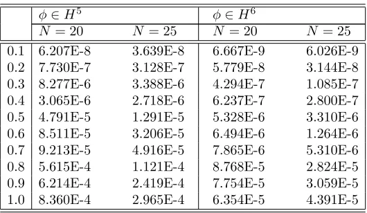
The absolute values of the errors are given in Table 1 for τi = _Ni, i = 1, . . . , N for

N = 20,25. From the numerical results, it is clear that the approximate solutions are in good agreement with the exact solution. Also it is clear form Tables 1 that by increasing the value ofrwe get the better results.

Table 1. Absolute ErroreN for Example 1.

ϕ∈H5 ϕ∈H6

N = 20 N = 25 N = 20 N= 25

(18)

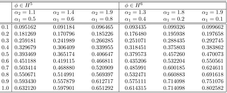
Table 2. Numerical solution using the technique given for 0≤τ≤1

and for diﬀerentα1 andα2 values.

ϕ∈H5 _ϕ_∈_H6

α2= 1.1 α2= 1.4 α2= 1.9 α2= 1.3 α2= 1.8 α2= 1.9

α1= 0.5 α1= 0.6 α1= 0.8 α1= 0.4 α1= 0.2 α1= 0.1

0.1 0.095162 0.091184 0.096465 0.093435 0.099326 0.099662

0.2 0.181269 0.170796 0.185226 0.176480 0.195938 0.197658

0.3 0.259181 0.241989 0.266285 0.251071 0.288435 0.292745

0.4 0.329679 0.306409 0.339955 0.318451 0.375803 0.383862

0.5 0.393469 0.365174 0.406647 0.379573 0.457260 0.470073

0.6 0.451188 0.419115 0.466811 0.435206 0.532204 0.550561

0.7 0.503414 0.468880 0.520909 0.485991 0.600185 0.624611

0.8 0.550671 0.514991 0.569397 0.532471 0.660883 0.691618

0.9 0.593430 0.557879 0.612717 0.575111 0.714098 0.751076

1.0 0.632120 0.597901 0.651292 0.614315 0.714098 0.802582

Example 7.2. Now, let us consider the following equation

Dα2

∗τϕ(τ) +D α1

∗τϕ(τ) = 0, (7.3)

D(0)ϕ(0) = 0, D(1)ϕ(0) = 1. (7.4)

where 1< α2≤2 and 0≤α1<1. The exact solution of this problem forα2= 2 and

α1 = 0 is ϕ(τ) = sin(τ). Using the proposed method, we choose 40 points in [0,1], and calculate the absolute errors inH5_and_H6_{, the computational errors are plotted} in Figure 1. The results show that the approximate solutions are in a good agreement with the exact solution whenα2 = 2 and α1 = 0. Table 2 shows the approximation values in some pointsτ∈[0,1] for diﬀerentα2andα1.

Example 7.3. We consider the following multi-order fractional diﬀerential equation of the form [31]

µ1Dα_∗τ2ϕ(τ) +µ2D_∗ατ1ϕ(τ) +µ3ϕ3(τ) =g(τ), (7.5)

D(0)ϕ(0) = 0, 0< α1< α2≤1, (7.6)

where

g(τ) = 2µ1τ 3−α2

Γ(4−α2)

+2µ2τ 3−α1

Γ(4−α1) +µ3τ

9

27 . (7.7)

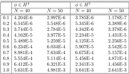
The exact solution of this equation is ϕ(τ) = τ3

3. The absolute values of the errors are given in Table 3 forτi= _Ni, i= 1, . . . , N forN = 40,50. From Table 3 we can see

(19)

Table 3. Absolute ErroreN for Example 3.

ϕ∈H4 ϕ∈H5

N = 40 N = 50 N = 40 N= 50

0.1 4.204E-6 2.997E-6 3.785E-6 1.178E-7 0.2 6.545E-6 5.548E-6 5.345E-6 3.389E-6 0.3 3.744E-5 2.784E-5 4.342E-6 3.378E-6 0.4 4.162E-5 3.977E-5 2.234E-5 1.431E-5 0.5 5.489E-5 5.259E-5 4.125E-5 2.256E-5 0.6 6.234E-4 6.034E-4 5.907E-5 3.542E-5 0.7 8.981E-4 7.634E-4 6.675E-4 5.157E-4 0.8 5.554E-4 5.114E-4 5.456E-4 4.871E-4 0.9 6.412E-3 6.321E-3 2.341E-3 1.456E-3 1.0 5.631E-3 4.981E-3 3.641E-3 2.641E-3

8. _{Concluding Remarks}

There are some main goals that we aimed by this work. The first is to present a relatively new semi-analytical technique to derive approximate analytical solution for nonlinear multi-order FDEs. The second is to addresse the sufficient conditions for uniqueness of solution and to study technique in differentRKHS. Furthermore, the numerical tests are presented to show the accuracy of the proposed technique. The numerical results demonstrate the relatively rapid convergence of the proposed technique. We should also point out that the example studied in the paper shows that the technique is very effective and convenient for solving nonlinear multi-order FDEs.

9. _{Acknowledgments}

The authors was partially supported by the Center of Excellence for Mathematics, University of Shahrekord.

References

[1] O. Abu Arqub, Mo. Al-Smadi, Sh. Momani, Application of reproducing kernel method for solving nonlinear Fredholm-Volterra integrodiﬀerential equations, Abstract and Applied Analysis, 2012, Article ID 839836, 16 pages, 2012.

[2] O. Abu Arqub, Mo. Al-Smadi, N. Shawagfeh, Solving Fredholm integro-diﬀerential equations using reproducing kernel Hilbert space method, Appl. Math. Comput., 219 (2013), 8938-8948. [3] B. Ahmad, G. Wang, A study of an impulsive four-point nonlocal boundary value problem of

nonlinear fractional diﬀerential equations, Comput. Math. Appl., 62(3) (2011), 1341-1349. [4] G. Akram, H.U. Rehman, Solution of ﬁrst order singularly perturbed initial value problem in

reproducing kernel Hilbert space, Eur. J. Sci. Res., 53(4) (2011), 516-523.

[5] G. Akram, H.U. Rehman, Numerical solution of eighth order boundary value problems in re-producing kernel space, Numerical Algorithms, 62(3) (2013), 527-540.

[6] N. Aronszajn, Theory of reproducing kernel. Trans. Amer. Math. Soc., 68 (1950), 337-404. [7] S. Badraoui, Approximate controllability of a reaction-diﬀusion system with a cross-diﬀusion

(20)

[8] R.L. Bagley, P.J. Torvik, A theoretical basis for the application of fractional calculus to vis-coelasticity, J. Rheol., 27 (1983), 201-210.

[9] R.L. Bagley, P.J. Torvik, On the appearance of the fractional derivative in the behavior of real materials, J. Appl. Mech. Asme., 51 (1984), 294-298.

[10] D. Baleanu, K. Diethelm, E. Scalas, J.J. Trujillo, Fractional calculus models and numerical methods, World Scientiﬁc, 2012.

[11] S. Bushnaq , Sh. Momani, Y. Zhou, A Reproducing Kernel Hilbert Space Method for Solving Integro-Diﬀerential Equations of Fractional Order, J. Optim. Theory Appl., 156 (2013), 96-105. [12] M.G. Cui, Y.Z. Lin, Nonlinear Numerical Analysis in the Reproducing Kernel Space, Nova

Science, New York, NY, USA, 2009.

[13] V. Daftardar-Gejji, S. Bhalekar, Solving multi-term linear and non-linear diﬀusion-wave equa-tions of fractional order by Adomian decomposition method, Appl. Math. Comput., 202(1) (2008), 113-120.

[14] V. Daftardar, H. Jafari, Solving a multi-order fractional diﬀerential equations using Adomian decomposition, Appl. Math. Comput., 189 (2007), 541-548.

[15] K. Diethelm, N.J. Ford, Multi-order fractional diﬀerential equations and their numerical solu-tion, Appl. Math. Comput., 154 (2004), 621-640.

[16] F. Geng, M. Cui, A reproducing kernel method for solving nonlocal fractional boundary value problems, Appl. Math. Lett., 25(5) (2012), 818-823.

[17] F. Geng, A novel method for solving a class of singularly perturbed boundary value problems based on reproducing kernel method, Appl. Math. Comput., 218(8) (2011), 4211-4215. [18] F. Geng, M. Cui, Homotopy perturbation-reproducing kernel method for nonlinear systems of

second order boundary value problems, J. Comput. Appl. Math., 235 (2011), 2405-2411. [19] A. Golbabai, K. Sayevand, The homotopy perturbation method for multi-order time fractional

diﬀerential equations, Nonlinear Sci. Lett. A, 2 (2013), 141-147.

[20] T.T. Hartley, C.F. Lorenzo, H.K. Qammer, Chaos in a fractional order Chua’s system, IEEE Transactions on Circuits and Systems I, 42(8) (1995), 485-490.

[21] I. Hashim, O. Abdulaziz, S. Momani, Homotopy analysis method for fractional IVPs, Commun. Nonlinear Sci. Numerical Simulation, 14(3) (2009), 674-684.

[22] W. Jiang, Y.Z. Lin, Approximate solution of the fractional advection-dispersion equation, Com-puter Physics Communications, 181(3) (2010), 557-561.

[23] S. Liang, J. Zhang, Existence and uniqueness of strictly nondecreasing and positive solution for a fractional three-point boundary value problem, Comput. Math. Appl., 62(3) (2011), 1333-1340. [24] F. Liu, P. Zhuang, V. Anh, I. Turner, K. Burrage, Stability and convergence of the diﬀer-ence methods for the space-time fractional advection-diﬀusion equation, Appl. Math. Comput., 191(1) (2007), 12-20.

[25] J.T. Machado, Discrete-time fractional-order controllers, Fractional Calculus & Applied Analy-sis, 4(1) (2001), 47-66.

[26] R.L. Magin, Fractional calculus in bioengineering, Critical Reviews in Biomedical Engineering, 32(1) (2004), 1112-1117.

[27] R.L. Magin, Fractional calculus in bioengineering, part 2, Critical Reviews in Biomedical Engi-neering, 32(2) (2004), 105-193.

[28] R.L. Magin, Fractional calculus in bioengineering, part 3, Critical Reviews in Biomedical Engi-neering, 32(3-4) (2004) 195-337.

[29] K. Miller, B. Ross, An introduction to the fractional calculus and fractional diﬀerential equa-tions, John Wiley & Sons, New York, NY, USA, 1993.

[30] M. Mohammadi, R. Mokhtari, Solving the generalized regularized long wave equation on the basis of a reproducing kernel space, J. Comput. Appl. Math., 235(14) (2011), 4003-4014. [31] R. Mokhtari, F. Toutian Isfahani, M. Mohammadi, Reproducing kernel method for solving

non-linear diﬀerential-diﬀerence equations, Abstract and Applied Analysis, 2012, Article ID 514103, 10 pages, 2012.

(21)

[33] S. Momani, M. Noor, Numerical methods for fourth-order fractional integro-diﬀerential equa-tions, Appl. Math. Comput., 182(1) (2006), 754-760.

[34] S. Momani, Z. Odibat, Analytical approach to linear fractional partial diﬀerential equations arising in ﬂuid mechanics, Physics Letters A, 355(4-5) (2006), 271-279.

[35] S. Momani, Z. Odibat, Numerical comparison of methods for solving linear diﬀerential equations of fractional order, Chaos, Solitons & Fractals, 31(5) (2007), 1248-1255.

[36] I. Petras, Chaos in the fractional-order Volta’s system: modeling and simulation, Nonlinear Dynamics, 57(1-2) (2009), 157-170.

[37] I. Podlubny, Fractional diﬀerential equations, Academic Press, New York, NY, USA, 1999. [38] Z. Odibat, S. Momani, Application of variational iteration method to nonlinear diﬀerential

equations of fractional order, I. J. Nonlinear Sciences and Numerical Simulation, 7(1) (2006), 27-34.

[39] M. Raberto, E. Scalas, F. Mainardi, Waiting-times and returns in high-frequency ﬁnancial data: an empirical study, Physica A, 314(1-4) (2002), 749-755.

[40] E.A. Rawashdeh, Numerical solution of fractional integro-diﬀerential equations by collocation method, Appl. Math. Comput., 176(1) (2006), 1-6.

[41] M. Rehman, R. Khan, Existence and uniqueness of solutions for multi-point boundary value problems for fractional diﬀerential equations, Appl. Math. Letters, 23(9) (2010), 1038-1044. [42] G. Samko, A.A. Kilbas, O.I. Marichev, Fractional integrals and derivatives, theory and

appli-cations, Gordon and Breach, Yverdon, 1993.

[43] E. Scalas, R. Gorenﬂo, F. Mainardi, Fractional calculus and continuous-time ﬁnance, Physica A, 284(1-4) (2000), 376-384.