Double Updating Online Learning

Double Updating Online Learning

Peilin Zhao [email protected]

Steven C.H. Hoi [email protected]

School of Computer Engineering Nanyang Technological University Singapore 639798

Rong Jin [email protected]

Department of Computer Science & Engineering Michigan State University

East Lansing, MI, 48824

Editor: Nicol`o Cesa-Bianchi

Abstract

In most kernel based online learning algorithms, when an incoming instance is misclassified, it will be added into the pool of support vectors and assigned with a weight, which often remains unchanged during the rest of the learning process. This is clearly insufficient since when a new support vector is added, we generally expect the weights of the other existing support vectors to be updated in order to reflect the influence of the added support vector. In this paper, we propose a new online learning method, termed Double Updating Online Learning, or DUOL for short, that explicitly addresses this problem. Instead of only assigning a fixed weight to the misclassified example received at the current trial, the proposed online learning algorithm also tries to update the weight for one of the existing support vectors. We show that the mistake bound can be improved by the proposed online learning method. We conduct an extensive set of empirical evaluations for both binary and multi-class online learning tasks. The experimental results show that the proposed technique is considerably more effective than the state-of-the-art online learning algorithms. The source code is available to public athttp://www.cais.ntu.edu.sg/˜chhoi/DUOL/.

Keywords: online learning, kernel method, support vector machines, maximum margin learning,

classification

1. Introduction

weights in order to fit in the constraint on the number of support vectors; in Kivinen et al. (2001), example weights are adjusted to deal with the drifting concepts.

Motivated by the above observations, we propose a new strategy for online learning that explic-itly addresses this problem. It is designed to dynamically tune the weights of support vectors in order to improve the classification performance. In some trials of online learning, besides assign-ing a weight to the misclassified example, the proposed online learnassign-ing algorithm also updates the weight for one of the existing support vectors, referred to as auxiliary example. We refer to the proposed approach as Double Updating Online Learning (Zhao et al., 2009), or DUOL for short.

The key challenge in the proposed online learning approach is to decide which existing support vector should be selected for updating weight. An intuitive choice is to select the existing support vector that “conflicts” with the new misclassified example, that is the existing support vector which on the one hand shares similar input pattern as the new example and on the other hand belongs to a class different from that of the new example. In order to quantitatively analyze the impact of updating the weight for such an existing support vector, we employ an analysis that is based on the work of online convex programming by incremental dual ascent (Shalev-Shwartz and Singer, 2006, 2007). Our analysis shows that under certain conditions, the proposed online learning algorithm can significantly reduce the mistake bound of the existing online algorithms. Besides binary classi-fication, we extend the double updating online learning algorithm to multi-class learning. Extensive experiments show promising performance of the proposed online learning algorithm compared to the state-of-the-art algorithms for online learning.

The rest of this paper is organized as follows. Section 2 reviews the related work for online learning. Section 3 presents the proposed “double updating” approach for online learning of binary classification problems. Section 4 extends the double updating method to online multi-class learn-ing. Section 5 gives our experimental results. Section 6 discusses the possible directions to explore in the future. Section 7 concludes this work.

2. Related Work

The proposed online learning algorithm is closely related to the recent work of online convex programming by incremental dual ascent (Shalev-Shwartz and Singer, 2006, 2007). Although the idea of simultaneously updating the weights of multiple support vectors was mentioned in Shalev-Shwartz and Singer (2006, 2007), neither efficient algorithm nor theoretical result was given explic-itly in their work. Besides, our work is also related to budget online learning (Weston and Bordes, 2005; Crammer et al., 2003; Cavallanti et al., 2007; Dekel et al., 2008) and online learning for drift-ing concepts. Although these online learndrift-ing algorithms are capable of dynamically adjustdrift-ing the weights of support vectors, they are designed to either fit in the budget for the number of support vectors or to handle drifting concepts, but not to reduce the number of classification mistakes in online learning.

Finally, several algorithms were proposed for online training of SVM that update the weights of more than one support vectors simultaneously (Cauwenberghs and Poggio, 2000; Bordes et al., 2005, 2007; Dredze et al., 2008; Crammer et al., 2008, 2009). In particular, in Bordes et al. (2005, 2007), the authors proposed to update the weights of two support vectors simultaneously at each iteration, similar to the proposed algorithm. These algorithms differ from the proposed one in that they are designed for efficiently learning an SVM classification model, not for online learning, and therefore do not provide guarantee for mistake bound.

3. Double Updating Online Learning for Binary Classification

In this section, we present the proposed double updating online learning method for solving online binary classification tasks. Below we start by introducing some preliminaries and notations.

3.1 Preliminaries and Notations

We consider the problem of online classification. Our goal is to learn a function f :Rd→Rbased on

a sequence of training examples{(x1,y1), . . . ,(xT,yT)}, where xt∈Rd is a d-dimensional instance

and yt ∈

Y

assignment for any x, and|f(x)|to measure the classification confidence. Letℓ(f(x),y):R×

Y

be the loss function that penalizes the deviation of estimates f(x)from observed labels y. We refer

to the output f of the learning algorithm as a hypothesis and denote the set of all possible hypotheses by

H

In this paper, we consider

H

kernel functionκ(·,·):Rd×Rd→R(Vapnik, 1998) implementing the inner producth·,·isuch that:

1)κhas the reproducing propertyhf,κ(x,·)i= f(x)for x∈Rd; 2)

H

H

X

1

2. To make it clear, we use

H

explicit dependence on kernel functionκ. Throughout the analysis, we assumeκ(x,x)≤1 for any

x∈Rd.

3.2 Motivation

We consider trial t in an online learning task where the training example(xa,ya)is misclassified (i.e., yaf(xa)≤0)). Let

D

predefined constant. The resulting classifier, denoted by f(x), is given by

f(x) =

n

∑

i=1

αiyiκ(x,xi).

In the conventional approach for online learning, we simply assign a constant weight, denoted by

β∈(0,C], to(xa,ya), and the resulting classifier becomes

f′(x) =βyaκ(x,xa) +

n

∑

i=1

αiyiκ(x,xi) =βyaκ(x,xa) +f(x).

The shortcoming of the conventional online learning approach is that the introduction of the new

support vector (xa,ya) may harm the classification of existing support vectors in

D

re-vealed by the following proposition.

Proposition 1 Let (xa,ya) be an example misclassified by the current classifier f(x) = ∑n

i=1αiyiκ(x,xi) with αi ≥0,i=1, . . . ,n, that is, yaf(xa) <0. Let f′(x) = βyaκ(x,xa) + f(x) be the updated classifier with β>0. There exists at least one support vector xi ∈

D

Proof It follows from the fact that:∃xi∈

D,

As indicated by Proposition 1, when a misclassified example(xa,ya)is added to the classifier, the

classification confidence of at least one existing support vector will be reduced. When yaf(xa)≤ −γ,

there exists one support vector (xb,yb)∈

D

vector will be misclassified by the updated classifier f′(x)if ybf(xb)≤βγ/n. In order to alleviate

this problem, we propose to update the weight for the existing support vector whose classification confidence is significantly affected by the new misclassified example. In particular, we consider a

support vector(xb,yb)∈

D

• ybf(xb)≤0, that is, support vector(xb,yb)is misclassified by the current classifier f(x);

• k(xb,xa)yayb ≤ −ρ where ρ∈(0,1) is a predetermined threshold, that is, support vector

(xb,yb)“conflicts” with the new misclassified example(xa,ya).

We refer to the support vector satisfying the above conditions as an auxiliary example. It is clear that by adding the misclassified example(xa,ya)to classifier f(x)with weightβ, the classification

score of(xb,yb)will be reduced by at leastβρ, which could lead to a significant misclassification of

the auxiliary example(xb,yb). To avoid such a mistake, we propose to update the weights for both

(xa,ya)and(xb,yb)simultaneously. In the next section, we show the details of the double updating

algorithm for online learning, and the analysis for mistake bound.

Our analysis follows closely the previous work on the relationship between online learning and the dual formulation of SVM (Shalev-Shwartz and Singer, 2006, 2007), in which the online learning is interpreted as an efficient updating rule for maximizing the objective function in the dual form

of SVM. We denote by∆t the improvement of the objective function in dual SVM when adding

a misclassified example to the classification function at the t-th trial. According to Theorem 1 in

all t,∆t is bounded from below by a bounding constant∆, then the number of mistakes made by

A

M≤ 1

∆ minf∈H_κ 1 2kfk

2

H_κ+C

T

∑

i=1

ℓ(yif(xi))

!

,

whereℓ(yif(xi)) =max(0,1−yif(xi))is the hinge loss function. According to Shalev-Shwartz and

Singer (2006, 2007), the bounding constant ∆=1/2 when we only update the classifier with the

newly misclassified example. In our analysis, we will show that ∆can be significantly improved

when updating the weights for both the misclassified example and the auxiliary example.

For the remaining part of this section, we denote by(xb,yb)an auxiliary example that satisfies

the two conditions specified before. We define

ka=κ(xa,xa),kb=κ(xb,xb),kab=κ(xa,xb),wab=yaybkab.

According to the assumption of auxiliary example, we have wab=kabyayb≤ −ρ. Finally, we denote

bybγb the weight for the auxiliary example(xb,yb)that is used in the current classifier f(x), byγa

andγbthe updated weights for(xa,ya)and(xb,yb), respectively, and by dγb the differenceγb−bγb.

3.3 Double Updating Online Learning for Binary Classification

Recall an auxiliary example(xb,yb)should satisfy two conditions (I) ybf(xb)≤0, and (II) wab≤ −ρ.

In addition, the example(xa,ya)received in the current iteration t is misclassified, that is, yaf(xa)≤

0. Following the framework of dual formulation for online learning, the following lemma shows

how to compute∆t, that is, the improvement in the objective function of dual SVM by adjusting

weights for(xa,ya)and(xb,yb).

Lemma 1 The maximal improvement in the objective function of dual SVM by adjusting weights for (xa,ya) and(xb,yb), denoted by ∆t, is computed by solving the following optimization prob-lem(which is a special case of the optimization problem (28) in Shalev-Shwartz and Singer, 2006):

∆t = max

γa,dγb

h(γa,dγb): 0≤γa≤C,−bγb≤dγb ≤C−bγb (1)

where

h(γa,dγb) =γa(1−yaf(xa)) +dγb(1−ybf(xb))−

ka

2γ

2 a−

kb

2d

2

γb−wabγadγb.

The lemma follows directly the dual formulation of SVM. The theorem below bounds the bounding

constant∆when C is sufficiently large.

Theorem 1 Assume C≥bγb+1/(1−ρ)withρ∈[0,1)for the selected auxiliary example(xb,yb), we have the following bound for the bounding constant∆:

∆≥ 1

1−ρ.

Proof First, we show dγb ≥0. This is because for givenγa≥0, the optimal solution for dγb, given

by

d_γb=1−ybf(xb)−wabγa

is positive because ybf(xb)≤0 and wab≤ −ρ. Using the fact ka,kb≤1,γa,dγb ≥0, yaf(xa)≤0,

ybf(xb)≤0, and wa,b≤ −ρ, we have

h(γa,dγb)≥γa+dγb−

1 2γ

2 a−

1 2d

2

γb+ργadγb.

Thus,∆is bounded as

∆≥ max

γb∈[0,C],dγb∈[0,C−bγb]

γa+dγb−

1 2(γ

2

a+d2γb) +ργadγb.

Under the condition that C≥ˆγ_b+1/(1−ρ), it is easy to verify that the optimal solution for the

above problem isγa=dγb=1/(1−ρ), which leads to the result in the theorem.

We refer to the case as a strong double update when the condition of Theorem 1 is satisfied. We

have the following theorem for the general case when we only have C≥1.

Theorem 2 Assume C≥1. We have the following bound for∆ when updating the weight for the misclassified example(xa,ya)and the auxiliary example(xb,yb):

∆≥1

2+

1

2min (1+ρ)

2_,(C−bγ)2_. Proof By settingγa=1, we have h(γa,dγb)computed as

h(γa=1,dγb)≥

1

2+ (1+ρ)dγb−

1 2d

2

γb.

Hence,∆is lower bounded by

∆≥1

2+dγb∈max[0,C−bγ]

(1+ρ)d_γb−1

2d

2

γb

≥1

2+

1

2min((1+ρ)

2_,(C−bγ)2_).

Although Theorem 1 and 2 show that the double update strategy could significantly improve

the bounding constant∆ over 1/2 and consequentially reduce the mistake bound, it is applicable

only when there exists an auxiliary example. Below, we extend the double update strategy to the cases when there is no auxiliary example. Specifically, we relax the condition for performing double update as follows: there exists(xb,yb)∈

D

We refer to these cases as weak double update.

Theorem 3 Assume wab≤ −ρ, ybft−1(xb)≤1 and C≥ˆγb+ρ, we have the following bound for the bounding constant

∆≥1+ρ

2

2 .

Proof Following the definitions and assumptions, we have ∆=max

γa,dγb

h(γa,dγb)≥h(1,ρ)≥1−

1

2+0−

ρ2

2 +ρ

2₌1+ρ2

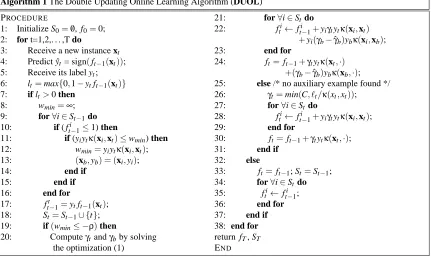
Algorithm 1 The Double Updating Online Learning Algorithm (DUOL)

PROCEDURE

1: Initialize S0=/0, f0=0;

2: for t=1,2,. . . ,T do

3: Receive a new instance xt 4: Predict ˆyt= sign(ft−1(xt)); 5: Receive its label yt; 6: lt=max{0,1−ytft−1(xt)} 7: if lt>0 then

8: wmin=∞; 9: for∀i∈St−1do

10: if ( f_ti₋₁≤1) then

11: if (yiytκ(xi,xt)≤wmin) then 12: wmin=yiytκ(xi,xt); 13: (xb,yb) = (xi,yi);

14: end if

15: end if

16: end for

17: f_tt₋₁=ytft−1(xt); 18: St=St−1∪ {t};

19: if(wmin≤ −ρ)then

20: Computeγtandγbby solving the optimization (1)

21: for∀i∈Stdo

22: fti← fti−1+yiγtytκ(xi,xt) +yi(γb−ˆγb)ybκ(xi,xb);

23: end for

24: ft=ft−1+γtytκ(xt,·) +(γb−γˆb)ybκ(xb,·);

25: else /* no auxiliary example found */

26: γt=min(C, ℓt/κ(xt,xt)); 27: for∀i∈Stdo

28: fi

t← fti−1+yiγtytκ(xi,xt);

29: end for

30: ft= ft−1+γtytκ(xt,·);

31: end if

32: else

33: ft=ft−1; St=St−1;

34: for∀i∈Stdo

35: fi

t← fti−1;

36: end for

37: end if

38: end for return fT, ST END

Figure 1: The Algorithms of Double Updating Online Learning (DUOL).

Solving the optimization problem (1) is the key to the double update. The following proposition provides the optimal solution to the problem (1).

Proposition 2 Denoteℓa:=1−yaf(xa)andℓb:=1−ybf(xb). Assume ℓa, ℓb≥0, ka,kb>0 and

wab≤0, then the solution of optimization problem (1) is as follows:

(γa,dγb) =

          

(C,C−γˆ_b) if(kaC+wab(C−γˆb)−ℓa)<0 and(kb(C−γˆb) +wabC−ℓb)<0 (C,ℓb−wabC

kb ) if

w2

abC−wabℓb−kakbC+kbℓa

kb >0 and ℓb−wabC

kb ∈[−ˆγb,C−ˆγb] (ℓa−wab(C−ˆγb)

ka ,C−ˆγb) if

ℓa−wab(C−ˆγb)

ka ∈[0,C]andℓb−kb(C−γˆb)−wab

ℓa−wab(C−γˆb)

ka >0 (kbℓa−wabℓb

kakb−w2ab

,kaℓb−wabℓa

kakb−w2ab

)if(kbℓa−wabℓb kakb−w2ab

,kaℓb−wabℓa

kakb−w2ab

)∈[0,C]×[−γˆ_b,C−ˆγ_b]

.

The detailed proof for Proposition 2 can be found in Appendix A. Figure 1 summarizes the proposed Double Updating Online Learning (DUOL) algorithm. In this algorithm, to efficiently find the

auxiliary example(xb,yb), we introduce a variable fti for each support vector to keep track of its

classification score. Parameterρis used to trade off between efficiency and efficacy for DUOL: the

smallerρthe more double updates will be performed.

Finally, we give the mistake bound for the DUOL algorithm. We denote by

M

that correspond to the trials of misclassification, that is,

In addition, we denote by

M

d(ρ)and

M

double updating, respectively, that is,

M

1

1−ρfor(xt,yt),t∈

M

M

M

Note that in set

M

d(ρ), for the convenience of analysis, we only consider the subset of strong

updates when the condition C≥bγb+1/(1−ρ) is satisfied. Finally, we denote the cardinalities of

sets

M

M

d, and

M

M

M

M

Mw_d(ρ), respectively.

Theorem 4 Let(x1,y1), . . . ,(xT,yT)be a sequence of examples, where xt ∈Rd,yt ∈ {−1,+1}and

κ(xt,xt)≤1 for all t, and assume C≥1. Then for any function f in

H

mistakes M made by DUOL on this sequence of examples is bounded by:

2 min

f∈H_κ 1 2kfk

2

H_κ+C

T

∑

i=1

ℓ(yif(xi))

! −ρ

2

2 M

w d(ρ)−

1+ρ

1−ρM

s d(ρ),

whereρ∈[0,1).

Proof According to Theorem 1 and 3, we have

min

t∈Ms d(ρ)

∆t ≥

1

1−ρ,t∈minMw d(ρ)

∆t≥

1+ρ2

2 .

Moreover, according to Theorem 2, we have∆t≥1/2,∀t∈

M

1

2Ms+

1+ρ2

2 M

w d(ρ) +

1

1−ρM

s

d(ρ)≤ min f∈H_κ

1 2kfk

2

H_κ+C

T

∑

i=1

ℓ(yif(xi))

!

.

We complete the proof using M=Ms+M_dw(ρ) +M_ds(ρ).

As revealed by the above theorem, the number of mistakes made by the proposed double updat-ing online learnupdat-ing algorithm will be smaller than the online learnupdat-ing algorithm that only performs a single update in each trial. The difference in the mistake bound is essentially due to the double updating, that is, the more the number of double updates, the more advantageous the proposed algo-rithm will be. Besides, the above bound also indicates that a strong double update is more powerful

than a weak double update given that the associated weight of a strong double update(1+ρ)/(1−ρ)

is always much larger than that of a weak double updateρ2_{/2. It is worthwhile pointing out that}

al-though according to Theorem 4, it seems that the larger the value ofρthe smaller the mistake bound

will be. This however may not be true because M_ds(ρ)in general decreases asρincreases. Finally,

we note that Theorem 4 bounds the number of mistakes made by the proposed DUOL algorithm

for C≥1. When C<1, the mistake bound for the proposed algorithm follows Theorem 2, 3 and

4. Multiclass Double Updating Online Learning

In this section, we extend the proposed double updating online learning algorithm to multiclass learning where each instance can be assigned to multiple classes.

4.1 Online Multiclass Learning

Similar to online binary classification, online multiclass learning is performed over a sequence of training examples (x1,Y1), . . . ,(xT,YT). Unlike binary classification where yt ∈ {−1,+1}, in

multi-class learning, each class assignment Yt ⊆

Y

making it a more challenging problem. We use ˆYt to represent the class set predicted by the online

learning algorithm. Before presenting our algorithm, we first review online multiclass learning (Crammer and Singer, 2003; Fink et al., 2006) based on the framework of label ranking (Crammer and Singer, 2005).

4.1.1 LABELRANKING FORMULTICLASSLEARNING

Given an instance x, the label ranking approach first computes a score for every class label in

Y

and ranks the classes in the descending order of their scores. The predicted class set ˆYt is formed by

the classes with the highest scores. The objective of label ranking is to ensure that the score of class

r is significantly larger than that of class s if r∈Yt is a true class assignment while s∈

Y

An instance x is classified incorrectly if that above condition is NOT satisfied.

We follow the protocol of multi-prototype (Vapnik, 1998; Crammer and Singer, 2001; Crammer et al., 2006) for the design of multiclass multilabel learning algorithm. It learns multiple

hypothe-ses/classifiers, one classifier for each class in

Y

the classification task. Specifically, for trial t, upon receiving an instance xt, the scores of k classes

output by the set of k hypotheses are given by

¯

ft−1(xt) = (ft−1,1(xt),· · ·,ft−1,k(xt))T,

where ft−1,i∈

H

rt=arg min

r∈Yt

ft−1,r(xt) and st=arg max s6∈Yt

ft−1,s(xt), (2)

here, rt and strepresent the class of the smallest score among all relevant classes and the class of the

largest score among the irrelevant classes, respectively. Using the notation of rt and st, the margin

with respect to the hypothesis set ¯ft−1at trial t is defined as follows: Γ _ft¯_{−1;(xt,Yt)= ft−1,r}

t(xt)−ft−1,st(xt).

Based on the notation of classification margin, we define the loss function of hypotheses ¯ft−1(x)for

training example(xt,Yt)as follows:

ℓ _f¯_{t−1;(xt,Yt) = max}

r∈Yt,s6∈Yt

1−(ft−1,r(xt)−ft−1,s(xt))

+,

4.1.2 A PERCEPTRONALGORITHM FORONLINE MULTICLASSLEARNING

According to Crammer and Singer (2003), when an example is misclassified at trial t, we update

each component of the classifier ¯ft−1as follows:

ft,i(x) = ft−1,i(x) +σYt(i,t)γtκ(xt,x),∀i∈

Y

whereγt ∈(0,C], and functionσYt(i,t), which is simplified asσ(i,t), is defined below:

σ(i,t) =

  

1 if i=rt

−1 if i=st

0 otherwise

.

Using notation H(Yt) = σ(1,t),· · ·,σ(k,t)

T

, we rewrite Equation (3) as ¯ft(x) = f¯t−1(x)+

γtH(Yt)κ(xt,x), or equivalently

¯

f(x) =

n

∑

i=1

γiH(Yi)κ(xi,x),

where n is the number of support vectors received so far.

4.2 Multiclass DUOL Algorithm

We extend the DUOL algorithm to multiclass learning. We denote by (xa,Ya) the misclassified

example received at the current trial, that is,(f¯(xa))ra−(f¯(xa))sa ≤0. Similar to DUOL for binary

classification, we introduce an auxiliary example(xb,Yb)from the existing support vectors that obey

the following conditions:

1. (f¯(xb))rb−(f¯(xb))sb ≤0, that is,(xb,Yb)is misclassified by current classifier ¯f ;

2. (H(Ya)·H(Yb))κ(xa,xb)≤ −2ρwhereρ∈(0,1)is a threshold. This property indicates that

example(xa,Ya)conflicts with example(xb,Yb).

Compared to auxiliary example defined for binary classification, we introduce H(Ya)·H(Yb) in

above when defining two conflicting instances. Givenκ(xa,xb)≥0, the second condition of

aux-iliary example implies H(Ya)·H(Yb)≤0, which further indicates that two examples (xa,Ya) and

(xb,Yb) have the opposite prediction, that is, (ra=sb) or (sa=rb). This result is revealed by the

following proposition.

Proposition 3 The inequality H(Ya)·H(Yb)<0 holds if and only if (ra=sb) or (sa=rb).

The proof of Proposition 3 is given in the appendix.

Similar to the DUOL algorithm for binary classification, our analysis aims to show that by updating weights for both misclassified example and the auxiliary example, we may be able to

significantly improve the bounding constant∆, which is defined as follows:

M×∆≤min

¯ f∈H¯κ

F(_f¯_{) +C}

∑

i=1

ℓ _{f ;}¯ _{(xi,Yi), (4)}

where ¯

H

H

H_κ. To ease our further discussions, we define ka=

κ(xa,xa),kb=κ(xb,xb),wab= (H(Ya)·H(Yb))κ(xa,xb).

The following proposition shows the optimization problem related to the multiclass double

Proposition 4 With the double updating, that is, adjusting the weight of some auxiliary support vector(xb,Yb)from ˆγbtoγb(denoted by dγb =γb−ˆγb) and assigning weightγa to the current

mis-classified example(xa,Ya), the improvement in the objective function of dual SVM, denoted by∆t, is computed by the following optimization problem:

max

γa,dγb

γa

1− ft−1,ra(xa)−ft−1,sa(xa)

+dγb

1− ft−1,rb(xb)−ft−1,sb(xb)

−kaγ2a−kbdγ2b−wabγadγb, (5)

s.t. 0≤γa≤C,−γˆb≤dγb≤C−γˆb.

Theorem 5 Assumeκ(x,x)≤1 for any x and C≥γˆb+₂₍₁1_−ρ) for the selected auxiliary example

(xb,Yb), we have the following bound for∆:

∆≥ 1

2(1−ρ).

We refer to the case as a strong double update when there exists a auxiliary example(xb,Yb) s.t.

C≥γˆb+₂₍₁1_−ρ). Similar to double updating for binary classification, we introduce weak double

update when there exists(xb,Yb)s.t. wab≤ −2ρ, ft−1,rb(xb)−ft−1,sb(xb)≤1, and C≥γˆb+ ρ

2. Theorem 6 Assume there exists (xb,Yb) s.t. wab≤ −2ρ, ft−1,rb(xb)−ft−1,sb(xb)≤1, C≥γˆb+

ρ

2 and the current instance is misclassified, then we have the following bounding constant

∆≥1+ρ

2

4 .

The exact solution to the Quadratic Programming (QP) problem in (5) is given by the following proposition.

Proposition 5 Denoteℓa:=1−(ft−1,ra(xa)−ft−1,sa(xa))andℓb:=1−(ft−1,rb(xb)−ft−1,sb(xb)).

Assumeℓa, ℓb≥0, ka,kb>0 and wab≤0, then the solution of optimization (5) is as follows:

(γa,dγb)=

          

(C,C−γˆ_b) if(2kaC+wab(C−ˆγb)−ℓa)<0 and(2kb(C−γˆb) +wabC−ℓb)<0 (C,ℓb−wabC

2kb ) if

w2_abC−wabℓb−4kakbC+2kbℓa

2kb >0 and ℓb−wabC

2kb ∈[−γˆb,C−γˆb] (ℓa−wab(C−ˆγb)

2ka ,C−ˆγb) if

ℓa−wab(C−ˆγb)

2ka ∈[0,C]andℓb−2kb(C−γˆb)−wab

ℓa−wab(C−ˆγb)

2ka >0 (2kbℓa−wabℓb

4kakb−w2ab

,2kaℓb−wabℓa

4kakb−w2ab

)if(2kbℓa−wabℓb

4kakb−w2ab

,2kaℓb−wabℓa

4kakb−w2ab

)∈[0,C]×[−ˆγb,C−ˆγb]

.

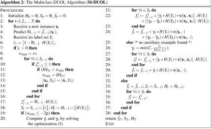
We skip the proof due to its high similarity to that of Proposition 2. Figure 2 summarizes the steps of the multiclass DUOL (M-DUOL) algorithm. Note that we replace the conditions for auxiliary example with the margin error in order to make more double updates.

A mistake bound for the M-DUOL algorithm, similar to Theorem 4, is given by the following theorem.

Theorem 7 Let (x1,Y1), . . . ,(xT,YT) be a sequence of examples, where xt ∈ Rn, Yt ⊆

Y

H

4

min

¯ f∈H¯_κ

F(_f¯_{) +C}

∑

i=1

ℓ _{f ;}¯ _(xi,Yi)−ρ2

2 M

w d(ρ)−

1+ρ

1−ρM

Algorithm 2: The Multiclass DUOL Algorithm (M-DUOL)

PROCEDURE

1: Initialize H0=/0, S0=/0, ¯f0=0;

2: for t=1,2,. . . ,T do

3: Receive a new instance xt 4: Predict Wt−1=f¯t−1(xt); 5: Receive its label set Yt 6: ℓt=

1−Wt−1·H(Yt)]+

7: if lt>0 then 8: wmin=∞; 9: for∀i∈St−1do

10: if fi

t−1≤1 then

11: if(Hkti<wminthen

12: wmin=Hkti;

13: (xb,Yb) = (xi,Yi);

14: end if

15: end if

16: end for

17: f_tt₋₁=Wt−1·H(Yt); 18: St=St−1∪

t ; Ht=Ht−1∪

H(Yt) ; 19: if(wmin≤ −2ρ)then

20: Computeγtandγbby solving the optimization (5)

21: for∀i∈Stdo

22: fti← fti−1+ [γt∗H(Yt)∗κ(xt,xi)]·H(Yi) + [(γb−γˆb)∗H(Yb)∗κ(xb,xi)]·H(Yi);

23: end for

24: f¯t= f¯t−1+γt∗H(Yt)∗κ(xt,·) + (γb−γˆb)∗H(Yb)∗κ(xb,·);

25: else /* no auxiliary example found */

26: γt=min(C,_2κ(ℓ_xt_t,xt)); 27: for∀i∈Stdo

28: fti←fti−1+ [γt∗H(Yt)∗κ(xt,xi)]·H(Yi);

29: end for

30: f¯t= f¯t−1+γt∗H(Yt)∗κ(xt,·);

31: end if

32: else

33: f¯t=f¯t−1; St=St−1; Ht=Ht−1;

34: for∀i∈Stdo 35: fti← fti−1;

36: end for

37: end if

38: end for return ¯fT, ST, HT END

Figure 2: Algorithms of multiclass double-updating online learning (M-DUOL).

5. Experimental Results

In this section, we evaluate the empirical performance of the proposed double updating online learn-ing algorithms for online learnlearn-ing tasks. We first evaluate the performance of DUOL for binary classification, followed by the evaluation of multiclass double updating online learning.

5.1 Testbeds and Experimental Setup for Binary-class Online Learning

We compare our technique with a number of state-of-the-art techniques, including the kernel Per-ceptron algorithm (Kivinen et al., 2001), the “ROMMA” algorithm and its aggressive version

“agg-ROMMA” (Li and Long, 1999), the ALMAp(α) algorithm (Gentile, 2001), and the

Passive-Aggressive algorithms (“PA”) (Crammer et al., 2006). For PA, two versions of algorithms (PA-I and PA-II) are implemented as described in Crammer et al. (2006). Note that one may also compare with the online SVM algorithm (Shalev-Shwartz and Singer, 2006), which updates the weights for all support vectors in each trial. However, we do not include this baseline for compari-son because it is too computationally intensive to run on some large data sets.

For the proposed DUOL algorithms, we implement three variants based on different solvers to

the problem in (1): (i) “DUOLappr” that employs an approximate solution to (1), that is,γt =₁₋1_ρ

andγb=ˆγb+₁₋1_ρ, (ii)“DUOL” that uses the exact solution to (1) given in Proposition 2, and (iii)

“DUOLiter” that first updates the weight for the misclassified example and then the weight for

We test all the algorithms on eight benchmark data sets from web machine learning repositories,

which are listed in table 1. All of the data sets can be downloaded from LIBSVM website,1 UCI

machine learning repository,2and MIT CBCL face data sets.3

Data Set # examples # features

sonar 208 60

splice 1,000 60

german 1,000 24

mushrooms 8,124 112

dorothea 1,150 100,000

spambase 4,601 57

MITFace 6,977 361

w7a 24,692 300

Table 1: Binary-class data sets used in the experiments.

To make a fair comparison, for all algorithms in comparison, we set C =5 and use the same

Gaussian kernel withσ=8. For the ALMAp(α)algorithm, parameter p andαare set to 2 and 0.9,

respectively, based on our experience. For the proposed DUOL algorithm, we fixρto be 0 for all

cases. All the experiments are repeated 20 times, each with an independent random permutation of the data points. All the results are reported by averaging over the 20 runs. We evaluate the online learning performance by measuring the mistake rate, that is, the percentage of examples that are misclassified by the online learning algorithm. We measure the sparsity of the learned classifiers by the number of support vectors. We evaluate computational efficiencies of all the algorithms in terms of their CPU running time (in seconds). All the experiments are run in Matlab over a windows machine of 2.3GHz CPU.

5.2 Performance Evaluation for Binary-Class Online Learning

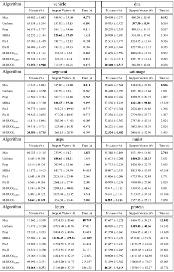
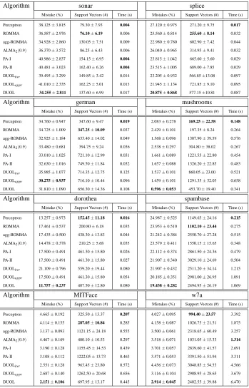
Table 2 summarizes the performance of all the compared online learning algorithms over the binary data sets. We can draw several observations from the results.

First, among the six baseline algorithms in comparison, we observe that the agg-ROMMA and two PA algorithms (PA-I and PA-II) perform considerably better than the other three algorithms (i.e., Perceptron, ROMMA, and ALMA) in most cases. We also notice that the agg-ROMMA and the two PA algorithms consume considerably larger numbers of support vectors than the other three algorithms. We believe this is because the agg-ROMMA and the two PA algorithms adopt more aggressive strategies than the other three algorithms, resulting in more updates and better classification performance. For the convenience of discussion, we refer to agg-ROMMA and two PA algorithms as aggressive algorithms, and the other three online learning algorithms as

non-aggressive ones.

Second, we observe that among the three variants of double updating online learning, the DUOL approach, which solves the optimization problem exactly, yields the least mistake rate with the smallest number of support vectors for most of the cases. Comparing with the baseline algorithms,

Algorithm sonar splice

Mistake (%) Support Vectors (#) Time (s) Mistakes (%) Support Vectors (#) Time (s)

Perceptron 38.125±3.815 79.30±7.93 0.004 27.120±0.975 271.20±9.75 0.017

ROMMA 36.587±2.976 76.10±6.19 0.006 25.560±0.814 255.60±8.14 0.032 agg-ROMMA 34.928±2.860 130.05±7.51 0.009 22.980±0.780 602.90±7.42 0.044 ALMA2(0.9) 36.370±3.572 86.25±6.43 0.006 26.040±0.965 314.95±9.41 0.032 PA-I 40.986±2.837 154.15±6.95 0.004 23.815±1.042 665.60±5.60 0.029 PA-II 40.481±3.023 162.40±6.26 0.004 23.515±1.005 689.00±7.85 0.029 DUOLiter 39.495±3.299 149.85±3.42 0.014 23.205±0.932 566.85±13.08 0.097

DUOLappr 41.010±2.335 162.25±5.01 0.013 21.945±1.134 721.85±9.10 0.095

DUOL 34.255±2.811 137.60±6.99 0.017 20.875±0.868 577.15±10.81 0.087

Algorithm german mushrooms

Mistake (%) Support Vectors (#) Time (s) Mistakes (%) Support Vectors (#) Time (s)

Perceptron 34.760±0.947 347.60±9.47 0.019 2.083±0.278 169.25±22.58 0.148

ROMMA 34.725±1.009 347.25±10.09 0.037 2.429±0.101 197.35±8.24 0.264 agg-ROMMA 32.925±1.184 633.40±14.02 0.049 1.568±0.096 1307.90±39.59 0.576 ALMA2(0.9) 33.480±0.681 394.75±9.24 0.036 2.538±0.297 304.80±38.02 0.267 PA-I 33.010±1.025 721.10±12.99 0.031 1.661±0.089 1221.55±22.80 0.454 PA-II 32.630±1.016 749.50±11.84 0.032 1.657±0.088 1326.20±22.85 0.483 DUOLiter 35.985±1.077 714.35±12.75 0.125 1.537±0.101 860.05±23.00 0.521

DUOLappr 30.275±0.937 716.10±10.44 0.096 1.459±0.101 1291.35±32.03 0.658

DUOL 31.810±1.090 656.30±14.36 0.108 0.596±0.053 453.70±19.40 0.341

Algorithm dorothea spambase

Mistake (%) Support Vectors (#) Time (s) Mistakes (%) Support Vectors (#) Time (s)

Perceptron 13.257±0.973 152.45±11.18 0.016 24.987±0.525 1149.65±24.16 0.215

ROMMA 17.461±0.537 200.80±6.18 0.035 23.953±0.510 1102.10±23.44 0.275 agg-ROMMA 17.435±0.500 438.30±13.83 0.044 21.242±0.384 2550.70±27.28 0.515 ALMA2(0.9) 14.478±0.378 210.25±5.68 0.035 23.579±0.411 1550.15±15.65 0.348 PA-I 17.500±0.491 461.30±15.80 0.026 22.112±0.374 2861.50±24.36 0.479 PA-II 17.500±0.491 461.30±15.80 0.027 21.907±0.340 3029.10±24.69 0.504 DUOLiter 21.109±0.796 559.20±19.44 0.080 21.907±0.432 2511.20±34.14 1.215 DUOLappr 17.500±0.491 461.30±15.80 0.054 20.185±0.351 2981.00±26.95 1.091

DUOL 11.757±0.237 407.50±12.80 0.080 19.438±0.282 2494.95±26.19 1.069

Algorithm MITFace w7a

Mistake (%) Support Vectors (#) Time (s) Mistakes (%) Support Vectors (#) Time (s)

Perceptron 4.665±0.192 325.50±13.37 0.207 4.027±0.095 994.40±23.57 3.392 ROMMA 4.114±0.155 287.05±10.84 0.285 4.158±0.087 1026.75±21.51 1.875 agg-ROMMA 3.137±0.093 1121.15±24.18 0.555 3.500±0.061 2318.65±60.49 3.257 ALMA2(0.9) 4.467±0.169 400.10±10.53 0.297 3.518±0.071 1031.05±15.33 1.314 PA-I 3.190±0.128 1155.45±14.53 0.439 3.701±0.057 2839.60±41.57 2.691 PA-II 3.108±0.112 1222.05±13.73 0.463 3.571±0.053 3391.50±51.94 3.311 DUOLiter 2.551±0.128 963.45±23.80 0.572 4.456±0.073 3048.85±54.53 4.566

DUOLappr 2.687±0.140 1262.50±20.68 0.656 3.116±0.104 2908.95±28.65 3.679

DUOL 2.151±0.106 697.95±13.17 0.445 2.914±0.045 2402.55±39.88 6.470

we observe that DUOL achieves significantly smaller mistake rates than the other single-updating algorithms in all cases. This shows that the proposed double updating approach is effective in im-proving the performance of online prediction. By examining the number of support vectors, we observed that DUOL results in sparser classifiers than the three aggressive online learning algo-rithms, and denser classifiers than the three non-aggressive algorithms.

Third, according to the results of running time, we observe that DUOL is overall efficient as compared with the state-of-the-art online learning algorithms. Among all the algorithms in compar-ison, Perceptron, due to its simplicity nature, is clearly the most efficient algorithm. Since DUOL requires double updates, it is less efficient than PA, ROMMA and ALMA algorithms, but is compa-rable to the agg-ROMMA algorithm. Note that the comparisons of running time costs are slightly different compared with the results in our previous conference paper (Zhao et al., 2009) because we did some improvements of efficiency for the implementations of some existing algorithms in this journal article.

5.3 Evaluation of Different Auxiliary Example Selection Strategies and the Sensitivity to Parameter C for DUOL

As the performance of DUOL quite relies on the choice of auxiliary examples, in this section, we evaluate different auxiliary example selection strategies. Specifically, we compare the proposed

strategy to a random selection approach, referred to as “DUOLrand”, which randomly chooses an

auxiliary example from the existing support vectors. The exact solution to the problem in (1), given

by Proposition 2, is used for updating the weights of both examples. We setρ=0 andσ=8 for all

the data sets, same as the previous experiments.

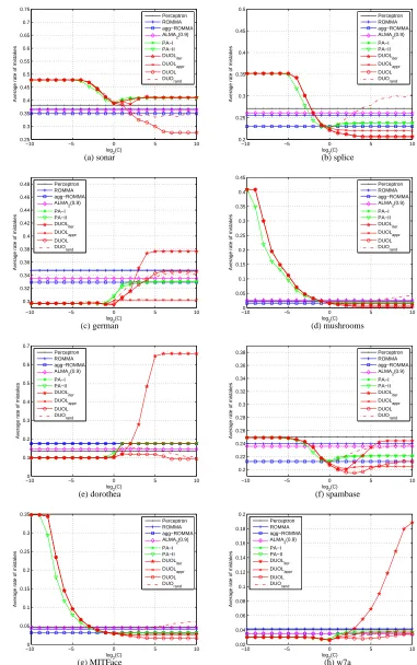
Figure 3 compares the online prediction performance between DUOL and DUOLrand as well

as the other competing algorithms with varied C values across eight different data sets. Several observations can be drawn from the results.

First, it is clear to see that the proposed strategy for selecting auxiliary examples is more effec-tive than the random selection strategy for most cases. Second, among all the compared algorithms, we observe that DUOL always achieves the best performance when C is sufficiently large (e.g.,

C>10), except for data sets “german” and “w7a” where a smaller C value tends to produce a better

result. This observation is consistent to our previous theoretical result, which indicates setting a large C value usually implies more strong updates and consequently a better mistake bound. Third, we observe that the proposed DUOL algorithm is significantly more accurate than the other two

variants of double updating online learning algorithms (DUOLiterand DUOLappr) for varied C

val-ues, as we expected. We observe that DUOLiter, the iterative updating approach, performs unstably,

which might be due to local optimum suffered from its heuristic update. This observation validates the importance of performing the optimal double updates by the proposed DUOL algorithm.

5.4 Empirical Evaluation of Mistake Bounds

To examine how the double updating strategy affects the mistake bound, we empirically compare M,

the total number of mistakes made by the DUOL algorithm, Mw_d(ρ), the number of mistake cases

where the weak double updates are applied, and Ms

d(ρ), the number of mistake cases where the

strong double updates are applied. Figure 4 shows the comparison between M, Mw_d(ρ), and Ms

d(ρ)

−10 −5 0 5 10 0.25 0.3 0.35 0.4 0.45 0.5 0.55 0.6 0.65 0.7 0.75

log₂(C)

Average rate of mistakes

Perceptron ROMMA agg−ROMMA ALMA₂(0.9) PA−I PA−II DUOL iter DUOL_appr DUOL DUO_rand

−10 −5 0 5 10

0.2 0.25 0.3 0.35 0.4 0.45 0.5

log₂(C)

Average rate of mistakes

Perceptron ROMMA agg−ROMMA ALMA₂(0.9) PA−I PA−II DUOL iter DUOL_appr DUOL DUO_rand

(a) sonar (b) splice

−10 −5 0 5 10

0.3 0.32 0.34 0.36 0.38 0.4 0.42 0.44 0.46 0.48

log₂(C)

Average rate of mistakes

Perceptron ROMMA agg−ROMMA ALMA 2(0.9) PA−I PA−II DUOL iter DUOL_appr DUOL DUO_rand

−100 −5 0 5 10

0.05 0.1 0.15 0.2 0.25 0.3 0.35 0.4 0.45

log₂(C)

Average rate of mistakes

Perceptron ROMMA agg−ROMMA ALMA 2(0.9) PA−I PA−II DUOL iter DUOL_appr DUOL DUO_rand

(c) german (d) mushrooms

−100 −5 0 5 10

0.1 0.2 0.3 0.4 0.5 0.6 0.7

log₂(C)

Average rate of mistakes

Perceptron ROMMA agg−ROMMA ALMA 2(0.9) PA−I PA−II DUOL iter DUOL appr DUOL DUO_rand

−10 −5 0 5 10

0.2 0.22 0.24 0.26 0.28 0.3 0.32 0.34 0.36 0.38

log₂(C)

Average rate of mistakes

Perceptron ROMMA agg−ROMMA ALMA 2(0.9) PA−I PA−II DUOL iter DUOL appr DUOL DUO_rand

(e) dorothea (f) spambase

−100 −5 0 5 10

0.05 0.1 0.15 0.2 0.25 0.3 0.35

log₂(C)

Average rate of mistakes

Perceptron ROMMA agg−ROMMA ALMA 2(0.9) PA−I PA−II DUOL_iter DUOL appr DUOL DUO rand

−10 −5 0 5 10

0.02 0.04 0.06 0.08 0.1 0.12 0.14 0.16 0.18 0.2

log₂(C)

Average rate of mistakes

Perceptron ROMMA agg−ROMMA ALMA 2(0.9) PA−I PA−II DUOL_iter DUOL appr DUOL DUO rand

(g) MITFace (h) w7a

First, we observe that double updates are frequently applied whenρis small. This is because

it is easier to find an auxiliary example for double updating whenρis small. Further, we find that

settingρclose to 0 by default often leads to the best or close to the best results. Second, we observe

that the number of weak updates is significantly larger than that of strong updates. This is because the condition of conducting a strong double update is significantly more difficult to be satisfied

that that for a weak double update. Third, we observe that both M_dw(ρ)and Ms_d(ρ)monotonically

decrease when increasing the value ofρ. In the extreme case, whenρis close to 1, their value often

drops to zero, indicating that no double update was applied. In the meantime, we find that the total

number of mistakes often reaches the maximum, asρapproaches 1. These results again validate the

importance and effectiveness of the proposed double updating algorithm.

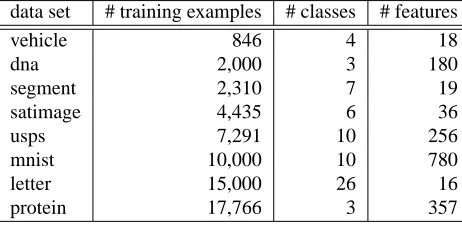
5.5 Testbeds and Experimental Setup for Multiclass Online Learning

Table 3 shows the multiclass data sets from Web machine learning repository used in our experi-ments. We compare the proposed M-DUOL algorithm with six state-of-the-art online learning algo-rithms. The first three algorithms are variants of Perceptron-based on methods studied in Crammer and Singer (2003). They are: (i) “Max”, the perceptron method based on the max-score multiclass update, (ii) “Uniform”, the perceptron method based on the Uniform multiclass update, and (iii) “Prop”, the perceptron method based on the proportion multiclass update. We also compare the proposed algorithm with the other three state-of-the-art online multi-class learning algorithms, in-cluding the MIRA algorithm proposed by Crammer and Singer (2003), and the Passive-Aggressive (PA) algorithms, “PA-I” and “PA-II” proposed by Crammer et al. (2006). Similar to the experiments of binary classification, we implement three variants of the proposed M-DUOL algorithm based on

different solvers to the problem in (5), that is, “M-DUOLappr”, “M-DUOL”, and “M-DUOLiter”.

For all experiments, we use the Gaussian kernel withσ=8 and set C=10. The thresholdρin the

proposed algorithms is set to 0 for all experiments. All the experiments were repeated 20 time and the final results are averaged over 20 runs.

data set # training examples # classes # features

vehicle 846 4 18

dna 2,000 3 180

segment 2,310 7 19

satimage 4,435 6 36

usps 7,291 10 256

mnist 10,000 10 780

letter 15,000 26 16

protein 17,766 3 357

Table 3: Multiclass data sets used in the experiments.

5.6 Performance Evaluation for Multi-class Online Learning

Table 4 summarizes the empirical performance for multi-class online learning. Several observations can be drawn from the experimental results.

0 0.2 0.4 0.6 0.8 1 0 10 20 30 40 50 60 70 80 90 ρ

Average numer of M

s(ρd

), M

w(d

ρ

) and M

Ms_d(ρ) Mw

d(ρ)

M

0 0.2 0.4 0.6 0.8 1

0 50 100 150 200 250 300 ρ

Average numer of M

s(ρd

), M

w(d

ρ

) and M

Ms_d(ρ) Mw

d(ρ)

M

(a) sonar (b) splice

0 0.2 0.4 0.6 0.8 1

0 50 100 150 200 250 300 350 400 450 500 ρ

Average numer of M

s(ρd

), M

w(ρd

) and M

Ms_d(ρ) Mw

d(ρ)

M

0 0.2 0.4 0.6 0.8 1

0 20 40 60 80 100 120 140 ρ

Average numer of M

s(ρd

), M

w(ρd

) and M

Ms_d(ρ) Mw

d(ρ)

M

(c) german (d) mushrooms

0 0.2 0.4 0.6 0.8 1

0 50 100 150 200 250 ρ

Average numer of M

s(ρd

), M

w(ρd

) and M

Ms d(ρ)

Mw d(ρ)

M

0 0.2 0.4 0.6 0.8 1

0 200 400 600 800 1000 1200 ρ

Average numer of M

s(ρd

), M

w(ρd

) and M

Ms d(ρ)

Mw d(ρ)

M

(e) dorothea (f) spambase

0 0.2 0.4 0.6 0.8 1

0 50 100 150 200 250 ρ

Average numer of M

s(ρd

), M

w(ρd

) and M

Ms d(ρ)

Mw d(ρ)

M

0 0.2 0.4 0.6 0.8 1

0 100 200 300 400 500 600 700 800 900 1000 ρ

Average numer of M

s(ρd

), M

w(ρd

) and M

Ms d(ρ)

Mw d(ρ)

M

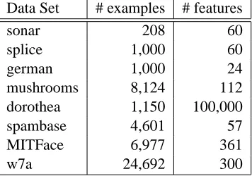
(g) MITFace (h) w7a

Algorithm vehicle dna

Mistake (%) Support Vectors (#) Time (s) Mistakes (%) Support Vectors (#) Time (s)

Max 64.882±1.643 548.90±13.90 0.079 20.460±0.770 409.20±15.41 0.192

Uniform 65.934±1.554 557.80±13.15 0.109 19.875±0.427 397.50±8.54 0.264 Prop 66.678±1.757 564.10±14.86 0.116 20.268±0.555 405.35±11.10 0.267 MIRA 62.252±2.114 526.65±17.89 1.821 26.920±0.880 538.40±17.61 5.304 PA-I 67.086±1.479 781.70±12.42 0.091 15.503±0.474 1224.35±13.48 0.326 PA-II 66.909±1.475 789.30±10.73 0.089 15.398±0.467 1237.50±13.12 0.325 M-DUOLiter 70.674±1.194 758.05±8.65 0.162 11.668±0.599 1086.00±16.39 0.502

M-DUOLappr 69.634±1.463 828.05±4.48 0.158 14.105±0.611 1281.75±14.44 0.495 M-DUOL 51.950±1.948 719.25±10.95 0.172 10.340±0.513 869.80±12.61 0.438

Algorithm segment satimage

Mistake (%) Support Vectors (#) Time (s) Mistakes (%) Support Vectors (#) Time (s)

Max 41.342±1.013 955.00±23.40 0.414 29.628±0.561 1314.00±24.89 0.826

Uniform 41.468±0.550 957.90±12.71 0.566 28.440±0.398 1261.30±17.64 1.071 Prop 41.589±0.714 960.70±16.48 0.565 28.878±0.467 1280.75±20.72 1.087 MIRA 35.784±3.770 826.55±87.08 9.193 27.536±2.228 1221.20±98.80 15.229 PA-I 39.775±0.665 1852.75±19.90 0.573 27.377±0.361 2676.40±24.88 1.296 PA-II 39.842±0.655 1870.70±18.97 0.577 27.258±0.429 2709.50±23.77 1.307 M-DUOLiter 41.416±1.084 1787.90±31.00 0.903 33.894±0.567 2787.45±43.18 2.024 M-DUOLappr 39.314±0.791 1923.60±14.31 0.871 26.222±0.464 3052.50±31.39 2.024 M-DUOL 20.580±0.705 1265.15±28.39 0.693 22.524±0.482 2066.85±32.99 1.505

Algorithm usps mnist

Mistake (%) Support Vectors (#) Time (s) Mistakes (%) Support Vectors (#) Time (s)

Max 10.025±0.195 730.90±14.21 1.459 15.318±0.168 1531.80±16.80 2.744

Uniform 9.445±0.150 688.60±10.91 1.858 14.603±0.201 1460.25±20.15 3.631 Prop 9.614±0.176 700.95±12.86 1.868 14.763±0.228 1476.30±22.78 3.635 MIRA 11.572±0.403 843.75±29.39 44.663 18.037±0.539 1803.70±53.93 67.168 PA-I 6.641±0.158 2528.45±23.48 2.669 11.026±0.208 4773.70±32.84 5.771 PA-II 6.568±0.116 2561.95±27.94 2.606 10.959±0.238 4830.40±27.06 5.824 M-DUOLiter 5.743±0.158 2284.15±40.06 3.160 8.947±0.182 4398.95±46.46 9.031 M-DUOLappr 6.002±0.132 2725.40±23.55 3.541 9.640±0.164 5163.05±37.34 10.386

M-DUOL 5.162±0.149 1759.30±23.44 2.408 8.282±0.183 3557.15±25.17 7.050

Algorithm letter protein

Mistake (%) Support Vectors (#) Time (s) Mistakes (%) Support Vectors (#) Time (s)

Max 71.562±0.538 10734.35±80.63 18.749 47.657±0.221 8466.75±39.21 12.842

Uniform 71.973±0.280 10795.90±41.99 47.031 46.828±0.272 8319.45±48.36 14.342 Prop 72.033±0.273 10804.95±40.89 43.683 47.260±0.260 8396.15±46.13 14.620 MIRA 67.709±1.196 10156.35±179.54 467.019 47.905±0.922 8510.80±163.74 42.174 PA-I 72.283±0.338 14708.55±15.27 24.848 47.657±0.230 14153.25±49.06 23.409 PA-II 72.339±0.380 14735.55±15.86 24.131 47.550±0.285 14285.85±44.94 23.602 M-DUOLiter 73.066±0.326 14614.65±22.26 210.684 50.070±0.392 14191.85±64.80 55.622

M-DUOLappr 69.992±0.331 14892.70±11.77 215.587 51.459±0.582 16000.55±72.07 63.065 M-DUOL 54.068±0.351 13140.40±37.33 186.452 46.281±0.418 12550.10±87.27 43.774

Prop) and MIRA are considerably sparser than those learned by the two PA algorithms. We believe that this can be attributed to the aggressive updating strategies used by the PA algorithms. Second, among the three variants of double updating for multi-label learning, it is not surprising to observe that M-DUOL yields the lowest mistake rates for all data sets. Further, among all the algorithms, we observe that the M-DUOL algorithm makes the least number of mistakes for all data sets, and significantly outperforms all the baseline algorithms.

Second, by examining the sparsity of classifiers learned by the proposed algorithms, we observe that the number of support vectors identified by M-DUOL is usually smaller than that of the PA algorithms (except for data set “vehicle”), but is significantly larger than those of the four non-aggressive algorithms (i.e., Max, Uniform, Prop, and MIRA).

Finally, comparing the running time cost, we observe that the Max algorithm is the most effi-cient one, while MIRA is the least effieffi-cient approach for all the data sets. Despite the additional time needed for double updates, overall we found that the running time of the proposed M-DUOL algorithm is comparable to those of the two PA algorithms (except for the “letter” data set where the time costs of the M-DUOL algorithms are considerably greater than those of the PA algorithms).

6. Discussions and Future Directions

Although encouraging results have been achieved by the proposed novel DUOL algorithms, we should address the limitations of our current work and discuss some research directions for future improvements. First of all, the proposed DUOL algorithm is based on the Passive Aggressive on-line learning algorithms (Crammer et al., 2006). For the future work, it is possible to extend other single update online learning methods, such as EG (Kivinen and Warmuth, 1995), for double up-dating. Second, the approach for choosing an auxiliary example from existing support vectors may be further improved by exploring the heuristics for measuring the informativeness of an example. Finally, we plan to extend the proposed double updating framework for budget online learning to make sparse classifiers.

7. Conclusions

This paper presented a novel “double updating” approach to online learning named as “DUOL”, which not only updates the weight of the misclassified example, but also adjusts the weight of one existing support vector that the most seriously conflicts with the new support vector. We show that the mistake bound for an online classification task can be significantly reduced by the proposed DUOL algorithms. We have conducted an extensive set of experiments by comparing with a number of algorithms for both binary and multiclass online classifications. Promising empirical results showed that the proposed double updating online learning algorithms consistently outperform the single-update online learning algorithms.

Acknowledgments

Appendix A. The Proof for Proposition 2

Proof The optimization (1) can be rewritten to the following equivalent optimization:

min

γa,dγb

ka

2γ

2 a+

kb

2d

2

γb+wabγadγb−ℓaγa−ℓbdγb,

s.t. γa−C≤0, (6)

−γa≤0, (7)

dγb−C+γˆb≤0, (8)

−dγb−γˆb≤0, (9)

where ka,kb>0, wab≤0, ℓa=1−yaf(xa)≥0, ℓb=1−ybf(xb)≥0 and ˆγb>0. With λ1, λ2,

λ3 andλ4 as Lagrange multipliers, the KKT conditions for this problem consist of the constraints

(6)-(9), the nonnegativity constraintsλi≥0, ∀i, the complementary slackness conditions

λ1(γa−C) =0, λ2(−γa) =0,λ3(dγb−C+γˆb) =0,λ4(−dγb−ˆγb) =0

and zero gradient conditions:

kaγa+wabdγb−ℓa+λ1−λ2=0 and kbdγb+wabγa−ℓb+λ3−λ4=0.

We will discuss every possible condition to compute the closed-form solution. Firstly, we will dis-cuss the caseλ16=0:

A.1 Case 1. Ifλ16=0

Sinceλ1(γa−C) =0, we haveγa=C; further, becauseλ2(−γa) =0, we haveλ2=0. Under the

conditionλ16=0, we will discussλ36=0 andλ3=0 separately as follows:

A.1.1 SUB-CASE1.1. IFλ36=0

Sinceλ3[dγb−(C−ˆγb)] =0, we have dγb=C−γˆb, as a resultλ4(−C) =0, soλ4=0. Plugging the

resultsγa=C,λ2=0, dγb =C−ˆγbandλ4=0 into the zero gradient condition, we have

kaC+wab(C−γˆb)−ℓa+λ1=0 and kb(C−γˆb) +wabC−ℓb+λ3=0.

Thus, we have

λ1=−[kaC+wab(C−ˆγb)−ℓa] and λ3=−[kb(C−γˆb) +wabC−ℓb].

As a result, if

−(kaC+wab(C−γˆb)−ℓa)>0 and −(kb(C−γˆb) +wabC−ℓb)>0,

A.1.2 SUB-CASE1.2. IFλ3=0

Whenλ3=0, we only conclude dγb∈[−γˆb,C−ˆγb].

Under the conditionsλ16=0 andλ3=0, we will discuss the two casesλ46=0 andλ4=0,

respec-tively as follows.

Sub-case 1.2.1. Ifλ46=0. Sinceλ4(−dγb−γˆb) =0, we have dγb=−γˆb. Plugging the resultsλ2=0,

γa=C,λ3=0 and dγb=−ˆγbin to the zero gradient conditions:

kaC+wab(−γˆb)−ℓa+λ1=0 and kb(−γˆb) +wabC−ℓb−λ4=0.

But since kb(−γˆb)<0 wabC≤0 andℓb,λ4≥0, kb(−ˆγb) +wabC−ℓb−λ4<0, which contradicts

the equation above.

Sub-case 1.2.2. Ifλ4=0. Plugging the conditionsγa=C,λ2=0,λ3=0 andλ4=0 into the zero

gradient equations:

kaC+wabdγb−ℓa+λ1=0 and kbdγb+wabC−ℓb=0.

Solving the above equations leads to the following:

λ1=

w2_abC−wabℓb−kakbC+kbℓa kb

and d_γb =

ℓb−wabC

kb

.

Ifw2abC−wabℓb−kakbC+kbℓa

kb >0 and

ℓb−wabC

kb ∈[−ˆγb,C−ˆγb], then the KKT conditions are all satisfied; as

a result,(γa,dγb) = (C, ℓb−wabC

kb )is the unique optimal solution.

Next we will discuss the situation with the conditionλ1=0.

A.2 Case 2. Ifλ1=0

Under the conditionλ1=0, we only conclude γa∈[0,C]. We will discuss the cases λ26=0 and

λ2=0 under the conditionλ1=0, respectively.

A.2.1 SUB-CASE2.1. IFλ₂6=0

Sinceλ2(−γa) =0, we concludeγa=0. Under the conditionsλ1=0 andλ26=0, we will discuss

the casesλ36=0 andλ3=0:

Sub-case 2.1.1. If λ36=0. Sinceλ3[dγb−(C−γˆb)] =0, plugging the conditions λ1=0, γa=0,

dγb =C−ˆγbandλ4=0 into the zero gradient conditions:

wab(C−ˆγb)−ℓa−λ2=0 and kb(C−ˆγb)−ℓb+λ3=0.

Since wab≤0, C−γˆb≥0 andℓa≥0, we conclude

λ2=wab(C−γˆb)−ℓa≤0.

Butλ2≥0 andλ26=0, concludeλ2>0, which contradicts the inequality above.

Sub-case 2.1.2. Ifλ3=0. Under these known conditions, we only know dγb ∈[−γˆb,C−ˆγb]. Below,