Exploiting Best-Match Equations for Efficient Reinforcement Learning

(1)

Exploiting Best-Match Equations

for Efficient Reinforcement Learning

Harm van Seijen [email protected]

Distributed Sensor Systems Group TNO Defence, Security and Safety P.O. Box 96864

2509 JG, The Hague, The Netherlands

Shimon Whiteson [email protected]

Informatics Institute University of Amsterdam Amsterdam, The Netherlands

Hado van Hasselt [email protected]

Multi-agent and Adaptive Computation Group Centrum Wiskunde & Informatica

Amsterdam, The Netherlands

Marco Wiering [email protected]

Department of Artificial Intelligence University of Groningen

Groningen, The Netherlands

Editor: Peter Dayan

Abstract

This article presents and evaluates best-match learning, a new approach to reinforcement learning that trades off the sample efficiency of based methods with the space efficiency of model-free methods. Best-match learning works by approximating the solution to a set of best-match

equations, which combine a sparse model with a model-free Q-value function constructed from

samples not used by the model. We prove that, unlike regular sparse model-based methods, best-match learning is guaranteed to converge to the optimal Q-values in the tabular case. Empirical results demonstrate that best-match learning can substantially outperform regular sparse model-based methods, as well as several model-free methods that strive to improve the sample efficiency of temporal-difference methods. In addition, we demonstrate that best-match learning can be suc-cessfully combined with function approximation.

Keywords: reinforcement learning, on-line learning, temporal-difference methods, function ap-proximation, data reuse

1. Introduction

(2)

expected return, which is the cumulative discounted reward. When the sequential decision problem is modeled as a Markov decision process (MDP), the agent’s policy can be represented as a mapping from each state it may encounter to a probability distribution over the available actions.

There are several approaches for learning the optimal policy of an MDP. Model-free, or di-rect, methods find an optimal policy by using sample experience to directly update the state values, which predict the return when following a specified policy, or the state-action values, or Q-values, which predict the return when taking an action in a certain state and following a specified policy thereafter. Once the optimal state or state-action values have been found, the optimal policy can easily be constructed. A popular model-free approach is temporal-difference (TD) learning (Sut-ton, 1988), which bootstraps value estimates from other values using updates based on the Bellman equations (Bellman, 1957). Temporal-difference methods such as Q-learning (Watkins, 1989) and Sarsa (Rummery and Niranjan, 1994; Sutton, 1996) require only

O

(|

S

||

A

|) space and are guaran-teed to find optimal policies in the limit. However, they often need prohibitively many samples in practice.

Alternatively, model-based, or indirect, methods (Sutton, 1990; Moore and Atkeson, 1993; Braf-man and Tennenholtz, 2002; Kearns and Singh, 2002; Strehl and LittBraf-man, 2005; Diuk et al., 2009) use sample experience to estimate a model of the MDP and then compute the optimal values us-ing this model via off-line plannus-ing techniques such as dynamic programmus-ing (Bellman, 1957). Because the sample experience gathered by the agent is incorporated into the model, it is reused throughout learning. As a result, some model-based methods can find approximately optimal poli-cies with high probability using only a polynomial number of samples (Brafman and Tennenholtz, 2002; Kearns and Singh, 2002; Strehl and Littman, 2005). However, representing the model requires

O

(|

S

|2_|

_A

_|₎_{space, which can be prohibitive in problems with large state spaces.}

To avoid this limitation, methods can learn smaller, approximate models that require only a frac-tion of the space used by full model-based methods. Kearns and Singh (1999) show that, when using such sparse models, it is still possible to learn probably approximately correct policies. However, the performance of such methods is bounded by the quality of the model approximation. Furthermore, since the models may remain incorrect regardless of how much sample experience is gathered, such methods are not guaranteed to find optimal policies even in the limit.

In this article, we present and evaluate best-match learning, a new approach for trading off the strengths of model-based and model-free methods. Best-match learning works by approximating the solution to a set of best-match equations, which combine a sparse model with a model-free Q-value function constructed from samples not used by the model. We prove that, unlike regular sparse model-based methods, best-match learning is guaranteed to converge to the optimal policy in the tabular case. This guarantee holds even when using a last-visit model (LVM), which stores only the last observed reward and transition state for each state-action pair.

(3)

The rest of this article is organized as follows. Section 2 formally defines the RL problem and summarizes some basic theoretical results. As a conceptual stepping stone, Section 3 presents just-in-time Q-learning, which postpones updates until the moment of revisit of the corresponding state. We prove that, although just-in-time Q-learning performs the same number of updates as regular Q-learning, the Q-values used in its update targets generally have received more updates. Thus, it can improve performance without extra computation.

Section 4 extends the idea of using improved update targets to best-match learning with an LVM, in which updates are continually revised such that the update targets constructed from them are more accurate. We show that best-match LVM learning is related to eligibility traces, by proving that under certain conditions they compute the same values. However, we also show that in arbitrary MDPs best-match LVM learning, unlike eligibility traces, performs updates that are unbiased with respect to initial state values. We demonstrate empirically that, as a result, it can substantially outperform TD(λ) despite using similar space and computation.

Section 4 also addresses the control case. We propose an efficient best-match LVM algorithm that uses prioritized sweeping (Moore and Atkeson, 1993), a well-known technique for prioritizing model-based updates, to trade off extra computation for improved performance. We prove that, despite the use of a sparse model, this approach converges to the optimal Q-values under the same conditions as Q-learning. In addition, we demonstrate empirically that it can substantially outper-form competitors with similar space requirements.

Section 5 proposes a best-match learning algorithm that uses an n-transition model (NTM), which maintains an estimate of the transition probability for n transition states per state action pair. By tuning n, the space requirements can be controlled. We prove that the algorithm converges to the optimal Q-values for any value of n. We demonstrate empirically the resulting performance improvement over regular sparse model-based methods with equal space requirements, whose per-formance is bounded by the quality of the model approximation.

Section 6 proposes best-match function approximation, which demonstrates that best-match learning is useful beyond the tabular case. In particular, we combine best-match learning with gradient-descent function approximation and show empirically that it can outperform Sarsa(λ) and experience replay with linear function approximation while using similar computation.

Section 7 discusses the article’s theoretical and empirical results, Section 8 outlines future work, and Section 9 concludes.

2. Background

Sequential decision problems are often formalized as Markov decision processes (MDPs), which can be described as 4-tuples h

S

,

A

,

P

,

R

i consisting of

S

, the set of all states;

A

, the set of all actions;

P

s′

sa=P(s′|s,a), the transition probability from state s∈

S

to state s′ when action a∈

A

is

taken; and

R

_sa=E(r|s,a), the reward function giving the expected reward r when action a is taken in state s. Actions are selected at discrete timesteps t=0,1,2, ...and rt+1is defined as the reward received after taking action atin state st at timestep t. An optimal policyπ∗is a mapping from

S

to

A

that maximizes the expected discounted return

Rt=rt+1+γrt+2+γ2rt+3+...=

∞

∑

k=0 γk_r

(4)

Most solution methods are based on estimating a value function Vπ(s), which gives the expected return when the agent is in state s and follows policyπ, or an action-value function Qπ(s,a), which gives the expected return when the agent takes action a in state s and follows policyπthereafter.

In the control case, TD methods seek to learn the optimal action-value function Q∗(s,a), which is the solution to the Bellman optimality equations (Bellman, 1957):

Q∗(s,a) =

R

_sa+γ

∑

s′

P

s′ samax

a′ Q

∗₍_s′_,_a′₎_.

By iteratively updating the current estimate Qt(s,a) each time new experience is obtained, TD

methods seek to approximate this function. A common form for these updates is

Qt+1(st,at)←(1−α)Qt(st,at) +αυt,

whereαis the learning rate andυt is the update target. Many update targets are possible, such as

the Q-learning (Watkins and Dayan, 1992) update target

υt=rt+1+γmax

a Qt(st+1,a).

Once the optimal action-value function has been learned, an optimal policy can be derived by taking the greedy action with respect to this function.

Alternatively, the agent can take a model-based approach (Sutton, 1990; Moore and Atkeson, 1993), in which its experience is used to compute maximum-likelihood estimates of

P

and

R

. Using this model, the agent can compute Q (or the value function V ) using dynamic programming methods (Bellman, 1957) such as value iteration (Puterman and Shin, 1978). Each time new experience is gathered, the model is updated and Q recomputed.

In the control case, the agent faces the exploration-exploitation dilemma. The agent can either exploit its current knowledge by taking the action that predicts the highest expected return given current estimates, or it can explore by taking a different action in order to improve the accuracy of the Q-value of that action.

Related to the control case is the policy evaluation case. In this case, the goal is to estimate the value function Vπ(s)belonging to policyπ. TD methods iteratively improve the current estimate, Vt(s)each time new experience is obtained using the update rule

Vt+1(st)←(1−α)Vt(st) +αυt.

An example of an update target for policy evaluation is the TD(0) update target

υt=rt+1+γVt(st+1).

3. Just-In-Time Q-Learning

(5)

more updates, while the total number of updates of the current state stays the same. Empirically, we demonstrate that this leads to a performance gain under a range of settings at similar computational cost.

When a Q-learning update is postponed, the values on which the update target is based are from a more recent timestep. This is advantageous, since Q-learning updates cause the expected error in the values to decrease over time (Watkins and Dayan, 1992) and therefore more recent values will be on average more accurate. However, postponing the update of a value for too long can negatively affect performance, since a value that has not been updated might be used for action selection or for bootstrapping other values. We start by showing that updates can be postponed until their corresponding states are revisited, without negatively affecting performance.

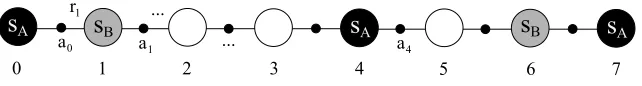
Figure 1: A state transition sequence in which the initial state sA is revisited at timestep 4. The

small black dots in between states represent actions.

Consider the state-action sequence in Figure 1. State sA is visited at timestep 0 and revisited at

timestep 4. With the regular Q-learning update, the Q-value of state-action pair(sA,a0)gets updated

at timestep 1:

Q1(sA,a0) = (1−α)Q0(sA,a0) +α[r1+γmax

a Q0(sB,a)],

while at timesteps 2−4 no update of(sA,a0) occurs, and therefore Q4(sA,a0) =Q1(sA,a0). The update of the Q-value of(sA,a0)at timestep 1 can be considered premature, since the earliest use

of its value is in the update target for(sD,a3), which uses Q3(sA,a0). Therefore, the update of the Q-value of(sA,a0)can be postponed until at least timestep 3 without negatively affecting the update target for(sD,a3). When the update of(sD,a3)is also postponed, the earliest use of the Q-value of (sA,a0)occurs at timestep 4, where it is used for action selection. Thus, if we postpone the update of all state-action pairs, the update of the Q-value of(sA,a0)can be postponed until the timestep of its revisit, without causing dependent state values or the action selection procedure to use a value of

(sA,a0)that has not been updated. We call this type of update a just-in-time update, since the update is postponed until just before the updated value is needed.

To denote the Q-values resulting from just-in-time updates we use ˜Q throughout this section. With just-in-time updates, no updates of(sA,a0)occur at timesteps 1-3, so ˜Q3(sA,a0) =Q0˜ (sA,a0).

Instead, an update occurs when sA is revisited:

˜

Q4(sA,a0) = (1−α)Q˜3(sA,a0) +α[r1+γmax

a

˜

Q3(sB,a)].

The regular and just-in-time update for(sA,a0)can be written in a more similar form by expressing the value at timestep 4 in terms of the value at timestep 0:

Q4(sA,a0) = (1−α)Q0(sA,a0) +α[r1+γmax

a Q0(sB,a)],

˜

Q4(sA,a0) = (1−α)Q0˜ (sA,a0) +α[r1+γmax a

˜

(6)

This formulation highlights the difference between the two update types. At timestep 4, under both update schemes, the Q-value of(sA,a0)has received one update based on the same experience

sample. However, a just-in-time update uses the most recent value of the Q-values of sB, while a

regular update uses the value at the timestep of the initial visit of sA. By defining t∗as the timestep

of the previous visit of state st, we can write the two update types more generally as

Qt(st,at∗) = (1−α)Q_t∗(s_t,a_t∗) +α[r_t∗₊₁+γmax

a Qt∗(st∗+1,a)], (2)

˜

Qt(st,at∗) = (1−α)Q˜t∗(st,at∗) +α[rt∗+1+γmax

a

˜

Qt−1(st∗+1,a)]. (3) Note that we express the update target using only values from the past, making an implementation easier to interpret. Note also that while st=st∗per definition (because s_tis revisited), s_t∗₊₁does not

have to be equal to st+1, since the state transition from st can be stochastic. Also, at∗ is in general

not equal to at.

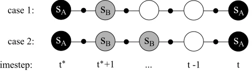
When comparing the two update targets in more detail, two cases can be distinguished. See Figure 2 for an example of each case. In the first case, state sBis not revisited before the revisit of

state sA. In this case, neither update type makes use of an updated Q-value for sBin the update target

for sA. The regular update does not since it uses the values of sBat timestep t∗, and the just-in-time

update does not since sBis not revisited and therefore no update has occurred yet at timestep t−1.

In the second case, state sBhas been revisited before the revisit of sA. The regular update still uses

the value of sBfrom timestep t∗and therefore does not use an updated value. The just-in-time update

on the other hand does use an updated value, since this update occurred at the revisit of sB. Note

that for a returning action (t∗=t−1), both update types have exactly the same form and this can therefore be treated as an example of case 1. From these two cases, we can deduce the following theorem, which is proven in Appendix A.

Theorem 1 Given the same experience sequence, each Q-value from the current state has received the same number of updates using JIT updates (Equation 3) as using regular updates (Equation 2). However, each Q-value in the update target of a JIT update has received an equal or greater number of updates as in the update target of the corresponding regular update.

Figure 2: Two cases in which state sA is revisited. In the first case, neither a regular update nor a

just-in-time update make use of an updated value for sBin the update target of sA, while

in the second case a just-in-time update does.

(7)

Algorithm 1 JIT Q-Learning

1: initialize Q(s,a)arbitrarily for all s,a

2: initialize S′(s) =/0for all s

3: loop{over episodes}

4: initialize s

5: repeat{for each step in the episode}

6: if S′(s)6=/0then

7: Q(s,a¯)←(1−αs ¯a₎_·_Q₍_s_,_a_¯_{) +}_αs ¯a_[_R′₍_s_{) +}_γ_max

a′ Q(S′(s),a′)] //a¯=A(s) 8: end if

9: select action a, based on Q(s,·) 10: take action a, observe r and s′

11: S′(s)←s′; R′(s)←r; A(s)←a

12: s←s′

13: until s is terminal

14: end loop

in A(s). If S′(s) =/0, state s has not been visited yet and no update can be performed. Note that the last-visit sample is not reset at the end of an episode, but maintained across episodes.

Because JIT Q-learning uses more recent values in its update targets than regular Q-learning, we expect a performance improvement over regular Q-learning. We test this hypothesis by comparing the performance of JIT Q-learning with regular Q-learning on the Dyna Maze task (Sutton, 1990). In this navigation task, depicted in Figure 3, the agent has to find its way from start to goal. The agent can choose between four movement actions: up, down, left and right. All actions result in 0 reward, except for when the goal is reached, which results in a reward of +1. The discount factor

γis set to 0.95. We use a deterministic as well as a stochastic environment to test the generality of the hypothesis. In the stochastic version, we employ a probabilistic transition function: with a 20% probability, the agent moves in an arbitrary direction instead of the direction corresponding to the action.

To compare performance, we measure the average return each method accrues from the start state during the first 100 episodes in the deterministic case, averaged over 5000 independent runs per method. For the stochastic version, we measure the return during the first 200 episodes. Each method usesε-greedy action selection with ε=0.1. In the deterministic case, we use a constant learning rate of 1, while in the stochastic case we use an initial learning rateα0of 1 that is decayed in the following manner:1

αsa₌ α0

d·[n(s,a)−1] +1, (4)

where n(s,a)is the total number of times action a has been selected in state s. Note that for d=0,

αsa₌_α

0, while for d=1,αsa=α0/n(s,a). We optimize the learning rate decay d between 0 and 1 by taking the decay rate with the maximum average return over the measured number of episodes. We use two different initialization schemes for the Q-values to determine whether the performance difference depends on initialization. We use optimistic initialization, by initializing the Q-values to 20, and pessimistic initialization, by setting the Q-values to 0.

1. This decay is similar to the more common form c1

(8)

S

G

Figure 3: The Dyna Maze task, in which the agent must travel from S to G. The reward is +1 when the goal state is reached and 0 otherwise.

0 20 40 60 80 100 0

0.05 0.1 0.15 0.2 0.25 0.3 0.35 0.4 0.45 0.5

episodes

return

0 50 100 150 200

0 0.05 0.1 0.15 0.2 0.25 0.3 0.35 0.4

episodes

return

JIT Q−learning, Q 0 = 20 Q−learning, Q

0 = 20 JIT Q−learning, Q

0 = 0 Q−learning, Q

0 = 0

Figure 4: Comparison of the performance of JIT Q-learning and regular Q-learning on the de-terministic (left) and stochastic (right) Dyna Maze task for two different initialization schemes.

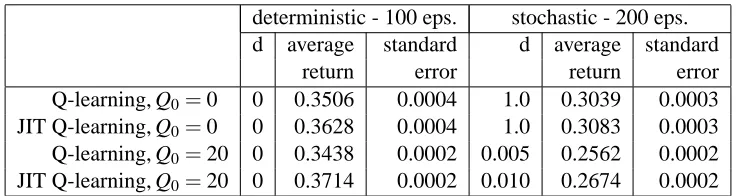
deterministic - 100 eps. stochastic - 200 eps. d average standard d average standard

return error return error

Q-learning, Q0=0 0 0.3506 0.0004 1.0 0.3039 0.0003 JIT Q-learning, Q0=0 0 0.3628 0.0004 1.0 0.3083 0.0003 Q-learning, Q0=20 0 0.3438 0.0002 0.005 0.2562 0.0002 JIT Q-learning, Q0=20 0 0.3714 0.0002 0.010 0.2674 0.0002

Table 1: The performance of JIT Q-learning and regular Q-learning on the Dyna Maze task and the optimal learning rate decay d.

(9)

environ-ment and for both types of initialization, although not always by a large margin. This confirms our intuition that, since JIT Q-learning uses values from a later time which are in general more accurate, a performance benefit is gained over regular Q-learning in a broad range of settings. The perfor-mance benefit in the deterministic case can be explained by exploration, which causes the order in which states are visited to change despite the deterministic state transitions.

4. Best-Match Last-Visit Model

In this section, we demonstrate that updates can be postponed much further than is done by JIT Q-learning, without negatively affecting other updates, when best-match updates are performed. Best-match updates are updates that can correct previous updates when more recent information becomes available. This insight leads to the derivation of the best-match last-visit model equations, which combine a last-visit model (LVM), consisting of the last experienced reward and transition state for each state-action pair, with model-free Q-values, constructed from model-free updates of all observed samples, except the ones stored in the LVM. We present an evaluation as well as a control algorithm based on solving these equations and empirically demonstrate that these methods can outperform competitors with similar space requirements.

4.1 Best-Match LVM Equations

In the example presented in Section 3, the update of Q(sA,a0)is postponed until state sAis revisited.

In this section, we demonstrate that the update can be postponed even further in the case that a different action is selected upon revisit. Since we will consider multiple updates per timestep in this section, we denote the Q-value function using two iteration indices: t and i. Each time an update occurs, i is increased, while each time an action is taken, t is increased and i is reset to 0. Therefore, if I denotes the total number of updates that occurs at time t, by definition Qt,I=Qt+1,0. Action selection at time t is based on Qt,I. Using this convention, the regular Q-learning update can be

written as

Qt+1,1(st,at) = (1−α)Qt+1,0(st,at) +α[rt+1+max

a′ Qt+1,0(st+1,a

′_)]_.

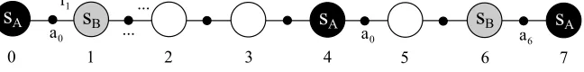
Now consider the example shown in Figure 5, which extends Figure 1 to include a second revisit of s0at timestep t=7. Suppose that a different action is selected on the first revisit, that is, a46=a0. Using just-in-time updates, the Q-value of state-action pair(sA,a0)gets updated at time t=4. Using the two indices convention we can rewrite Equation 1 as2

Q4,1(sA,a0) = (1−α)Q1,0(sA,a0) +α[r1+γmax

a Q4,0(sB,a)]. (5)

To perform this update, the experience set(r1,sB)resulting from taking action a0in sA is

tem-porarily stored. With JIT Q-learning, this experience is stored per state. If the state is revisited and a new action is taken, the previous experience is overwritten and lost. However, if the experience is stored per state-action pair, then the previous experience is not overwritten until the same action is selected again. If the same action is not selected upon revisit, the experience can be used again

2. We use Q now instead of ˜Q, since the only purpose of the tilde was to distinguish it from the Q-values of regular

(10)

Figure 5: A state transition sequence in which best-match updates can enable further postponing. Timesteps are shown below each state.

to redo the update at a later time, using more recent values for the next state. In the example from Figure 5, the update of(sA,a0)can be redone at timestep 7:

Q7,1(sA,a0) = (1−α)Q1,0(sA,a0) +α[r1+γmax

a Q7,0(sB,a)]. (6)

Since state sBis revisited at timestep 6,(sB,a1)has received an extra update and therefore Q7,0(sB,a1) is likely to be more accurate than Q4,0(sB,a1).

Equation 6 is not equivalent to a (postponed) Q-learning update, in contrast to Equation 5, since Q1,0(sA,a0) is not equal to Q7,0(sA,a0) due to the update at timestep 4. Equation 6 corrects the

update from timestep 4, by redoing it using the most recent Q-values for the update target. We call this update a best-match update (this name will be explained later in the section), while we call Q1,0(sA,a0)the model-free Q-value of(sA,a0).

Before formally defining a best-match update, we define the last-visit experience and the model-free Q-values.

Definition 2 The last-visit experience of state-action pair(s,a)denotes the last-visit reward, R′_t(s,a), that is, the reward received upon the last visit of(s,a), and the last-visit transition state, S′_t(s,a), that is, the state transitioned to upon the last visit of(s,a). For a state-action pair that has not yet been visited, we define R′_t(s,a) =/0and S′_t(s,a) =/0.

The LVM consists of the last-visit experience from all state-action pairs.

Definition 3 The model-free Q-value of a state-action pair(s,a), Q_tm f(s,a), is a Q-value that has received updates from all observed samples except those stored in the LVM, that is, R′_t(s,a)and S′_t(s,a). For a state-action pair that has not yet been visited, we define Qtm f(s,a) =Q0,0(s,a). While Q can be updated multiple times per timestep, Qm f is updated only once per timestep. There-fore, it is uses a single time index t. We define a best-match update as:

Definition 4 A best-match update combines the model-free Q-value of a state-action pair with its last-visit experience from the same timestep according to

Qt,i+1(s,a) = (1−α)Qtm f(s,a) +α[R′t(s,a) +γmax a′ Qt,i(S

′

t(s,a),a′)].

Using best-match updates to extend the postponing period of a sample update requires addi-tional computation, as the agent typically performs multiple best-match updates per timestep. In the example, at timestep 7 the agent redoes the update of Q(sA,a0), but also performs an update of

(11)

The model-free Q-value function is updated only once per timestep. Specifically, at timestep t+1 Qm f is updated according to

Qm f_t₊₁(st,at) =Qt+1,0(st,at). (7)

Assuming (st,at) has received a best-match update at timestep t, Equation 7 is equivalent to the

update

Q_tm f₊₁(st,at) = (1−α)Qtm f(st,at) +α[R′t(st,at) +γmax a′ Qt,i(S

′

t(st,at),a′)],

where the value of i depends on the order of best-match updates at timestep t. After Qm f _{has been}

updated, the last-visit experience for(st,at)is overwritten with the new experience

R′_t₊₁(st,at) = rt+1, S′_t₊₁(st,at) = st+1.

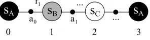
In the approach described above, best-match updates are used to postpone the update from a sample without negatively affecting other updates or the action selection process. However, best-match updates can be exploited far beyond simply avoiding these negative effects. As an example, consider the state-action sequence in Figure 6. sBis not revisited before the revisit of sA. With the

update strategy described above, best-match updates occur only when a state is revisited. Conse-quently, the experience from(sB,a1)is not used in the update target of(sA,a0). However, it is not

necessary to wait for a revisit of sBto perform a best-match update. Instead, it can be performed at

the moment it is needed: when sAis revisited. Thus, if at timestep 3 the agent performs a best-match

update of Q(sB,a1), before updating Q(sA,s0), the latter update will exploit more recent Q-values

for sB, just as if sBhad been revisited.

Figure 6: A state transition sequence in which sBis not revisited. Timesteps are shown below each

state.

Taking this idea further, the agent can first update the Q-values of sC before updating the

Q-values of sB. In other words, the agent uses the Q-values of sA to perform a best-match update of

sC, then performs a best-match update of sB and finally updates sA. However, once the Q-values

of sAhave changed, it is possible to further improve the Q-values of sC by performing a new

best-match update. The new Q-values of sC can then be used to redo the update of sB, which in turn can

be used to re-update sA. This process can repeat until the Q-values reach a fixed point, which is

the solution to a system of|

S

||

A

|best-match LVM equations. We call this solution the best-match Q-value function, QB, which forms the best match between the LVM and the model-free Q-values.

Definition 5 The best-match LVM equations at timestep t are defined as

Q_tB(s,a) = (

(1−αsa t )Q

m f

t (s,a) +αsat [R′t(s,a) +γmaxcQtB(S′t(s,a),c)] if S′t(s,a)6= /0

(12)

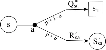
There are different ways to look at these equations. One way is to see them as the limit case of redoing updates using (in general) increasingly more accurate update targets. Another way is to see them as Bellman optimality equations based on an induced model. For state-action pair(s,a)this induced model can be described as a transition with probabilityαto state S′(s,a)with a reward of R′(s,a)and a transition with probability 1−αto a terminal state sT (with a value of 0) and a reward

of Qm f(s,a)(see Figure 7).3

S´

R´

s

a

s

T

sa sa

Q

sa

mf

p = α p =

α

Figure 7: Illustration of the induced model for state-action pair(s,a)corresponding with the best-match LVM equations. The small black dot represents the stochastic action a leading with probabilityαto state S′(s,a)and with probability 1-αto state sT.

The advantage of solving the Bellman optimality equations for this induced model, compared to solving it using only the LVM, is that the bias towards the samples in the LVM can be controlled using the learning rates. With annealing learning rates, the transition probability to S′_t(s,a)is de-creased over time in favor of transition to the terminal state. On the other hand, when using only the LVM, the solution of the Bellman equations depends only on the samples of the LVM and does not take into account any previous samples. Clearly, in a stochastic environment, this will lead to a sub-optimal policy. Also when the solution is not computed exactly, but approximated by only per-forming a finite number of updates at each timestep (which is the case for any practical algorithm), using the induced model leads to a better performance, because of the strong bias towards the most recent samples that occurs when using only the LVM.

Section 4.3 discusses how to solve the best-match equations. However, we first discuss the policy evaluation case, for which analogous equations can be defined.

Definition 6 The best-match LVM equations for state values at time t are

V_tB(s) = (

(1−αs t)V

m f

t (s) +αst[R′t(s) +γVtB(S′t(s))] if S′t(s)6=/0

V_tm f(s) if S′_t(s) =/0.

The model-free state values are updated according to V_tm f₊₁(st) =Vt+1,0(st).

While in general the value function V can be seen as a special case of the action-value function Q (with all states only having a single action), V has a linear set of best-match equations, in contrast to Q, a property we exploit in best-match LVM evaluation.

(13)

4.2 Best-Match LVM Evaluation

In the evaluation case, the best-match LVM equations form a linear set that can be solved exactly. This section proposes an algorithm that does so in a computationally efficient way, using updates that are unbiased with respect to the initial state values.

The algorithm is based on two observations. First, not all|

S

|best-match equations necessarily depend on each other. The subset of equations needed to compute the best-match value for st can

be found by iterating through the sequence of last-visit transition states, starting with S′(st). The

corresponding N best-match equations form the linear set of equations to solve. For readability, we write stas s[0]and use the notation s[n]=S′(s[n−1])and r[n]=R′(s[n−1])for the subsequent transition state and reward. In addition, we useα[n] forαs[n]_{. The equations can now be written as}

VB(s_[_n_]) = (1−α[n]₎_Vm f₍_s

[n]) +α[n]

r_[_n₊₁_]+γVB(s_[_n₊₁_])

, for all n∈[0,N−1].

Second, the last state of this sequence, s_[_N_], is always either a terminal state or the current state. Furthermore, none of the intermediate states can appear twice, making the N equations independent. This can be proven by contradiction. First, assume that the sequence has a dead-end, that is, ends with a state for which S′=/0. This is impossible because it would cause the agent to get stuck in this state, preventing it from reaching the current state. Since last-visit information is maintained across episodes, s[N] is a terminal state if the path followed after the previous visit of st led to a terminal

state. Next, assume the sequence contains the same intermediate state twice. After the second visit of this intermediate state, the subsequent sequence would be the same as after the first visit, since there is only a single last-visit next state defined per state. This would create an infinite sequence of next states, also preventing the agent from reaching the current state.

The set of equations can be solved by backwards substituting the equations, that is, substituting the equation for VB(s_[n+1]) in the one for VB(s[n]) and so on until a single equation for VB(s[0]) remains of the form

VB(s[0]) =cA+cBVB(s[N]), with cA and cBdefined as

cA =

N−1

∑

i=0

(1−α[i])Vm f(s[i]) +α[i]r[i+1] i−1

∏

k=0

γα[k]_, ₍₈₎

cB =

N−1

∏

i=0

γα[i]_. ₍₉₎

If s_[_N_] is a terminal state, its value is 0 and VB(st) =cA. On the other hand, if s[N]=st then

VB(st) =cA/(1−cB).

Algorithm 2 shows pseudocode of the on-line policy evaluation algorithm, which computes the best-match value of the current state at each timestep. Lines 7-12 compute the values of cA and

cB in a forward, incremental way by going from one next state to the other. Note that it is not

necessary to store Vm f and R′ separately, since they are always used in the same combination,

(1−α)Vm f(s) +αR′(s), which is stored in a single variable, Vrm f, saving space and computation.

Line 20 combines the assignments Vm f₍_s

t) =V(st), R′(st) =rt+1 and the computation of Vrm f

(14)

Algorithm 2 Best-Match LVM Evaluation

1: initialize V(s)arbitrarily for all s

2: initialize S′(s) =/0for all s

4: initialize s

6: if S′(s)6=/0then

7: cA←Vrm f(s); cB←γαs; s′←S′(s); n←0

8: while s′6=s∧s′is not terminal do

9: cA←cA+cB·Vrm f(s′)

10: cB←cB·γαs

′

11: s′←S′(s′)

12: end while

13: if s′=s then

14: V(s)←cA/(1−cB)

15: else

16: V(s)←cA

17: end if

18: end if

19: take actionπ(s), observe r and s′

20: Vrm f(s)←(1−αs)V(s) +αs·r

21: S′(s)←s′; s←s′

23: end loop

performance without increasing the computation cost, while in the best-match evaluation algorithm it is used to efficiently compute the best-match values.

Algorithm 2 is an on-line algorithm that computes at each timestep the best-match value of the current state. We define the off-line version as one that computes at the end of each episode the best-match values of the states that were visited during that episode. This off-line algorithm is related to off-line TD(λ), as demonstrated by the following theorem. We prove this theorem in Appendix B.

Theorem 7 For an episodic, acyclic, evaluation task, off-line best-match LVM evaluation computes the same values as off-line TD(λ) withλt=αt(st).

For acyclic tasks, that is, episodic tasks with no revisits of states within an episode, T D(λ) with

λt =αt(st)can perform TD updates that are unbiased with respect to the initial values (Sutton and

Singh, 1994). Because of Theorem 7, this also holds for best-match LVM evaluation. However, in contrast to T D(λ), best-match LVM evaluation can perform unbiased updates for any MDP, as we demonstrate with the following theorem, also proven in Appendix B.

Theorem 8 The state values computed by the on-line best-match LVM evaluation algorithm (Algo-rithm 2) are unbiased with respect to the initial state values, when the initial learning ratesα0(s) are set to 1 for all s.

(15)

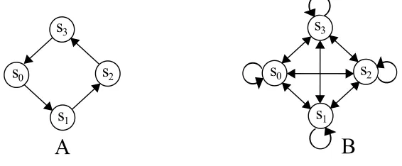
this empirically using the two tasks shown in Figure 8. Besides comparing against TD(λ), we also compare against experience replay (Lin, 1992), which stores the n last experience samples and uses them for repeated TD updates.

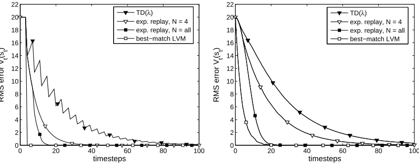
Task A features a small circular network consisting of four identical states, each having a de-terministic transition to a neighbor. The reward received after each transition is +1. Task B is a stochastic variation on the first task, with stochastic transitions and a reward drawn from a normal distribution with mean 1 and standard deviation 0.5. The discount factor is 0.95, resulting in a state value of 20 on both tasks for all states. We compare the RMS error of the current state value Vt(st)for all three methods. For experience replay, we performed a TD update for each of the last 4

samples at every timestep, resulting in a computation time similar to best-match LVM and TD(λ). In addition, we implemented a version where all observed samples are stored and updated at each timestep. The learning rate is initialized to 1 and decayed according to

αs₌ α0

d·[n(s)−1] +1.

where n(s)is the total number of times state s has been visited. We optimize d as well asλbetween 0 and 1. Results are averaged over 5000 runs.

Figure 8: Two tasks for policy evaluation. Task A has deterministic state transitions and a deter-ministic reward of +1, while task B has stochastic transitions and a reward drawn from a normal distribution with mean +1 and standard deviation 0.5.

(16)

0 20 40 60 80 100 0

2 4 6 8 10 12 14 16 18 20 22

timesteps

RMS error V

t

(s t

)

0 20 40 60 80 100

0 2 4 6 8 10 12 14 16 18 20 22

timesteps

RMS error V

t

(st

)

TD(λ)

exp. replay, N = 4 exp. replay, N = all best−match LVM

TD(λ)

exp. replay, N = 4 exp. replay, N = all best−match LVM

Figure 9: Comparison of the performance of best-match LVM, TD(λ) and experience replay on tasks A (left) and task B (right) of Figure 8.

to 80 ms for both best-match LVM and TD(λ). Experience replay with all samples updated had a computation time of 280 ms. On task B, all methods were about 10 ms slower.

4.3 Best-Match LVM Control

The best-match LVM equations for the control case form a nonlinear set. Therefore, it is in general not possible to compute the exact best-match Q-values at each timestep. However, they can be approximated to arbitrary accuracy via update sweeps through the state-action space, in a manner similar to value iteration, as we prove in the following lemma.

Lemma 9 For the best-match Q-values the following equation holds for all (s,a):

Q_tB(s,a) =lim

i→∞Qt,i(s,a),

where Qt,iis initialized arbitrarily for i=0 and is defined for i>0 as

Qt,i(s,a) = (

(1−α)Qtm f(s,a) +α[R′t(s,a) +γmaxa′Q_t_,_i₋_i(S′_t(s,a),a′)] if S′_t(s,a)6= /0

Qm ft (s,a) if S′t(s,a) = /0.

Proof For state-action pairs(s,a)with S′_t(s,a) =/0the proof follows directly from the definition of QB_t and Qt,i. For(s,a)with S′t(s,a)6=/0, the absolute difference between Qt,i(s,a)and QtB(s,a)can

be written as

|Qt,i(s,a)−QtB(s,a)| = αγ|max_c Qt,i−i(S′t(s,a),c)−max_c QtB(S′t(s,a),c)|

≤ αγmax

c |Qt,i−i(S

′

t(s,a),c)−QBt(S′t(s,a),c)|

(17)

From this it follows that

||Qt,i−QBt|| ≤αγ||Qt,i−i−QBt||.

Forαγ<1, it follows that for i→∞, Qt,i→QtB.

Lemma 9 shows that QB_t can be approximated to arbitrary accuracy with a finite number of best-match updates.

Algorithm 3 shows the pseudocode for a general class of algorithms that approximate the best-match Q-values by performing best-best-match updates.4 Lines 9 to 12 perform a series of best-match updates. Note that while only a single Qm f value is updated per timestep, many Q-values can be up-dated at the same timestep. By varying the way state-action pairs are selected for updating (line 10) and changing the stopping criterion (line 12), a whole range of algorithms can be constructed that trade off computation cost per timestep for better approximations of the best-match Q-values. Note that JIT Q-learning and even regular Q-learning are members of this general class of algorithms. If the state-action pair selection criterion is the state-action pair visited at the previous timestep and the stopping criterion allows only a single update, the algorithm reduces to the regular Q-learning algorithm. Thus, Q-learning is a form of best-match control with a simplistic approximation of the best-match Q-values. However, we reserve the term ‘best-match learning’ for algorithms that use the same sample multiple times to redo updates.

Algorithm 3 General Best-Match LVM Control

2: initialize S′(s,a) =/0for all s,a

4: initialize s

6: select action a, based on Q(s,·) 7: take action a, observe r and s′

8: Qm f(s,a)←Q(s,a); S′(s,a)←s′; R′(s,a)←r

9: repeat

10: select some(s¯,a¯)pair with S′(s¯,a¯)6= /0 {each pair is selected at least once before its revisit}

11: Q(s¯,a¯)←(1−αs ¯¯a₎_Qm f₍_s_¯_,_a_¯_{) +}αs ¯¯a_[_R′₍_s_¯_,_a_¯_{) +}_γ_max

cQ(S′(s¯,a¯),c)] 12: until some stopping criterion has been met

13: s←s′

15: end loop

The following theorem states that, for any member of the best-match LVM control class, the Q-values converge to the optimal Q-values.

Theorem 10 The Q-values of a member of the best-match LVM control class, shown in Algorithm 3, converge to Q∗if the following conditions are satisfied:

1. S and A are finite.

4. Similar to the variable Vrm f of Algorithm 2, a variable Qrm f can be defined that combines the variables Qm f and R′,

(18)

2. αt(s,a)∈[0,1],∑tαt(s,a) =∞,∑t(αt(s,a))2<∞w.p.1

andαt(s,a) =0 unless(s,a) = (st,at).

3. Var{R(s,a,s′)}<∞.

4. γ<1.

We prove this theorem in Appendix D.

4.4 Best-Match LVM Prioritized Sweeping

A wide range of methods can be constructed within the general class of best-match LVM control algorithms that trade off increased computation time for better approximation of the best-match Q-values in different ways. This section proposes one method that performs this trade-off with a strategy based on prioritized sweeping (PS) (Moore and Atkeson, 1993).

PS makes the planning step of model-based RL more efficient by focusing on the updates ex-pected to have the largest effect on the Q-value function. The algorithm maintains a priority queue of state-action pairs in consideration for updating. When a state-action pair(s,a)is updated, all predecessors (i.e., those state-action pairs whose estimated transition probabilities to s are greater than 0) are added to the queue according to a heuristic estimating the impact of the update. At each timestep, the top N state-action pairs from this queue are updated, with N depending on the available computation time. Because PS maintains a full model, it requires

O

(|

S

|2_|

_A

_|₎_space.

This same idea can be applied to the best-match equations for efficient approximation of the match values. A priority queue of state-action pairs is maintained whose corresponding best-match updates have the largest expected effect on the best-best-match Q-value estimates. When a state-action pair has received an update, all state-state-action pairs whose last-visit transition state equals the state from the updated state-action pair are placed into the priority queue with a priority equal to the absolute change an update would cause in its Q-value. Since this approach uses only an LVM, it requires only

O

(|

S

||

A

|)space.

Algorithm 4 shows the pseudocode of this algorithm, which we call best-match LVM prioritized sweeping (BM-LVM). By always putting the state-action pair from the previous timestep on top of the priority queue (line 10), the requirement that each visited state-action pair receives at least one best-match update is fulfilled, guaranteeing convergence in the limit.

On the surface, this algorithm resembles deterministic prioritized sweeping (DPS) (Sutton and Barto, 1998), a simpler variation that learns only a deterministic model, uses a slightly different priority heuristic, and performs Q-learning updates to its Q-values. While clearly designed for deterministic tasks, it can also be applied to stochastic tasks, in which case updates are based on an LVM.

However, there is a crucial difference between DPS and BM-LVM. By performing updates with respect to Qm f instead of Q, BM-LVM corrects previous updates instead of performing multiple updates based on the same sample. This ensures proper averaging of experience and enables con-vergence to the optimal Q-values using only an LVM, even in stochastic environments. This is not guaranteed for DPS since if some samples are used more often than others a bias towards these samples is created, which can prevent convergence to the optimal Q-values.

(19)

Algorithm 4 Best-Match LVM Prioritized Sweeping (BM-LVM)

2: initialize S′(s,a) =/0for all s,a

3: initialize PQueue as an empty queue

5: initialize s

7: select action a, based on Q(s,·) 8: Take action a, observe r and s′

9: S′(s,a)←s′; R′(s,a)←r; Qm f(s,a)←Q(s,a)

10: promote(s,a)to top of priority queue

11: n←0

12: while(n<N)∧(PQueue is not empty) do

13: s1,a1← f irst(PQueue)

14: Q(s1,a1)←(1−αs1a1)Qm f(s1,a1) +αs1a1[R′(s1,a1) +γmaxcQ(S′(s1,a1),c)]

15: Vs1 ←maxa′Q(s1,a

′₎

16: for all(s¯,a¯)with S′(s¯,a¯) =s1do

17: p← |(1−αs ¯¯a₎_Qm f₍_s_¯_,_a_¯_{) +}_αs ¯¯a_[_R′₍_s_¯_,_a_¯_{) +}_γ_V

s1]−Q(s¯,a¯)|

18: if p>θthen

19: insert(s¯,a¯)into PQueue with priority p

20: end if

21: end for

22: n←n+1

23: end while

24: s←s′

26: end loop

described by Watkins (1989). This is an off-policy control version of eligibility traces. We also tried Sarsa(λ), the on-policy version, since it can sometimes outperform Q(λ) considerably, but saw no significant difference for these experiments and present only the Q(λ) results. Note that when a greedy behavior policy is used, as in the deterministic experiment, Q(λ) computes exactly the same values as Sarsa(λ). As in Section 4.2, we also compare to experience replay.

Finally, we compare to delayed Q-learning (Strehl et al., 2006), a model-free method that, like some model-based methods (Brafman and Tennenholtz, 2002; Kearns and Singh, 2002; Strehl and Littman, 2005), is proven to be probably approximately correct (PAC), that is, its sample complex-ity is polynomial with high probabilcomplex-ity. Delayed Q-learning initializes its Q-values optimistically and ensures that value estimates are not reduced until the corresponding state-action pairs have been sufficiently explored. Because it does not maintain a model, it has the same

O

(|

S

||

A

|)space require-ments as best-match prioritized sweeping. However, to our knowledge, its empirical performance has never been evaluated before.

(20)

type (replacing versus accumulating). For delayed Q-learning we optimized m in the range from 1 to 5 with steps of 1 and e1in the range 0 to 0.020 with steps of 0.001. For DPS and BM-LVM, we did not optimize any parameters in the deterministic case, but simply used a constantαof 1. In the stochastic case, we also optimized the learning rate decay d for DPS and BM-LVM.

For all methods, we used optimistic initialization with Q0=20 in order to get a fair comparison with delayed Q-learning, for which initialization to Rmax/(1−γ)is part of the algorithm.5

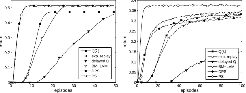
In the deterministic case we used a greedy behavior policy, while we used anε-greedy policy with ε=0.1 in the stochastic variant. For all prioritized-sweeping algorithms we performed a maximum of 20 updates per timestep (i.e., N = 20). For experience replay we used the last 20 samples, which also results in 20 updates per timestep. Results are averaged over 1000 independent runs.

0 10 20 30 40 50

0 0.1 0.2 0.3 0.4 0.5

episodes

return

0 20 40 60 80 100

0 0.05 0.1 0.15 0.2 0.25 0.3 0.35 0.4

episodes

return

Q(λ) exp. replay delayed Q BM−LVM DPS PS

Figure 10: Comparison of the performance of BM-LVM and several competitors on the determin-istic (left) and stochastic (right) Dyna Maze task.

Figure 10 shows the return as a function of the number of episodes, while Tables 2 and 3 show the average return over the measured episodes and the optimal parameter values. In the determinis-tic experiment, we see that the performance of PS, DPS, and BM-LVM is exactly equal, as expected whenα=1, since the last-visit experience is equal to the model of the environment. Q(λ) performs considerably worse than the prioritized sweeping methods and does not converge to the optimal pol-icy. In contrast, the combination of a greedy behavior policy with optimistic initialization enables the prioritized sweeping methods to converge to the optimal policy in a deterministic environment. Experience replay performs similarly to Q(λ), though it does converge to the optimal policy. De-layed Q-learning also converges to the optimal policy, as predicted by the theory, but does so much more slowly.

In the stochastic experiment, PS has a clear performance advantage. However, the goal of BM-LVM is not to match or even come close to the performance of PS. It cannot match this performance in general, since PS takes advantage of its higher space complexity. Instead, the goal of BM-LVM

5. For this task r=Rmaxonly when the exit is reached and 0 otherwise. Thus, the Q-values can never be higher than 1

and Q0=20 is overly optimistic. However, since realizing that an initialization of 1 is possible would require extra

(21)

deterministic - 50 eps.

optimal parameters average standard time per step return error (·10−6_s₎

Q(λ) λ: 0.8, d: 0 0.3606 0.0007 0.68

exp. replay d: 0 0.3602 0.0004 0.37

delayed Q m: 1, e1= 0 0.1878 0.0004 0.11

BM-LVM d: 0 0.4769 0.0002 0.88

DPS d: 0 0.4774 0.0002 0.85

PS - 0.4772 0.0002 0.95

Table 2: Average return and optimal parameters (d =αdecay rate) of best-match prioritized sweep-ing and several competitors on the deterministic Dyna Maze task.

stochastic - 100 eps.

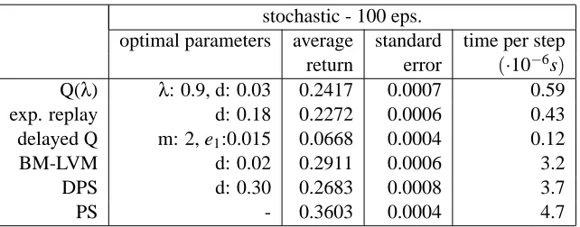
optimal parameters average standard time per step return error (·10−6_s₎ Q(λ) λ: 0.9, d: 0.03 0.2417 0.0007 0.59

exp. replay d: 0.18 0.2272 0.0006 0.43

delayed Q m: 2, e1:0.015 0.0668 0.0004 0.12

BM-LVM d: 0.02 0.2911 0.0006 3.2

DPS d: 0.30 0.2683 0.0008 3.7

PS - 0.3603 0.0004 4.7

Table 3: Average return and optimal parameters (d =αdecay rate) of best-match prioritized sweep-ing and several competitors on the stochastic Dyna Maze task.

is to optimally perform at a space complexity of

O

(|

S

||

A

|). The results confirm that BM-LVM is considerably better than the other methods with this space complexity, like Q(λ) and DPS. DPS initially performs well, but cannot keep up with LVM after about 10 episodes, even though BM-LVM has similar space and computation costs per timestep. Experience replay performs slightly worse than Q(λ). We tested whether doubling the size of the stored experience sequence improves the performance of experience replay, but this led to no significant performance increase. Delayed Q-learning also performs poorly in the stochastic case, despite its PAC bounds.

The computation time of BM-LVM, DPS and PS is in the deterministic experiment considerably lower than in the stochastic case. The reason for this is that while in both cases the maximum number of updates per timestep is 20, in the deterministic case the priority queue often has fewer than 20 samples, so fewer updates occur. The computation time of Q(λ) is slightly better than that of BM-LVM, while experience replay is about twice as fast as BM-LVM.

(22)

considerably better than the average return of Q(λ). This demonstrates that BM-LVM is a better choice than Q(λ) even under severe computational constraints.

Together, these results clearly demonstrate the strength of best-match learning, since BM-LVM outperforms several competitors with similar space complexity. However, the results also show that the performance gap with full model-based learning can be considerable. Therefore, if more space is available, a better approximate model would be preferred. We address this need in the next section by applying best-match learning to an n-transition model, which estimates the transition function for n next states per state-action pair, allowing increased space requirements to be traded for improved performance.

5. Best-Match n-Transition Model

The best-match LVM equations described above combine model-free Q-values with the last-visit model. When state-action pairs have only a small number of possible next states, the last-visit model can effectively approximate the full model. In other cases, however, the last-visit model captures only a fraction of the full model and the effect of the best-match updates will be small. In this section, we combine best-match learning with the n-transition model, which estimates the transition probability for n possible next states of each state-action pair. By tuning n, increased space requirements can be traded for improved performance.

5.1 Generalized Best-Match Equations

Best-match LVM learning takes the idea of using more accurate update targets to the extreme by continuously revising update targets with best-match updates. For a specific sample, the update target is revised until the moment of revisit of the corresponding state-action pair, since at that moment the sample is overwritten with the newly collected sample. However, if space allows, the new sample can be stored along with the old sample instead of overwriting it, allowing the update target from the new as well as the old sample to be further improved. We explain with an example how this changes the best-match equations.

6

Figure 11: A state transition sequence in which best-match updates can enable further postponing. Timesteps are shown below each state.

Consider the state-action sequence from Figure 11 and assume the best-match Q-values are computed at each timestep. At the revisit of sA, action a0is retaken. Therefore, when using the LVM, at timestep 5 the old experience sample is overwritten with the new experience. Before this occurs, the old experience is used in a final update of Qm f. Letυx_yindicate the update target from the sample collected at timestep x based on the best-match Q-value of timestep y: υx_y=rx+γmaxaQyB(sx,a).

Using this convention the update of Qm f at timestep 5 becomes

(23)

At timestep 7, the best-match LVM equation for(sA,a0)can be written as

Q₇B(sA,a0) = (1−α)Q7m f(sA,a0) +αυ57

= (1−α)Q₅m f(sA,a0) +αυ57

= (1−α)2Q₀m f(sA,a0) +α(1−α)υ14+αυ57.

Thus, the best-match Q-value of(sA,a0) at timestep 7 is equal to a weighted average of Q₀m f, υ14 andυ5₇. On the other hand, if both the old and the new sample are stored, Q-values from timestep 7 could also be used for the update target of the old sample, yielding

Q₇B(sA,a0) = (1−α)2Q₀m f(sA,a0) +α(1−α)υ17+αυ57. (10) For the state-sequence from Figure 11 this means that the experience resulting from(sB,a6)is also

taken into account in the update target for(sA,a0).

The above example shows how the best-match LVM equations can be naturally extended to two samples per state-action pair. Following the same pattern, we can define best-match equations given an arbitrary set of samples. Consider the set of samples X of size NX, where a sample x∈X has the

form{s,a,r,s′}. These samples can be grouped according to their state-action pairs. We define Xsa

as the subset of X containing all samples belonging to state-action pair(s,a)and N_sax as the size of Xsa. Without loss of generality, we index the samples from Xsaas xksafor 1≤k≤Nsax. In addition,

we define Wsaas a set consisting of Nsax +1 weights wksa∈IR such that 0≤wksa≤1 for 0≤k≤Nsax

and∑Nsax

k=0wksa=1. We define W as the union of the weight sets from all state-action pairs.

Definition 11 The generalized best-match equations with respect to Qtm f, X and W are

Q_tB(s,a) =w₀saQtm f(s,a) +w1saυ1sa+w2saυ2sa+...+wNsax

saυNsax , for all s,a , (11)

whereυ_ksa=r+γmaxcQBt(s′,c)|r,s′∈xksa.

Note that Equation 11 reduces to QB_t(s,a) =Qm ft (s,a)for state-action pairs with no samples in X .

Within this context, Qm f is defined as a model-free Q-value constructed from all observed sam-ples except those in X . Consequently, when a sample is removed from X , it is used for a model-free update of Qm f.

Using Definition 11, a range of algorithms can be constructed based on different sets of samples X and weights W . When the samples are combined by incremental Q-learning updates, like in Equation 10, the weights have the values

w₀sa = Nx

sa

∏

i=1

(1−α_isa), (12)

w_ksa = αsa k

Nx sa

∏

i=k+1

(1−αsa

i ), for 1≤k≤Nsax . (13)

(24)

all stored samples have the same time index so there is no reason to use different weights for them. A better weight distribution gives all samples the same weights:

w_ksa= (1−w₀sa)/N_sax , for 1≤k≤N_sax ,

for some value of w₀sa.

The last-visit model, storing one sample for each state-action pair, is one possible sample set. A straightforward extension is to store n samples per state-action pair. In the following section, however, we propose a different sample set, called the n-transition model, which can be stored more compactly.

5.2 Best-Match Learning based on the n-transition Model

While BM-LVM outperforms model-free methods with the same space complexity, it does not per-form as well as PS, which stores a full model. This is symptomatic of an important limitation of BM-LVM: it offers only a single trade-off between space and performance. When there is not enough space available to store the full model, but more than enough to store the LVM, a more sophisticated method is needed to make maximal use of the available space. Using the generalized best-match equations, we can construct such a method.

An obvious approach is to store n samples per state-action pair. However, obtaining an accurate model often requires a large n, even when the number of next states per state-action pair is small. A more space-efficient solution is to group together samples that have the same next state. If we store the size of such a group in N_sasx ′ and give each sample a weight of 1/Nsa, where Nsa is the

total number of times state-action pair(s,a)is visited, then we can rewrite the contribution from all samples of Xsato the best-match equations as

Nx sa

∑

k=1

wkυk=

1 Nsa

"

∑

X

rsa+γ

∑

s′

N_sasx ′max a′ Q

B₍_s′_,_a′₎

#

,

where∑Xrsais the sum of the rewards from all samples in the sample set belonging to(s,a). Using

w₀sa=1−N_sax/Nsa, ˆ

P

s ′

sa=Nsasx ′/N_sax and ˆ

R

_sa=∑_Xrsa/Nsax, the generalized best-match equations can

now be rewritten as

QB(s,a) =w₀saQm f(s,a) + (1−w₀sa) "

ˆ

R

_sa+γ

∑

s′

ˆ

P

_sas′max

a′ Q B₍_s′_,_a′₎

#

, for all s,a .

In these equations, ˆ

P

and ˆ

R

constitute a sparse, approximate model, whose size can be controlled by limiting the number of next states per state-action pair for which ˆ

P

is estimated. w₀sa is the fraction of all samples belonging to(s,a)not used by the sparse model. We define an n-transition model (NTM) to be one that estimates the transition probability ˆ

P

for n next states per state action pair. Once a sample enters the model, that is, is used to update ˆ

P

, it stays in the model. Each sample not used to update the model is used for a model-free update of Qm f. Different strategies can be used to determine which samples enter the model. A simple approach is to use the first n unique next states that are encountered for a specific state-action pair.