Blind Source Separation via Generalized Eigenvalue Decomposition
Lucas Parra [email protected]
Department of Biomedical Engineering The City College of New York
New York NY 10031, USA
Paul Sajda [email protected]
Department of Biomedical Engineering Columbia University
New York NY, 10027, USA
Editors: Te-Won Lee, Jean-Franc¸ois Cardoso, Erkki Oja and Shun-ichi Amari
Abstract
In this short note we highlight the fact that linear blind source separation can be formulated as a generalized eigenvalue decomposition under the assumptions of non-Gaussian, non-stationary, or non-white independent sources. The solution for the unmixing matrix is given by the generalized eigenvectors that simultaneously diagonalize the covariance matrix of the observations and an ad-ditional symmetric matrix whose form depends upon the particular assumptions. The method criti-cally determines the mixture coefficients and is therefore not robust to estimation errors. However it provides a rather general and unified solution that summarizes the conditions for successful blind source separation. To demonstrate the method, which can be implemented in two lines of matlab code, we present results for artificial mixtures of speech and real mixtures of electroencephalogra-phy (EEG) data, showing that the same sources are recovered under the various assumptions.
Keywords: blind source separation, generalized eigenvalue decomposition, Gaussian,
non-white, non-stationary
1. Introduction
The problem of recovering sources from their linear mixtures without knowledge of the mixing channel has been widely studied. In its simplest form it can be expressed as the problem of iden-tifying the factorization of the N-dimensional observations X into a mixing channel A and M-dimensional sources S,
X=AS. (1)
The T columns of the matrices X and S represent multiple samples. Often the samples in the data have a specific ordering such as consecutive samples in time domain signals or neighboring pixels in images. Without loss of generality we consider each column of X and S as a sample in time. In this case we can write Equation (1) as,
x(t) =As(t). (2)
that one can assume statistically independent sources. The resulting factorization is known as in-dependent component analysis (ICA) and was first introduced by Comon (1994). ICA makes no assumptions on the temporal structure of the sources. In this paper we consider additional assump-tions related to the statistical structure of neighboring samples. In these cases separation is also obtained for decorrelated sources.
We begin by noting that the matrix A explains various cross-statistics of the observations x(t)as an expansion of the corresponding diagonal cross-statistics of the sources s(t). An obvious example is the time averaged covariance matrix, Rx=∑tE[x(t)xH(t)],
Rx=ARsAH, (3)
where Rsis diagonal if we assume independent or decorrelated sources. In this paper we consider
the general case of complex-valued variables, and AHdenotes the Hermitian transpose of A. In the following section we highlight that for non-Gaussian, non-stationary, or non-white sources there exists, in addition to the covariance matrix, other cross-statistics Qswhich have the same
diagonal-ization property, namely,
Qx=AQsAH. (4)
Note that these two conditions alone are already sufficient for source separation. To recover the sources from the observation x(t) we must find an inverse matrix W such that WHA=I. In this case we have,
s(t) =WHAs(t) =WHx(t). (5)
Let us further assume nonzero diagonal values for Qs. After multiplying Equations (3) and (4) with
W and Equation (4) with Qs−1we combine them to obtain,
RxW=QxWΛ, (6)
where by assumption,Λ=RsQs−1, is a diagonal matrix. This constitutes a generalized eigenvalue
equation, where the eigenvalues represent the ratio of the individual source statistics measured by the diagonals of Rs and Qs. For distinct eigenvalues Equation (6) fully determines the unmixing
matrix WH specifying N column vectors corresponding to at most M =N sources. As with any
eigenvalue problem the order and scale of these eigenvectors is arbitrary. Hence, the recovered sources are arbitrary up to scale and permutations. This is also reflected in (5), where any scaling and permutation that is applied to the coordinates of s can be compensated by applying the inverse scales and permutations to the columns of W. A common choice to resolve these ambiguities is to scale the eigenvectors to unit norm, and to sort them by the magnitude of their generalized eigenvalues. For identical eigenvalues the corresponding sources are determined only up to rotations in the space spanned by the respective columns of W. If A is of rank M<N only the first M eigenvectors will
represent genuine sources while the remaining N−M eigenvectors span the subspace orthogonal to
A. This formulation therefore combines subspace analysis and separation into a single step. It does not, however, address the case of more sources than observations, i.e. M>N.
Incidentally, note that if we choose, Q=I, regardless of the observed statistic, Equation (4) reduces to the assumption of an orthonormal mixing, and the generalized eigenvalue equation re-duces to a conventional eigenvalue equation. The solutions are often referred to as the Principal Components of the observations x.
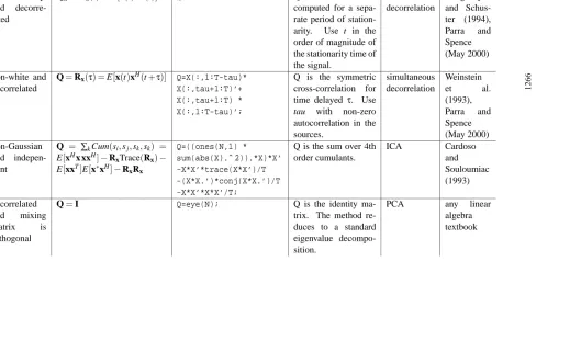
diagonal cross-statistics Q. A summary of the different assumptions and choices for Q is given in Table 1. We also show experimental results for signals that simultaneously satisfy the various assumptions. The results demonstrate that the method recovers the same set of underlying sources for different forms of Q.
2. Statistical Assumptions and the Form of Q
The independence assumption gives a set of conditions on the statistics of recovered sources. All cross-moments of independent variables factor, i.e.
E[sui(t)s∗jv(t+τ)] =E[siu(t)]E[s∗jv(t+τ)], i6= j, (7)
where E[.]represents the mathematical expectation, and∗is the complex conjugate. With (5) these equations define for each choice of{u,v,t,τ}a set of conditions on the coefficients of W and the observable statistics of x(t). With a sufficient number of such conditions the unknown parameters of W can be identified up to scale and permutation. Depending on the choice this implies that, in addition to independence, the sources are assumed to be either non-stationary, non-white, or
non-Gaussian as discussed in the next three sections.
2.1 Non-Stationary Sources
First, consider second order statistics, u+v=2, and sources with non-stationary power. The co-variance of the observations varies with the time t,
Rx(t) =E[x(t)xH(t)] =AE[s(t)sH(t)]AH=ARs(t)AH. (8)
Without restriction we assume throughout this paper zero mean signals.1 For zero mean signals Equation (7) implies that Rs(t) is diagonal. Therefore, A is a transformation that expands the
diagonal covariance of the sources into the observed covariance at all times. In particular, the sum over time leads to Equation (3) regardless of stationarity properties of the signals. Setting, Qx=Rx(t), for any time t, or linear combination of times, will give the diagonal cross-statistics
(4) required for the generalized eigenvalue Equation (6). Note that we have assumed non-stationary power. For sources that are spectrally non-stationary, but maintain a constant power profile, this approach is insufficient.
More generally, Equation (8) specifies for each t a set of N(N−1)/2 conditions on the NM unknowns in the matrix A. The unmixing matrix can be identified by simultaneously diagonalizing multiple covariance matrices estimated over different stationarity times. In the square case, N=M,
when using the generalized eigenvalue formulation, the N2parameters are critically determined by the N2 conditions in (6). To avoid the resulting sensitivity to estimation errors in the covariances Rx(t) it is beneficial to simultaneously diagonalize more than two matrices. This is discussed in
detail by Pham and Cardoso (2001).
2.2 Non-White Sources
For non-white sources (non-zero autocorrelation) one can use second order statistics in the form of cross-correlations for different time lagsτ:
Rx(τ) =E[x(t)xH(t+τ)] =AE[s(t)sH(t+τ)]AH=ARs(τ)AH. (9)
Here we assume that the signals are stationary such that the estimation is independent of t, or equivalently, that the expectation E[.] includes a time average. Again, (7) implies that Rs(τ) is
diagonal with the auto-correlation coefficients for lagτon its diagonal. Equation (9) has the same structure as (4) giving us for any choice ofτ, or linear combinations thereof, the required diagonal cross-statistics, Qx=Rx(τ), to obtain the generalized eigenvalue solution. The identification of
mixing channels using eigenvalue equations was first proposed by Molgedey and Schuster (1994) who suggested simultaneous diagonalization of cross-correlations. Time lagsτprovide new infor-mation if the source signals have distinct auto-correlations. Simultaneous diagonalization for more than two lags has been previously presented (Belouchrani et al., 1997).
2.3 Non-Gaussian Sources
For stationary and white sources different t andτdo not provide any new information. In that case (7) reduces to,
E[su
is∗jv] =E[sui]E[s∗jv], i6= j. (10)
To gain sufficient conditions one must include more than second order statistics of the data (u+m≥ 2). Consider for example 4th order cumulants expressed in terms of 4th order moments:
Cum(si,s∗j,sk,s∗l) =E[sis∗jsks∗l]−E[sis∗j]E[sks∗l]−E[sisk]E[s∗js∗l]−E[sis∗l]E[s∗jsk]. (11)
For Gaussian distributions all 4th order cumulants (11) vanish (Papoulis, 1991). In the follow-ing we assume non-zero diagonal terms and require therefore non-Gaussian sources. It is straight-forward to show using (10) that for independent variables the off-diagonal terms vanish, i6= j: Cum(si,s∗j,sk,s∗l) =0, for any k,l, i.e. the 4th order cumulants are diagonal in i,j for given k,l. Any
linear combination of these diagonal terms is also diagonal. Following the discussion by Cardoso and Souloumiac (1993) we define such a linear combination with coefficients, M={mlk},
ci j(M) =
∑
klCum(si,s∗j,sk,s∗l)mlk.
With Equation (11) and covariance, Rs=E[ssH], one can write in matrix notation:
Cs(M) =E[sHMs ssH]−RsTrace(MRs)−E[ssT]MTE[s∗sH]−RsMRs.
We have added the index s to differentiate from an equivalent definition for the observations x. Using the identity I this reads:
Cx(I) =E[xHx xxH]−RxTrace(Rx)−E[xxT]E[x∗xH]−RxRx. (12)
By inserting (2) into (12) it is easy to see that,
Since Cs(M) is diagonal for any M, it is also diagonal for M=AHA. We therefore find that A
expands the diagonal 4th order statistics to give the corresponding observable 4th order statistic Qx(I). This again gives us the required diagonal cross-statistics (4) for the generalized eigenvalue
decomposition. This method is instructive but very sensitive to estimation errors and the spread of kurtosis of the individual sources. For robust estimation simultaneous diagonalization using multiple Ms is recommended (Cardoso and Souloumiac, 1993).
3. Experimental Results
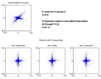
We first demonstrate, for an artificial mixture, that if a signal satisfies the various statistical assump-tions, the different choices for Q result in the same unmixing. Figure 1 shows an example where two speech signals were artificially mixed with a random mixing matrix A. 105 samples were used in this experiment. Speech satisfies all three statistical assumptions, namely it is stationary, non-white and non-Gaussian. The results show that the recovered source orientations are independent, and equivalent, for all three choices of Q.
−0.5 0 0.5
−0.5 0 0.5
mixed speech sources
−0.5 0 0.5
−0.5 0 0.5
non−stationary
−0.5 0 0.5
−0.5 0 0.5
non−white Results with Q assuming:
−0.5 0 0.5
−0.5 0 0.5
non−Gaussain % linear mix of sources S
X=A*S;
% Separation based on Generalized Eigenvalues [W,D]=eig(X*X’,Q);
S=W’ *X;
% linear mix of sources S X=A*S;
% Separation based on Generalized Eigenvalues [W,D]=eig(X*X’,Q);
S=W’ *X;
% linear mix of sources S X=A*S;
% Separation based on Generalized Eigenvalues [W,D]=eig(X*X’,Q);
S=W’ *X;
% linear mix of sources S X=A*S;
% Separation based on Generalized Eigenvalues [W,D]=eig(X*X’,Q);
S=W’ *X;
% linear mix of sources S X=A*S;
% Separation based on Generalized Eigenvalues [W,D]=eig(X*X’,Q);
S=W’ *X;
% linear mix of sources S X=A*S;
% Separation based on Generalized Eigenvalues [W,D]=eig(X*X’,Q);
S=W’ *X;
% linear mix of sources S X=A*S;
% Separation based on Generalized Eigenvalues [W,D]=eig(X*X’,Q);
S=W’ *X;
P A R R A A N D S A J D A Assuming sources are
Use MATLABcode Details Simple ver-sion of
References
non-stationary and decorre-lated
Qx=Rx(t) =E[x(t)xH(t)] Q=X(:,1:t)*X(:,1:t)’; Q is the covariance
computed for a sepa-rate period of station-arity. Use t in the order of magnitude of the stationarity time of the signal. simultaneous decorrelation Molgedey and Schus-ter (1994), Parra and Spence (May 2000) non-white and decorrelated
Q=Rx(τ) =E[x(t)xH(t+τ)] Q=X(:,1:T-tau)*
X(:,tau+1:T)’+ X(:,tau+1:T) * X(:,1:T-tau)’;
Q is the symmetric cross-correlation for time delayed τ. Use
tau with non-zero autocorrelation in the sources. simultaneous decorrelation Weinstein et al. (1993), Parra and Spence (May 2000) non-Gaussian and indepen-dent
Q = ∑kCum(si,sj,sk,sk) = E[xHx xxH]−R
xTrace(Rx)−
E[xxT]E[x∗xH]−R
xRx
Q=((ones(N,1) *
sum(abs(X).ˆ 2)).*X)*X’ -X*X’*trace(X*X’)/T -(X*X.’)*conj(X*X.’)/T -X*X’*X*X’/T;
Q is the sum over 4th order cumulants. ICA Cardoso and Souloumiac (1993) decorrelated and mixing matrix is orthogonal
Q=I Q=eye(N); Q is the identity
ma-trix. The method re-duces to a standard eigenvalue decompo-sition.
PCA any linear
algebra textbook
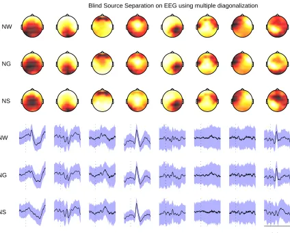
Results for real mixtures of EEG signals are shown in Figure 2. This data was collected as part of an error-related negativity (ERN) experiment (for details see Parra et al., 2002). To obtain robust estimates of the source directions we simultaneously diagonalized five or more cross-statistics, for a given condition, using the diagonalization algorithm by Cardoso and Souloumiac (1996).2 Sources with the largest generalized eigenvalues are shown in Figure 2. First note that for each of the three different statistical assumptions the same sources are recovered, as evidenced by the similarity in the scalp plots and their averaged time courses. It is clear that the same eight sources were selected among a posible 64 as having the largest generalized eigenvalue (with exeption of the last source in the non-stationary case). In addition, the spatial distribution of the first and fourth sources are readily identified as visual response (occipital) and and ERN (fronto-central) respectively. Fronto-central localization is indicative of the hypothesized origin of the ERN in the anterior cingulate (Dehaene et al., 1994). The consistent results, using different assumptions on the source statistics in combination with their functional neuroanatomical interpretation, is a validation of this approach. We note that others have attempted to recover EEG sources using a supervised method,3 which attempts to jointly diagonalize spatial sensor covariances for two different conditions, for example left and right motor imagery. This method, termed “common spatial patterns” (CSP) by Ramoser et al. (2000) can be seen as another example of the generalized eigenvalue decomposition, with the matrices Rxand Qxrepresenting the covariances for the two different conditions.
4. Conclusion
In this paper we formulate the problem of BSS as one of solving a generalized eigenvalue problem, where one of the matrices is the covariance matrix of the observations and the other is chosen based on the underlying statistical assumptions on the sources. This view unifies various approaches in simultaneous decorrelation and ICA, together with PCA and supervised methods such as CSP. Though in some cases the most straightforward implementation is not robust (e.g. see Table 1), we believe that it is a simple framework for understanding and comparing the various approaches, as well as a method for verifying the underlying statistical assumptions.
Acknowledgments
We would like to thank Clay Spence and Craig Fancourt for their help and discussions. This work was supported by the Defense Advanced Research Project Agency (DARPA) under contract N00014-01-C-0482. P.S. was also supported by the DoD Multidisciplinary University Research Initiative (MURI) program administered by the Office of Naval Research under grant N00014-01-1-0625 as well as an NSF CAREER Award (BES-0133804).
2. For an alternative diagonalization algorithm see also Yeredor (2002).
NW
NW
Blind Source Separation on EEG using multiple diagonalization
NG
NG NS
NS
0.8 s
References
A. Belouchrani, A.K. Meraim, J.-F. Cardoso, and E. Moulines. A blind source separation technique based on second order statistics. IEEE Trans. on Signal Processing, 45(2):434–444, February 1997.
J.-F. Cardoso and A. Souloumiac. Blind beamforming for non Gaussian signals. IEE Proceedings-F, 140(6):362–370, December 1993.
J.-F. Cardoso and A. Souloumiac. Jacobi angles for simultaneous diagonalization. SIAM J. Mat.
Anal. Appl., 17(1):161–164, January 1996.
P. Comon. Independent component analysis, a new concept? Signal Processing, 36(3):287–314, 1994.
S. Dehaene, M. Posner, and D. Tucker. Localization of a neural system for error detection ad compensation. Psychologic. Sci., 5:303–305, 1994.
L. Molgedey and H. G. Schuster. Separation of a mixture of independent signals using time delayed correlations. Phys. Rev. Lett., 72(23):3634–3637, 1994.
A. Papoulis. Probability, Random Variables, and Stochastic Processes. McGraw-Hill, 1991.
L. Parra, C. Alvino, A. Tang, B. Pearlmutter, N. Yeung, A. Osman, and P. Sajda. Linear spatial integration for single-trial detection in encephalography. Neuroimage, 17:223–230, 2002.
L. Parra and C. Spence. Convolutive blind source separation of non-stationary sources. IEEE Trans.
on Speech and Audio Processing, pages 320–327, May 2000.
D.-T. Pham and J.-F. Cardoso. Blind separation of instantaneous mixtures of non stationary sources.
IEEE Trans. Signal Processing, 49(9):1937–1848, 2001.
H. Ramoser, J. Mueller-Gerking, and G. Pfurtscheller. Optimal spatial filtering of single trial EEG during imagined hand movements. IEEE Trans. Rehab. Engng., 8(4):441–446, 2000.
E. Weinstein, M. Feder, and A.V. Oppenheim. Multi-channel signal separation by decorrelation.
IEEE Trans. Speech Audio Processing, 1(4):405–413, Apr. 1993.