Pairwise Support Vector Machines and their Application to Large Scale Problems

Pairwise Support Vector Machines and their Application to Large

Scale Problems

Carl Brunner [email protected]

Andreas Fischer [email protected]

Institute for Numerical Mathematics Technische Universit¨at Dresden 01062 Dresden, Germany

Klaus Luig [email protected]

Thorsten Thies [email protected]

Cognitec Systems GmbH Grossenhainer Str. 101 01127 Dresden, Germany

Editor:Corinna Cortes

Abstract

Pairwise classification is the task to predict whether the examplesa,bof a pair(a,b)belong to the same class or to different classes. In particular, interclass generalization problems can be treated in this way. In pairwise classification, the order of the two input examples should not affect the classification result. To achieve this, particular kernels as well as the use of symmetric training sets in the framework of support vector machines were suggested. The paper discusses both approaches in a general way and establishes a strong connection between them. In addition, an efficient im-plementation is discussed which allows the training of several millions of pairs. The value of these contributions is confirmed by excellent results on the labeled faces in the wild benchmark.

Keywords: pairwise support vector machines, interclass generalization, pairwise kernels, large scale problems

1. Introduction

To extend binary classifiers to multiclass classification several modifications have been suggested, for example the one against all technique, the one against one technique, or directed acyclic graphs, see Duan and Keerthi (2005), Hill and Doucet (2007), Hsu and Lin (2002), and Rifkin and Klautau (2004) for further information, discussions, and comparisons. A more recent approach used in the field of multiclass and binary classification is pairwise classification (Abernethy et al., 2009; Bar-Hillel et al., 2004a,b; Bar-Bar-Hillel and Weinshall, 2007; Ben-Hur and Noble, 2005; Phillips, 1999; Vert et al., 2007). Pairwise classification relies on two input examples instead of one and predicts whether the two input examples belong to the same class or to different classes. This is of particular advantage if only a subset of classes is known for training. For later use, a support vector machine (SVM) that is able to handle pairwise classification tasks is called pairwise SVM.

et al. (2004a) propose the use of training sets with a symmetric structure. We will discuss both approaches to obtain symmetry in a general way. Based on this, we will provide conditions when these approaches lead to the same classifier. Moreover, we show empirically that the approach of using selected kernels is three to four times faster in training.

A typical pairwise classification task arises in face recognition. There, one is often interested in the interclass generalization, where none of the persons in the training set is part of the test set. We will demonstrate that training sets with many classes (persons) are needed to obtain a good performance in the interclass generalization. The training on such sets is computationally expensive. Therefore, we discuss an efficient implementation of pairwise SVMs. This enables the training of pairwise SVMs with several millions of pairs. In this way, for the labeled faces in the wild database, a performance is achieved which is superior to the current state of the art.

This paper is structured as follows. In Section 2 we give a short introduction to pairwise clas-sification and discuss the symmetry of decision functions obtained by pairwise SVMs. Afterwards, in Section 3.1, we analyze the symmetry of decision functions from pairwise SVMs that rely on symmetric training sets. The new connection between the two approaches for obtaining symme-try is established in Section 3.2. The efficient implementation of pairwise SVMs is discussed in Section 4. Finally, we provide performance measurements in Section 5.

The main contribution of the paper is that we show the equivalence of two approaches for obtain-ing a symmetric classifier from pairwise SVMs and demonstrate the efficiency and good interclass generalization performance of pairwise SVMs on large scale problems.

2. Pairwise Classification

Let X be an arbitrary set and letm training examples xi ∈X with i∈M≔{1, . . . ,m} be given.

The class of a training example might be unknown, but we demand that we know for each pair (xi,xj) of training examples whether its examples belong to the same class or to different classes.

Accordingly, we defineyi j ≔+1 if the examples of the pair(xi,xj) belong to the same class and

call it apositive pair. Otherwise, we setyi j≔−1 and call(xi,xj)anegative pair.

In pairwise classification the aim is to decide whether the examples of a pair (a,b)∈X×X

belong to the same class or not. In this paper, we will make use of pairwise decision functions

f :X×X →R. Such a function predicts whether the examples a,bof a pair(a,b) belong to the same class (f(a,b)>0) or not (f(a,b)<0). Note that neither a,b need to belong to the set of training examples nor the classes ofa,bneed to belong to the classes of the training examples.

A common tool in machine learning are kernelsk:X×X→R. Let

H

H

k(s,t)≔hφ(s),φ(t)i

defines astandardkernel.

In pairwise classification one often uses pairwisekernelsK:(X×X)×(X×X)→R. In this paper we assume that any pairwise kernel is symmetric, that is, it holds that

K((a,b),(c,d)) =K((c,d),(a,b))

for alla,b,c,d∈X, and that it is positive semidefinite (Sch¨olkopf and Smola, 2001). For instance,

KD((a,b),(c,d))≔k(a,c) +k(b,d), (1)

are symmetric and positive semidefinite. We call KD direct sum pairwise kernel and KT tensor

pairwise kernel(cf. Sch¨olkopf and Smola, 2001).

A natural and desirable property of any pairwise decision function is that it should be symmetric in the following sense

f(a,b) = f(b,a) for alla,b∈X.

Now, let us assume thatI⊆M×Mis given. Then, the pairwise decision function f obtained by a pairwise SVM can be written as

f(a,b)≔

∑

αi jyi jK((xi,xj),(a,b)) +γ (3)

with bias γ∈Randαi j ≥0 for all (i,j)∈I. Obviously, if KD (1) or KT (2) are used, then the decision function is not symmetric in general. This motivates us to call a kernelK balancedif

K((a,b),(c,d)) =K((a,b),(d,c)) for alla,b,c,d∈X

holds. Thus, if a balanced kernel is used, then (3) is always a symmetric decision function. For instance, the following kernels are balanced

KDL((a,b),(c,d))≔ 1

2(k(a,c) +k(a,d) +k(b,c) +k(b,d)), (4)

KT L((a,b),(c,d))≔ 1

2(k(a,c)k(b,d) +k(a,d)k(b,c)), (5)

KML((a,b),(c,d))≔

1

4(k(a,c)−k(a,d)−k(b,c) +k(b,d))

2

, (6)

KT M((a,b),(c,d))≔KT L((a,b),(c,d)) +KML((a,b),(c,d)). (7)

Vert et al. (2007) callKMLmetric learning pairwise kernel andKT Ltensor learning pairwise

ker-nel. Similarly, we callKDL, which was introduced in Bar-Hillel et al. (2004a),direct sum learning

pairwise kernelandKT M tensor metric learning pairwise kernel. For representing some balanced

kernels by projections see Brunner et al. (2011).

3. Symmetric Pairwise Decision Functions and Pairwise SVMs

Pairwise SVMs lead to decision functions of the form (3). As detailed above, if a balanced kernel is used within a pairwise SVM, one always obtains a symmetric decision function. For pairwise SVMs which useKD(1) as pairwise kernel, it has been claimed that any symmetric set of training

pairs leads to a symmetric decision function (see Bar-Hillel et al., 2004a). We call a set of training pairs symmetric, if for any training pair (a,b) the pair (b,a) also belongs to the training set. In Section 3.1 we prove the claim of Bar-Hillel et al. (2004a) in a more general context which includes

KT (2). Additionally, we show in Section 3.2 that under some conditions a symmetric training

3.1 Symmetric Training Sets

In this subsection we show that the symmetry of a pairwise decision function is indeed achieved by means of symmetric training sets. To this end, letI⊆M×Mbe a symmetric index set, in other words if(i,j)belongs toIthen(j,i)also belongs toI. Furthermore, we will make use of pairwise kernelsKwith

K((a,b),(c,d)) =K((b,a),(d,c)) for alla,b,c,d∈X. (8)

As any pairwise kernel is assumed to be symmetric, (8) holds for any balanced pairwise kernel. Note that there are other pairwise kernels that satisfy (8), for instance for the kernels given in Equations 1 and 2.

ForIR,IN⊆I defined byIR≔{(i,j)∈I|i= j}andIN≔I\IRlet us consider the dual pairwise

SVM

min α G(α)

s. t. 0≤αi j≤C for all(i,j)∈IN

0≤αii≤2C for all(i,i)∈IR

∑

(i,j)∈I

yi jαi j=0.

(9)

with

G(α)≔1

2_(i,j)

∑

∑

Lemma 1 If I is a symmetric index set and if (8) holds, then there is a solution αˆ of (9) with

ˆ

αi j=αˆjifor all(i,j)∈I.

Proof By the theorem of Weierstrass there is a solutionα∗ of (9). Let us define another feasible point ˜αof (9) by

˜

αi j≔α∗ji for all(i,j)∈I.

For easier notation we setKi j,kl≔K((xi,xj),(xk,xl)). Then,

2G(α˜) =

_∑

(i,j),(k,l)∈I

α∗_jiα∗_lkyi jyklKi j,kl−2

∑

α∗_ji.

Note thatyi j=yjiholds for all(i,j)∈I. By (8) we further obtain

2G(α˜) =

_∑

(i,j),(k,l)∈I

α∗_jiα∗_lkyjiylkKji,lk−2

∑

α∗_ji= 2G(α∗).

The last equality holds sinceIis a symmetric training set. Hence, ˜αis also a solution of (9). Since (9) is convex (cf. Sch¨olkopf and Smola, 2001),

αλ≔λα∗+ (1−λ)α˜

solves (9) for anyλ∈[0,1]. Thus, ˆα≔α1/2has the desired property.

Theorem 2 If I is a symmetric index set and if (8)holds, then any solutionα of the optimization problem(9)leads to a symmetric pairwise decision function f :X×X→R.

Proof For any solutionαof (9) let us definegα:X×X →Rby

gα(a,b)≔

∑

αi jyi jK((xi,xj),(a,b)).

Then, the obtained decision function can be written as fα(a,b) =gα(a,b) +γfor some appropriate

γ∈R. Ifα

1 _andα2 _{are solutions of (9) theng}

α1 =g_α2 can be derived by means of convex

opti-mization theory. According to Lemma 1 there is always a solution ˆα of (9) with ˆαi j =αˆjifor all

(i,j)∈I. Obviously, such a solution leads to a symmetric decision function fαˆ. Hence, fα is a symmetric decision function for all solutionsα.

3.2 Balanced Kernels vs. Symmetric Training Sets

Section 2 shows that one can use balanced kernels to obtain a symmetric pairwise decision function by means of a pairwise SVM. As detailed in Section 3.1 this can also be achieved by symmet-ric training sets. Now, we show in Theorem 3 that the decision function is the same, regardless whether a symmetric training set or a certain balanced kernel is used. This result is also of practical value, since the approach with balanced kernels leads to significantly shorter training times (see the empirical results in Section 4.2).

SupposeJis a largest subset of a given symmetric index setI satisfying

((i,j)∈J∧j6=i) ⇒ (j,i)∈/J.

Now, we consider the optimization problem

min β H(β)

s. t. 0≤βi j ≤2C for all(i,j)∈J

∑

(i,j)∈J

yi jβi j=0

(10)

with

H(β)≔1

2_(i,j),

∑

∑

and

ˆ

Ki j,kl≔

1

2 Ki j,kl+Kji,kl

, (11)

whereKis an arbitrary pairwise kernel. Obviously, ˆKis a balanced kernel. For instance, ifK=KD

(1) then ˆK=KDL(4) or ifK=KT (2) then ˆK=KT L(5). The assumed symmetry ofKyields

ˆ

Ki j,kl=Kˆi j,lk=Kˆji,kl=Kˆji,lk=Kˆkl,i j=Kˆlk,i j=Kˆkl,ji=Kˆlk,ji. (12)

Theorem 3 Let the functions gα:X×X→Rand hβ:X×X→Rbe defined by

gα(a,b)≔

∑

αi jyi jK((xi,xj),(a,b)),

hβ(a,b)≔

∑

βi jyi jKˆ((xi,xj),(a,b)),

where I is a symmetric index set and J is defined as above. Additionally, let K fulfill(8)andK beˆ given by(11). Then, for any solutionα∗of (9)and for any solutionβ∗of(10)it holds that gα∗=h_β∗.

Proof By means of convex optimization theory it can be derived thatgαis the same function for any solutionα. The same holds forhβand any solutionβ. Hence, due to Lemma 1 we can assume thatα∗is a solution of (9) withα∗_{i j} =α∗_ji. ForJR≔IR andJN≔J\JR we define ¯βby

¯

βi j≔

α∗_{i j}+α∗_ji if(i,j)∈JN,

α∗_ii if(i,j)∈JR.

Obviously, ¯βis a feasible point of (10). Then, by (11) and byα∗

i j =α∗jiwe obtain for

(i,j)∈JN: β¯i jKˆi j,kl=

¯

βi j

2 (Ki j,kl+Kji,kl) =

α∗ i j+α∗ji

2 Ki j,kl+Kji,kl

=α∗_{i j}Ki j,kl+α∗jiKji,kl,

(i,i)∈JR: β¯iiKˆii,kl=

¯

βii

2 (Kii,kl+Kii,kl) =α

∗ iiKii,kl.

(13)

Then,yi j=yjiimplies

h_β¯=gα∗. (14)

In a second step we prove that ¯βis a solution of problem (10). By usingykl=ylk, the symmetry

ofK, (13), (12), and the definition of ¯βone obtains

2G(α∗) +2

∑

(i,j)∈I

α∗_{i j}

=

_∑

(i,j)∈I

α∗_{i j}yi j

∑

ykl α∗klKi j,kl+α∗lkKi j,lk

+

_∑

(k,k)∈JR

ykkα∗kkKi j,kk

!

=

_∑

(i,j)∈JN∪JR

α∗_{i j}yi j

∑

¯

βklyklKˆi j,kl+

∑

α∗_jiyji

∑

¯

βklyklKˆji,kl

=

_∑

(i,j)∈JN

¯

βi jyi j

∑

¯

βklyklKˆi j,kl+

∑

¯

βiiyii

∑

¯

βklyklKˆii,kl

=2H(β¯) +2

∑

(i,j)∈J

¯

βi j.

Then, the definition of ¯βimplies

Now, let us define ¯αby

¯

αi j≔







β∗_{i j}/2 if(i,j)∈JN,

β∗_ji/2 if(j,i)∈JN,

β∗_ii if(i,j)∈JR.

Obviously, ¯αis a feasible point of (9). Then, by (8) and (11) we obtain for

(k,l)∈JN: α¯klKi j,kl+α¯lkKi j,lk=

β∗_kl

2 (Ki j,kl+Ki j,lk) =β

∗ klKˆi j,kl,

(k,k)∈JR: α¯kkKi j,kk=

β∗ kk

2 (Ki j,kk+Ki j,kk) =β

∗ kkKˆi j,kk.

This, (12), andykl=ylkyield

2H(β∗) +2

∑

(i,j)∈J

β∗_{i j}

=

_∑

(i,j)∈J

β∗_{i j}yi j

∑

β∗_klykl

1

2 Kˆi j,kl+Kˆji,kl

+

_∑

(k,k)∈JR

β∗_kkykk

1

2 Kˆi j,kk+Kˆji,kk

!

=1

2_(i,

∑

∗

i jyi j

∑

¯

αklykl Ki j,kl+Kji,kl

!

.

Then, the definition of ¯αprovidesβ∗

i j=α¯i j+α¯jifor(i,j)∈JNand ¯αi j=α¯ji. Thus,

2H(β∗) +2

∑

(i,j)∈J

β∗_{i j}=

_∑

(i,j)∈I

¯

αi jyi j

∑

¯

αklyklKi j,kl

!

=2G(α¯) +2

∑

(i,j)∈I

¯

αi j

follows. This impliesG(α¯) =H(β∗_{). Now, let us assume that ¯βis not a solution of (10). Then,} H(β∗_)<H(β¯_{)holds and, by (15), we have}

G(α∗) =H(β¯)>H(β∗) =G(α¯).

This is a contradiction to the optimality ofα∗_{. Hence, ¯βis a solution of (10) andh}

β∗ =h_β¯ follows.

Then, with (14) we have the desired result.

4. Implementation

4.1 Caching the Standard Kernel

In this subsection balanced kernels are used to enforce the symmetry of the pairwise decision func-tion. Kernel evaluations are crucial for the performance of LIBSVM. If we could cache the whole kernel matrix in RAM we would get a huge increase of speed. Today, this seems impossible for sig-nificantly more than 125,250 training pairs as storing the (symmetric) kernel matrix for this number of pairs in double precision needs approximately 59GB. Note that training sets with 500 training examples already result in 125,250 training pairs. Now, we describe how the costs of kernel eval-uations can be drastically reduced. For example, let us select the kernelKT L(5) with an arbitrary

standard kernel. For a single evaluation ofKT Lthe standard kernel has to be evaluated four times

with vectors ofX. Afterwards, four arithmetic operations are needed.

It is easy to see that each standard kernel value is used for evaluating many different elements of the kernel matrix. In general, it is possible to cache the standard kernel values for all training examples. For example, to cache the standard kernel values for 10,000 examples one needs 400MB. Thus, each kernel evaluation ofKT Lcosts four arithmetic operations only. This does not depend on

the chosen standard kernel.

Table 1 compares the training times with and without caching the standard kernel values. For these measurements examples from the double interval task (cf. Section 5.1) are used where each class is represented by 5 examples,KT Lis chosen as pairwise kernel with a linear standard kernel, a

cache size of 100MB is selected for caching pairwise kernel values, and all possible pairs are used for training. In Table 1a the training set of each run consists ofm=250 examples of 50 classes with different dimensionsn. Table 1b shows results for different numbersmof examples of dimension

n=500. The speedup factor by the described caching technique is up to 100.

Dimension Standard kernel

nof (time in mm:ss)

examples not cached cached

200 2:08 0:07

400 4:31 0:07

600 6:24 0:07

800 9:41 0:08

1000 11:27 0:09

(a) Different dimensionsnof examples

Number Standard kernel

mof (time in hh:mm)

examples not cached cached

200 0:04 0:00

400 1:05 0:01

600 4:17 0:02

800 12:40 0:06

1000 28:43 0:13

(b) Different numbersmof examples

Table 1: Training time with and without caching the standard kernel

4.2 Balanced Kernels vs. Symmetric Training Sets

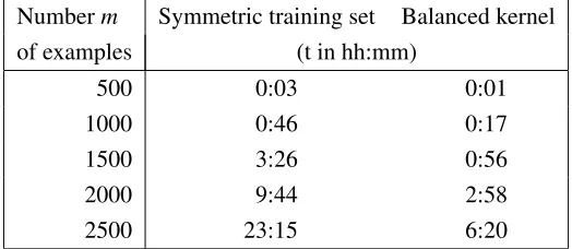
Table 2 compares the needed training time of both approaches. There, examples from the double interval task (cf. Section 5.1) of dimensionn=500 are used where each class is represented by 5 examples, KT and its balanced version KT L with linear standard kernels are chosen as pairwise

kernel, a cache size of 100MB is selected for caching the pairwise kernel values, and all possible pairs are used for training. It turns out, that the approach with balanced kernels is three to four times faster than using symmetric training sets. Of course, the technique of caching the standard kernel values as described in Section 4.1 is used within all measurements.

Numberm Symmetric training set Balanced kernel

of examples (t in hh:mm)

500 0:03 0:01

1000 0:46 0:17

1500 3:26 0:56

2000 9:44 2:58

2500 23:15 6:20

Table 2: Training time for symmetric training sets and for balanced kernels

5. Classification Experiments

In this section we will present results of applying pairwise SVMs to one synthetic data set and to one real world data set. Before we come to those data sets in Sections 5.1 and 5.2 we introduceK_{T L}lin

andK_{T L}poly. Those kernels denoteKT L (5) with linear standard kernel and homogenous polynomial

standard kernel of degree two, respectively. The kernels K_MLlin, K_MLpoly, K_{T M}lin, and K_{T M}poly are defined analogously. In the following, detection error trade-off curves (DET curves cf. Gamassi et al., 2004) will be used to measure the performance of a pairwise classifier. Such a curve shows for any false match rate (FMR) the corresponding false non match rate (FNMR). A special point of interest of such a curve is the (approximated) equal error rate (EER), that is the value for which FMR=FNMR holds.

5.1 Double Interval Task

Let us describe thedouble interval taskof dimensionn. To get such an examplex∈ {−1,1}n_one

drawsi,j,k,l∈Nso that 2≤i≤ j,j+2≤k≤l≤nand defines

xp≔

1 p∈ {i, . . . ,j} ∪ {k, . . . ,l},

−1 otherwise.

The classcof such an example is given byc(x)≔(i,k). Note that the pair(j,l)does not influence

the class. Hence, there are(n−3)(n−2)/2 classes.

0 0.1 0.2 0.3 0.4 0.5 0.6 0.7 0.8 0.9 1

0.001 0.01 0.1 1

F N M R FMR Klin

M L50 Classes

Klin

M L100 Classes

Klin

M L200 Classes

KpolyT M50 Classes

KT Mpoly100 Classes

KT Mpoly200 Classes

(a) Different class numbers in training

0 0.1 0.2 0.3 0.4 0.5 0.6 0.7 0.8 0.9 1

0.001 0.01 0.1 1

F N M R FMR Klin M L Kpoly M L Klin T L

KT Lpoly

Klin T M

KT Mpoly

(b) Different kernels for 200 classes in training

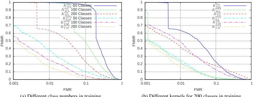
Figure 1: DET curves for double interval task

set of classes in the test set. We created training sets consisting of 50 classes and different numbers of examples per class. For training all possible training pairs were used.

We observed that an increasing number of examples per class improves the performance inde-pendently of the other parameters. As a trade-off between the needed training time and performance of the classifier, we decided to use 15 examples per class for the measurements. Independently of the selected kernel, a penalty parameterCof 1,000 turned out to be a good choice. The kernelKDS

led to a bad performance regardless of the standard kernel chosen. Therefore, we omit results for

KDS.

Figure 1a shows that an increasing number of classes in the training set improves the perfor-mance significantly. This holds for all kernels mentioned above. Here, we only present results for

K_MLlin andK_{T M}poly. Figure 1b shows the DET curves for different kernels where the training set consists of 200 classes. In particular, any of the pairwise kernels which uses a homogeneous polynomial of degree 2 as standard kernel leads to better results than its corresponding counterpart with a linear standard kernel. For FMRs smaller than 0.07 K_{T M}poly leads to the best results, whereas for larger FMRs the DET curves ofK_MLpoly,K_{T L}poly, andK_{T M}polyintersect.

5.2 Labeled Faces in the Wild

In this subsection we will present results of applying pairwise SVMs to the labeled faces in the wild (LFW) data set (Huang et al., 2007). This data set consists of 13,233 images of 5,749 persons. Several remarks on this data set are in order. Huang et al. (2007) suggest two protocols for perfor-mance measurements. Here, the unrestricted protocol is used. This protocol is a fixed tenfold cross validation where each test set consists of 300 positive pairs and 300 negative pairs. Moreover, any person (class) in a training set is not part of the corresponding test set.

0 0.1 0.2 0.3 0.4 0.5 0.6 0.7 0.8 0.9 1

0.001 0.01 0.1 1

F N M R FMR Klin M L Kpoly M L Klin T L

KT Lpoly

Klin T M

KT Mpoly

(a) View 1 partition, different kernels, added up decision function values of SIFT, LPB, and TPLBP feature vectors

0 0.1 0.2 0.3 0.4 0.5 0.6 0.7 0.8 0.9

0.001 0.01 0.1 1

F N M R FMR SIFT LBP TPLBP LBP+TPLBP SIFT+LBP+TPLBP

(b) Unrestricted protocol,K_{T M}poly, different feature vectors, “+” stands for adding up the corresponding decision func-tion values

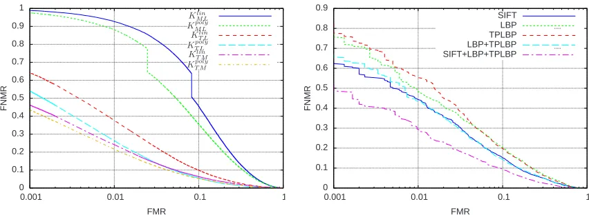
Figure 2: DET curves for LFW data set

local binary patterns (LBP) (Ojala et al., 2002) and three-patch LBP (TPLBP) (Wolf et al., 2008) are extracted. In contrast to Li et al. (2012), the pose is neither estimated nor swapped and no PCA is applied to the data. As the norm of the LBP feature vectors is not the same for all images we scaled them to Euclidean norm 1.

For model selection, the View 1 partition of the LFW database is recommended (Huang et al., 2007). Using all possible pairs of this partition for training and for testing, we obtained that a penalty parameterCof 1,000 is suitable. Moreover, for each used feature vector, the kernelK_{T M}poly leads to the best results among all used kernels and also if sums of decision function values belonging to SIFT, LBP, and TPLBP feature vectors are used. For example, Figure 2a shows the performance of different kernels, where the decision function values corresponding to SIFT, LBP, and TPLBP feature vectors are added up.

Due to the speed up techniques presented in Section 4 we were able to train with large numbers of training pairs. However, if all pairs were used for training, then any training set would consist of approximately 50,000,000 pairs and the training would still need too much time. Hence, whereas in any training set all positive training pairs were used, the negative training pairs were randomly selected in such a way that any training set consists of 2,000,000 pairs. The training of such a model took less than 24 hours on a standard PC. In Figure 2b we present the average DET curves obtained for K_{T M}poly and feature vectors based on SIFT, LBP, and TPLBP. Inspired by Li et al. (2012), we determined two further DET curves by adding up the decision function values. This led to very good results. Furthermore, we concatenated the SIFT, LBP, and TPLBP feature vectors. Surprisingly, the training of some of those models needed longer than a week. Therefore, we do not present these results.

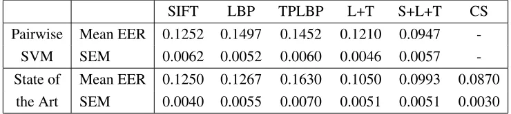
pairwise SVMs we achieved the same EER but a slightly higher SEM 0.1252±0.0062. If we add up the decision function values corresponding to the LBP and TPLBP feature vectors, then our result 0.1210±0.0046 is worse compared to the state of the art 0.1050±0.0051. One possible reason for this fact might be that we did not swap the pose. Finally, for the added up decision function values corresponding to SIFT, LBP and TPLBP feature vectors, our performance 0.0947±0.0057 is better than 0.0993±0.0051. Furthermore, it is worth noting that our standard errors of the mean are comparable to the other presented learning algorithms although most of them use a PCA to reduce noise and dimension of the feature vectors. Note that the results of the commercial system are not directly comparable since it uses outside training data (for reference see Huang et al., 2007).

SIFT LBP TPLBP L+T S+L+T CS

Pairwise Mean EER 0.1252 0.1497 0.1452 0.1210 0.0947

-SVM SEM 0.0062 0.0052 0.0060 0.0046 0.0057

-State of Mean EER 0.1250 0.1267 0.1630 0.1050 0.0993 0.0870

the Art SEM 0.0040 0.0055 0.0070 0.0051 0.0051 0.0030

Table 3: Mean EER and SEM for LFW data set. S=SIFT, L=LBP, T=TPLBP, +=adding up decision

function values, CS=Commercial systemface.com r2011b

6. Final Remarks

In this paper we suggested the SVM framework for handling large pairwise classification problems. We analyzed two approaches to enforce the symmetry of the obtained classifiers. To the best of our knowledge, we gave the first proof that symmetry is indeed achieved. Then, we proved that for each parameter set of one approach there is a corresponding parameter set of the other one such that both approaches lead to the same classifier. Additionally, we showed that the approach based on balanced kernels leads to shorter training times.

We discussed details of the implementation of a pairwise SVM solver and presented numerical results. Those results demonstrate that pairwise SVMs are capable of successfully treating large scale pairwise classification problems. Furthermore, we showed that pairwise SVMs compete very well for a real world data set.

We would like to underline that some of the discussed techniques could be transferred to other approaches for solving pairwise classification problems. For example, most of the results can be applied easily to One Class Support Vector Machines (Sch¨olkopf et al., 2001).

Acknowledgments

References

J. Abernethy, F. Bach, T. Evgeniou, and J.-P. Vert. A new approach to collaborative filtering: Oper-ator estimation with spectral regularization.Journal of Machine Learning Research, 10:803–826, 2009.

A. Bar-Hillel and D. Weinshall. Learning distance function by coding similarity. In Z. Ghahramani, editor,Proceedings of the 24th International Conference on Machine Learning (ICML ’07), pages 65–72. ACM, 2007.

A. Bar-Hillel, T. Hertz, and D. Weinshall. Boosting margin based distance functions for cluster-ing. In C. E. Brodley, editor, In Proceedings of the 21st International Conference on Machine Learning (ICML ’04), pages 393–400. ACM, 2004a.

A. Bar-Hillel, T. Hertz, and D. Weinshall. Learning distance functions for image retrieval. In Pro-ceedings of the IEEE Computer Society Conference on Computer Vision and Pattern Recognition (CVPR ’04), volume 2, pages 570–577. IEEE Computer Society Press, 2004b.

A. Ben-Hur and W. Stafford Noble. Kernel methods for predicting protein–protein interactions.

Bioinformatics, 21(1):38–46, 2005.

C. Brunner, A. Fischer, K. Luig, and T. Thies. Pairwise kernels, support vector machines, and the application to large scale problems. Technical Report MATH-NM-04-2011, In-stitute of Numerical Mathematics, Technische Universit¨at Dresden, October 2011. URL

http://www.math.tu-dresden.de/˜fischer.

C.-C. Chang and C.-J. Lin. LIBSVM: A library for support vector machines.

ACM Transactions on Intelligent Systems and Technology, 2(3):1–26, 2011. URL

http://www.csie.ntu.edu.tw/˜cjlin/libsvm (August 2011).

K. Duan and S. S. Keerthi. Which is the best multiclass SVM method? An empirical study. In N. C. Oza, R. Polikar, J. Kittler, and F. Roli, editors,Proceedings of the 6th International Workshop on Multiple Classifier Systems, pages 278–285. Springer, 2005.

M. Gamassi, M. Lazzaroni, M. Misino, V. Piuri, D. Sana, and F. Scotti. Accuracy and performance of biometric systems. InProceedings of the 21th IEEE Instrumentation and Measurement Tech-nology Conference (IMTC ’04), pages 510–515. IEEE, 2004.

M. Guillaumin, J. Verbeek, and C. Schmid. Is that you? Metric learning approaches for face identification. In Proceedings of the 12th International Conference on Computer Vision (ICCV

’09), pages 498–505, 2009. URLhttp://lear.inrialpes.fr/pubs/2009/GVS09 (August

2011).

S. I. Hill and A. Doucet. A framework for kernel-based multi-category classification. Journal of Artificial Intelligence Research, 30(1):525–564, 2007.

G. B. Huang, M. Ramesh, T. Berg, and E. Learned-Miller. Labeled faces in the wild: A database for studying face recognition in unconstrained environments. Technical Report 07-49, University of

Massachusetts, Amherst, October 2007. URLhttp://vis-www.cs.umass.edu/lfw/ (August

2011).

P. Li, Y. Fu, U. Mohammed, J. H. Elder, and S. J. D. Prince. Probabilistic models for inference about identity.IEEE Transactions on Pattern Analysis and Machine Intelligence, 34:144–157, 2012.

T. Ojala, M. Pietik¨ainen, and T. M¨aenp¨a¨a. Multiresolution gray-scale and

rota-tion invariant texture classification with local binary patterns. In IEEE

Transac-tions on Pattern Analysis and Machine Intelligence, 24(7):971–987, 2002. URL

http://www.cse.oulu.fi/MVG/Downloads/LBPMatlab (August 2011).

P. J. Phillips. Support vector machines applied to face recognition. In M. S. Kearns, S. A. Solla, and D. A. Cohn, editors, Advances in Neural Information Processing Systems 11, pages 803–809. MIT Press, 1999.

J. C. Platt. Fast training of support vector machines using sequential minimal optimization. In B. Sch¨olkopf, C. J. C. Burges, and A. J. Smola, editors,Advances in Kernel Methods: Support Vector Learning, pages 185–208. MIT Press, 1999.

R. Rifkin and A. Klautau. In defense of one-vs-all classification. Journal of Machine Learning Research, 5:101–141, 2004.

B. Sch¨olkopf and A. J. Smola.Learning with Kernels: Support Vector Machines, Regularization, Optimization, and Beyond. MIT Press, 2001.

B. Sch¨olkopf, J. C. Platt, J. Shawe-Taylor, A. J. Smola, and R. C. Williamson. Estimating the support of a high-dimensional distribution.Neural Computations, 13(7):1443–1471, 2001.

J. P. Vert, J. Qiu, and W. Noble. A new pairwise kernel for biological network inference with support vector machines.BMC Bioinformatics, 8(Suppl 10):S8, 2007.

L. Wei, Y. Yang, R. M. Nishikawa, and M. N. Wernick. Learning of perceptual similarity from expert readers for mammogram retrieval. InProceedings of the IEEE International Symposium on Biomedical Imaging (ISBI), pages 1356–1359. IEEE, 2006.

L. Wolf, T. Hassner, and Y. Taigman. Descriptor based methods in the wild. InFaces in Real-Life Images Workshop at the European Conference on Computer Vision (ECCV ’08), 2008. URL

http://www.openu.ac.il/home/hassner/projects/Patchlbp (August 2011).