Learning Taxonomy Adaptation in Large-scale Classification
Rohit Babbar ∗ [email protected]
Max-Planck Institute for Intelligent Systems T¨ubingen, Germany
Ioannis Partalas ∗ [email protected]
Viseo Research Center Grenoble, France
Eric Gaussier Massih-Reza Amini
C´ecile Amblard [email protected]
LIG, Universit´e Grenoble Alpes - CNRS Grenoble, cedex 9, France, 38041
Editor:Samy Bengio
Abstract
In this paper, we study flat and hierarchical classification strategies in the context of large-scale taxonomies. Addressing the problem from a learning-theoretic point of view, we first propose a multi-class, hierarchical data dependent bound on the generalization error of classifiers deployed in large-scale taxonomies. This bound provides an explanation to several empirical results reported in the literature, related to the performance of flat and hierarchical classifiers. Based on this bound, we also propose a technique for modifying a given taxonomy through pruning, that leads to a lower value of the upper bound as compared to the original taxonomy. We then present another method for hierarchy pruning by studying approximation error of a family of classifiers, and derive from it features used in a meta-classifier to decide which nodes to prune. We finally illustrate the theoretical developments through several experiments conducted on two widely used taxonomies.
Keywords: Large-scale classification, Hierarchical classification, Taxonomy adaptation, Rademacher complexity, Meta-learning
1. Introduction
With the rapid surge of digital data in the form of text and images, the scale of problems being addressed by machine learning practitioners is no longer restricted to the size of training and feature sets, but is also being quantified by the number of target classes. Classification of textual and visual data into a large number of target classes has attained significance particularly in the context ofBig Data. This is due to the tremendous growth in data from various sources such as social networks, web-directories and digital encyclopedia. Directory Mozilla, DMOZ (www.dmoz.org), Wikipedia and Yahoo! Directory (www.dir. yahoo.com) are instances of such large scale textual datasets which consist of millions of
Root
Arts
Arts SportsSports
Movies Video Tennis Soccer
Players Fun
Arts
Theater Music
Drama Opera Pop Rock
Figure 1: DMOZ and Wikipedia Taxonomies
documents that are distributed among hundreds of thousand target categories. Directory Mozilla, for instance, lists over 5 million websites distributed among close to 1 million categories, and is maintained by close to 100,000 editors. In the more commonly used Wikipedia, which consists of over 30 million pages, documents are typically assigned to multiple categories which are shown at the bottom of each page. The Medical Subject Heading (MESH) 1 hierarchy of the National Library of Medicine is another instance of a large-scale classification system in the domain of life sciences. The target classes in such large-scale scenarios typically have an inherent hierarchical structure among themselves. DMOZ is in the form of a rooted tree where a traversal of path from root-to-leaf depicts transformation of semantics from generalization to specialization. More generally parent-child relationship can exist in the form of directed acyclic graphs, as found in taxonomies such as Wikipedia. The tree and DAG relationship among categories is illustrated for DMOZ and Wikipedia taxonomies in Figure 1.
Due to the sheer scale of the task of classifying data into target categories, there is a definite need to automate the process of classification of websites in DMOZ, encyclopedia pages in Wikipedia and medical abstracts in the MESH hierarchy. However, the scale of the data also poses challenges for the classical techniques that need to be adapted in order to tackle large-scale classification problems. In this context, one can exploit the taxonomy of classes as in the divide-and-conquer paradigm in order to partition the input space. Various classification techniques have been proposed for deploying classifiers in such large-scale scenarios, which differ in the way they exploit the given taxonomy. These can be broadly divided into four main categories :
• Hierarchical top-down strategy with independent classification problems at each node,
• Hierarchical top-down strategy on asimplified hierarchy, such as by partially flattening the hierarchy,
• Ignoring the hierarchy information altogether and using flat classification that is, training one classifier for each target class, and
• Using the taxonomy information for an appropriate loss-function design such as by considering the distance between the true and predicted target class label.
In large-scale classification involving tens of thousand of target categories, the goal of a machine learning practitioner is to achieve the best trade-off among the various metrics
of interest. Flat and top-down hierarchical classification perform significantly differently on these metrics of interest which primarily include prediction accuracy, computational complexity of training, space complexity of the trained model and complexity of prediction.
1.1 Prediction Accuracy
Our focus in this work is primarily on the prediction accuracy when dealing with large-scale category systems. Hierarchical models for large large-scale classification, such as top-down Pachinko-machine based methods, suffer from the drawback that they have to make many decisions prior to reaching a final category, which leads to the error propagation phenomenon causing a decrease in accuracy. This is mainly due to the fact that the top level classes in large scale taxonomies are quite general. For example, Business and Shopping categories in DMOZ (not shown in Figure 1 above) are likely to be confused while classifying a new document. Moreover, since the classification is not recoverable, it leads to the phenomenon of error propagation and hence degrades accuracy at the leaf level. On the other hand, flat classifiers rely on a single decision including all the final categories, a single decision that is however difficult to make as it involves many categories, which are potentially unbalanced. It is thus very difficult to assess which strategy is better and there is no consensus, at the time being, on to which approach, flat or hierarchical, should be preferred on a particular category system. Furthermore, we explore the methods which learn to adapt the given hierarchy of categories such that the resulting hierarchy leads to better classification in the top-down Pachinko-machine based method. We also show that when dealing with large number of power-law distributed categories, taxonomy adaptation by pruning some nodes leads to better classification than building taxonomies from scratch.
1.2 Computational Complexity of Training and Prediction
When dealing with large-scale category systems, flat and hierarchical classification tech-niques exhibit significant difference in their performance when compared on the basis of computational complexity of training and prediction. In the pioneering work of Liu et al. (2005), an extensive comparison of training time complexity for flat and hierarchical classi-fication has been studied. Using the power-law distribution of documents among categories, the authors analytically and empirically demonstrate that the training time of top-down Pachinko machine classification strategy is orders of magnitude better than that for flat classification.
In terms of complexity of prediction for flat classification when dealing with K target categories, for every test instance one needs to evaluate the inner-product withO(K) weight vectors in . This is much higher than the logarithmic computational complexity of prediction in a top-down Pachinko-machine where onlyO(log(K)) weight-vectors need to be evaluated. In view of this advantage for tree-based classifiers, there has been a surge in research works on the techniques for automatically building taxonomy of target categories (Bengio et al., 2010; Gao and Koller, 2011; Deng et al., 2011; Agrawal et al., 2013). The focus in these works is to show that by building such tree-based taxonomy of categories, one can reduce the complexity of prediction, while still maintaining good rates for accuracy of prediction.
as compared to flat method, we do not focus on these aspects explicitly in this paper. Furthermore, in our recent work Babbar et al. (2014a), we present a quantitative analysis of the fit to power-law distribution of documents among categories in large-scale category systems, and show that space complexity of top-down classification methods is lower than that of flat methods under conditions that typically hold in practice.
2. Contributions and Related Work
2.1 Contributions
One of the research challenges we address in this work is the study of flat versus hierarchical classification in large-scale taxonomies from a learning-theoretic point of view, and the consistency of the empirical risk minimization principle for the Pachinko-machine based methods. This theoretical analysis naturally leads to a model selection problem. We extend and elaborate further on our recent work Babbar et al. (2013a) to address the problem of choosing between the two strategies. We introduce bounds based on Rademacher complexity for the generalization errors of classifiers deployed in large-scale taxonomies. These bounds explicitly demonstrate the trade-off that both flat and hierarchical classifiers face in large-scale taxonomies.
Even though the given human-built taxonomies such as DMOZ and Yahoo! Directory provide a good starting point to capture the underlying semantics of the target categories, these may not be optimal, especially in the presence of large number of power-law distributed categories. In the second part of our contributions, we then propose a strategy for taxonomy adaptation which modifies the given taxonomy by pruning nodes in the tree to output a new taxonomy which is better suited for the classification problem. In this part, we exploit the generalization error bound developed earlier to build a criterion for Support Vector Machine classifier, so as to choose the nodes to prune in a computationally efficient manner. We also empirically show that adapting a given taxonomy leads to better generalization performance as compared to the original taxonomy and the ones obtained by taxonomy construction methods (Beygelzimer et al., 2009b; Choromanska and Langford, 2014). This difference is particularly magnified in category systems in which categories are power-law distributed. As discussed extensively in the work of Liu et al. (2005), power-law distribution of documents among categories is a common phenomenon in most naturally occurring category systems such as Yahoo! directory and Directory Mozilla.
loss function to achieve this goal, our simple pruning strategy modifies the taxonomy in an explicit way.
Lastly, we empirically demonstrate and verify the theoretical findings for flat and hi-erarchical classification on several large-scale taxonomies extracted from DMOZ and the International Patent Classification (IPC) collections. The experimental results are in line with results reported in previous studies, as well as with our theoretical developments. Sec-ondly, we also study the impact of the two methods proposed for taxonomy adaptation by pruning the hierarchy. Lastly, these strategies are also empirically compared against those that build taxonomies from scratch such as LOMTree (Choromanska and Langford, 2014) and FilterTree (Beygelzimer et al., 2009b).
2.2 Related Work
Large-scale classification, involving tens of thousand target categories, has assumed signifi-cance in the era of Big data. Many approaches for classification of data in large number of target categories have been proposed in the context of text and image classification. These approaches differ in the manner in which they exploit the semantic relationship among cat-egories. In similar vein, open challenges such as Large-scale Hierarchical Text Classification (LSHTC) (Partalas et al., 2015) and Large Scale Visual Recognition Challenge (ILSVRC)2 (Russakovsky et al., 2014) have been organized in recent years.
Some of the earlier works on exploiting hierarchy among target classes for the purpose of text classification has been studied by Koller and Sahami (1997) and Dumais and Chen (2000). These techniques use the taxonomy to train independent classifiers at each node in the top-down Pachinko Machine manner. Parameter smoothing for Naive Bayes classifier along the root to leaf path was explored by McCallum et al. (1998). The work by Liu et al. (2005) is one of first studies to apply hierarchical SVM to the scale with over 100,000 cate-gories in Yahoo! directory. More recently, other techniques for large scale hierarchical text classification have been proposed. Prevention of error propagation by applyingRefined Ex-pertstrained on a validation was proposed by Bennett and Nguyen (2009). In this approach, bottom-up information propagation is performed by utilizing the output of the lower level classifiers in order to improve the classification of top-level classifiers. Another approach to control the propagation of error in tree-based classifiers is to explore multiple root-to-leaf paths as in beam-search (Norvig, 1992). In this respect, Fleuret and Geman (2001); Sun et al. (2013) proposed such approaches. However, this increases the computationally complexity of prediction especially in the presence of large-number of target categories and hence these methods may not scale well for tens of thousand target categories. Deep Clas-sification by Xue et al. (2008) proposes hierarchy pruning to first identify a much smaller subset of target classes. Prediction of a test instance is then performed by re-training a Naive Bayes classifier on the subset of target classes identified from the first step.
Using the taxonomy in the design of loss function for maximum-margin based approaches have been proposed by Cai and Hofmann (2004); Dekel et al. (2004), where the degree of penalization in mis-classification depends on the distance between the true and predicted class in the hierarchy tree. Another recent approach by Dekel (2009) which proposes to make the loss function design robust to class-imbalance and arbitrariness problems in taxonomy
structure. However, these approaches were applied to the datasets in which the number of categories were limited to a few hundreds. Bayesian modeling of large scale hierarchical classification has been proposed by Gopal et al. (2012) in which hierarchical dependencies between the parent-child nodes are modeled by centering the prior of the child node at the parameter values of its parent. Recursive-regularization based strategy for large-scale classification has been proposed by Gopal and Yang (2013). The approaches presented in the two studies above attempt to solve the problem wherein the number of categories are in the range of tens of thousands. In both these works, the authors employ the intuition that the weight vectors of a parent-child pair of nodes should be close to each other. This can be enforced in the form of a prior in the Bayesian approach (Gopal et al., 2012) and as a regularizer in the recursive regularization approach (Gopal and Yang, 2013). However, on most of the large-scale datasets used in these papers, the accuracy performance (Micro-F1) of the proposed approaches is close to the flat classification scheme for which ready to use packages such as Liblinear are available. Another study related to our work is the one of Narasimhan et al. (2015) that studies the consistency of hierarchical classification algorithms with respect to the tree distance metric on the hierarchy tree of class labels.
Hierarchy simplification by flattening entire layer in the hierarchy has been studied from an empirical view-point by Wang and Lu (2010); Malik (2009). These strategies do not provide any theoretical justification for applying this procedure. Moreover, they offer no clear guidelines regarding which layer in the hierarchy one should flatten. In contrast, our strategy presented in this paper for taxonomy adaptation has the advantage that, (i) it is based on a well-founded theoretical criteria, and (ii) it is applied in a node-specific sense rather than to an entire layer. This strategy is also similar in spirit to the approach presented in our another recent study Babbar et al. (2013b) which is motivated from Perceptron Decision Trees (Bennett et al., 2000). The study by Weinberger and Chapelle (2008) introduces a slightly different simplification of the hierarchy of classes, and it achieves this by an embedding the classes and documents into a common space. Our recent work Babbar et al. (2013b) for hierarchy simplification by pruning nodes in a large-scale taxonomy is similar in spirit to the approach presented in this paper. Semi-supervised approach for hierarchical classification in incomplete hierarchies has been presented in the recent work of Dalvi and Cohen (2014). A post-processing approach for improving rare categories detection in large-scale power-law distributed category systems is discussed in the work by Babbar et al. (2014b).
strategy. Furthermore, since the proposed pruning method maintains the overall hierar-chical structure, it enjoys the computational advantages of better training and prediction speed.
The remainder of the paper is organized as follows: In Section 2.2 we review the recently proposed approaches in the context of large-scale hierarchical text classification. We intro-duce the notations used in Section 3 and then study flat versus hierarchical strategies by studying the generalization error bounds for classification in large-scale taxonomies. Taxon-omy adaptation by pruning the hierarchy using the developed generalization error analyses is given in Section 4. Approximation error for multi-class versions of Naive Bayes and Lo-gistic Regression classifiers are presented in Section 5.1 and Section 5.2 respectively, and the meta-learning based hierarchy pruning method is presented in Section 5.3. Section 6 illustrates these developments via experiments and finally, Section 7 concludes this study.
3. Flat versus Hierarchical Classification
In this section, we present the generalization error analysis for top-down hierarchical clas-sification using the notion of Rademacher complexity for measuring the complexity of a function class. This will motivate a criterion for choosing between flat and hierarchical classification for a given category system. More importantly, the criterion will be based on quantities that can computed from the training data.
3.1 A hierarchical Rademacher data-dependent bound
LetX ⊆Rd be the input space and letV be a finite set of class labels. We further assume
that examples are pairs (x, v) drawn according to a fixed but unknown distributionDover X ×V. In the case of hierarchical classification, the hierarchy of classesH= (V, E) is defined in the form of a rooted tree, with a root ⊥ and a parent relationship π : V \ {⊥} → V
where π(v) is the parent of node v∈V \ {⊥}, andE denotes the set of edges with parent to child orientation. For each node v ∈ V \ {⊥}, we further define the set of its siblings S(v) ={v0 ∈V\ {⊥};v6=v0∧π(v) =π(v0)}and its childrenD(v) ={v0∈V\ {⊥};π(v0) =
v}. The nodes at the intermediary levels of the hierarchy define general class labels while the specialized nodes at the leaf level, denoted by Y ={y ∈V :@v ∈ V,(y, v) ∈E} ⊂ V,
constitute the set of target classes. Finally for each class y in Y we define the set of its ancestorsP(y) defined as
P(y) ={v1y, . . . , vyk y;v
y
1 =π(y)∧ ∀l∈ {1, . . . , ky−1}, vly+1=π(vyl)∧π(vyky) =⊥}
For classifying an example x, we consider a top-down classifier making decisions at each level of the hierarchy, this process sometimes referred to as the Pachinko machine selects the best class at each level of the hierarchy and iteratively proceeds down the hierarchy. In the case of flat classification, the hierarchyH is ignored, Y =V, and the problem reduces to the classical supervised multi-class classification problem.
and Φ :X →Hits associated feature mapping function, defined as :
FB ={f : (x, v)∈ X ×V 7→ hΦ(x),wvi |W= (w1. . . , w|V|),||W||H ≤B}
whereW= (w1. . . , w|V|) is the matrix formed by the|V|weight vectors defining the
kernel-based hypotheses,h., .idenotes the dot product, and ||W||H = P
v∈V ||wv||2
1/2
is theL2 H group norm of W. We further define the following associated function class:
GFB ={gf : (x, y)∈ X × Y 7→ min
v∈P(y)(f(x, v)
− max
v0∈S(v)f(x, v
0))|f ∈ F
B}
For a given hypothesis f ∈ FB, the sign of its associated function gf ∈ GFB directly defines a hierarchical classification rule forf as the top-down classification scheme outlined before simply amounts to: assign x to y iff gf(x, y)>0. The learning problem we address
is then to find a hypothesis f from FB such that the generalization error of gf ∈ GFB,
E(gf) =E(x,y)∼D h
1gf(x,y)≤0
i
, is minimal (1gf(x,y)≤0is the 0/1 loss, equal to 1 ifgf(x, y)≤0
and 0 otherwise).
The following theorem sheds light on the trade-off between flat versus hierarchical clas-sification. The notion of function class capacity used here is the empirical Rademacher complexity (Bartlett and Mendelson, 2002; Meir and Zhang, 2003).
Theorem 1 Let S = ((x(i), y(i)))mi=1 be a dataset of m examples drawn i.i.d. according to a probability distribution D over X × Y, and let A be a Lipschitz function with constant L
dominating the0/1 loss; further letK:X × X →Rbe a PSD (positive semi-definite) kernel and let Φ : X → H be the associated feature mapping function. Assume that there exists
R >0 such that K(x,x) ≤R2 for all x ∈ X. Then, for all 1 > δ >0, with probability at
least (1−δ) the following hierarchical multi-class classification generalization bound holds for all gf ∈ GFB :
E(gf)≤
1
m m
X
i=1
A(gf(x(i), y(i))) +
8BRL
√
m
X
v∈V\Y
|D(v)|(|D(v)| −1) + 3
r
ln(2/δ)
2m (1)
where |D(v)|denotes the number of children of node v.
Proof Exploiting the fact thatAdominates the 0/1 loss and using the Rademacher data-dependent generalization bound presented in Theorem 4.9 of (Shawe-Taylor and Cristianini, 2004), one has:
E(x,y)∼D h
1gf(x,y)≤0−1
i
≤ E(x,y)∼D[A ◦gf(x, y)−1]
≤ 1
m m
X
i=1
(A(gf(x(i), y(i)))−1) + ˆRm((A −1)◦ GFB,S) + 3
r
ln(2/δ) 2m
where ˆRmdenotes the empirical Rademacher complexity of (A−1)◦GFB onS. Asx7→ A(x) is a Lipschtiz function with constant Land (A −1)(0) = 0, we further have:
ˆ
with:
ˆ
Rm(GFB,S) = Eσ
"
sup
gf∈GFB
2 m m X i=1
σigf(x(i), y(i))
#
= Eσ
"
sup
f∈FB
2 m m X i=1 σi min
v∈P(y(i))(f(x
(i), v)− max
v0∈S(v)f(x
(i), v0
)) #
whereσis are independent uniform random variables which take value in {−1,+1} and are
known as Rademacher variables.
Let us define the mappingc from FB× X × Y intoV ×V as:
c(f,x, y) = (v, v0) ⇒ (f(x, v0) = max
v00∈S(v)f(x, v
00
))
∧ (f(x, v)−f(x, v0) = min
u∈P(y)(f(x, u)
− max
u0∈S(u)f(x, u
0)))
This definition is similar to the one given by Guermeur (2010) for flat multi-class classifi-cation. Then, by construction of c:
ˆ
Rm(GFB,S)≤ 2
mEσ
sup
f∈FB
X
(v,v0)∈V2,v0∈S(v)
X
i:c(f,x(i),y(i))=(v,v0)
σi(f(x(i), v)−f(x(i), v0))
By definition, f(x(i), v)−f(x(i), v0) = hwv−wv0,Φ(x(i))i and using Cauchy-Schwartz
in-equality:
ˆ
Rm(GFB,S) ≤ 2
mEσ
sup ||W||H≤B
X
(v,v0)∈V2,v0∈S(v)
hwv−wv0,
X
i:c(f,x(i),y(i))=(v,v0)
σiΦ(x(i))i ≤ 2
mEσ
sup ||W||H≤B
X
(v,v0)∈V2,v0∈S(v)
kwv−wv0k H X
i:c(f,x(i),y(i))=(v,v0)
σiΦ(x(i))
H
≤ 4B
m
X
(v,v0)∈V2,v0∈S(v) Eσ X
i:c(f,x(i),y(i))=(v,v0)
σiΦ(x(i))
Using Jensen’s inequality, and as,∀i, j∈ {l|c(f,x(l), y(l)) = (v, v0)}2, i6=j,
Eσ[σiσj] = 0, we
get:
ˆ
Rm(GFB,S) ≤ 4B
m
X
(v,v0)∈V2,v0∈S(v)
Eσ X
i:c(f,x(i),y(i))=(v,v0)
σiΦ(x(i))
2 H 1/2
= 4B
m
X
(v,v0)∈V2,v0∈S(v)
X
i:c(f,x(i),y(i))=(v,v0)
Φ(x
(i)) 2
H
1/2
= 4B
m
X
(v,v0)∈V2,v0∈S(v)
X
i:c(f,x(i),y(i))=(v,v0) K
x(i),x(i)
1/2
≤ 4B
m
X
(v,v0)∈V2,v0∈S(v)
mR21/2
= 4√BR
m
X
v∈V\Y
|D(v)|(|D(v)| −1)
Plugging this bound into the first inequality yields the desired result.
This generalization bound proves the consistency of the ERM principle for the Pachinko-machine based method. Further, for flat multiclass classification, we recover the bounds by Guermeur (2010) by considering a hierarchy containing a root node with as many children as there are categories. Note that the definition of functions inGFB subsumes the definition of the margin function used for the flat multiclass classification problems by Guermeur (2010), and that the factor 8Lin the complexity term of the bound, instead of 4 by Guermeur (2010), is due to the fact that we are using anL-Lipschitz loss function dominating the 0/1 loss in the empirical Rademacher complexity. Krishnapuram et al. (2005) they provide PAC-Bayes bounds, different to ours, for Bayes Voting classifiers and Gibbs classifier under a PAC-Bayes setup (McAllester, 1998; Seeger, 2003). Lastly, Bartlett et al. (2005) have proposed tighter bounds using local Rademacher complexities. Using such bounds would lead to replace the term involving the complexity of the hierarchy in Theorem 1 by a term involving the fixed point of a sub-root function that upper bounds local Rademacher averages. Such a replacement, if it can lead to tighter bounds under some additional conditions, would however miss the explanation provided below on the behaviors of flat and hierarchical classifiers, an explanation that will be confirmed experimentally.
Flat vs hierarchical classification in large-scale taxonomies. The generalization error is controlled in inequality (1) by a trade-off between the empirical error and the Rademacher complexity of the class of classifiers. The Rademacher complexity term favors hierarchical classifiers over flat ones, as any split of a set of category of size K in p parts
K1,· · · , Kp (Ppi=1Ki =K) is such that Ppi=1Ki2 ≤K2. On the other hand, the empirical
On the contrary, flat classifiers rely on a single decision and are not prone to this problem (even though the decision to be made is harder). When the classification problem in Y is highly unbalanced, then the decision that a flat classifier has to make is difficult; hierarchical classifiers still have to make several decisions, but the imbalance problem is less severe on each of them. So, in this case, even though the empirical error of hierarchical classifiers may be higher than the one of flat ones, the difference can be counterbalanced by the Rademacher complexity term, and the bound in Theorem 1 suggests that hierarchical classifiers should be preferred over flat ones.
On the other hand, when the data is well balanced, the Rademacher complexity term may not be sufficient to overcome the difference in empirical errors due to the propagation error in hierarchical classifiers; in this case, Theorem 1 suggests that flat classifiers should be preferred to hierarchical ones. These results have been empirically observed in different studies on classification in large-scale taxonomies and are further discussed in Section 6.
Similarly, one way to improve the accuracy of classifiers deployed in large-scale tax-onomies is to modify the taxonomy by pruning (sets of) nodes (Wang and Lu, 2010). By doing so, one is flattening part of the taxonomy and is once again trading-off the two terms in inequality (1): pruning nodes leads to reduce the number of decisions made by the hier-archical classifier while maintaining a reasonable Rademacher complexity. Motivated from the Rademacher-based generalization error bound presented in Theorem 1, we now propose a method for pruning nodes of the given taxonomy. The output of this procedure is a new taxonomy which leads to improvement in classification accuracy when used for top-down classification.
4. Hierarchy Pruning
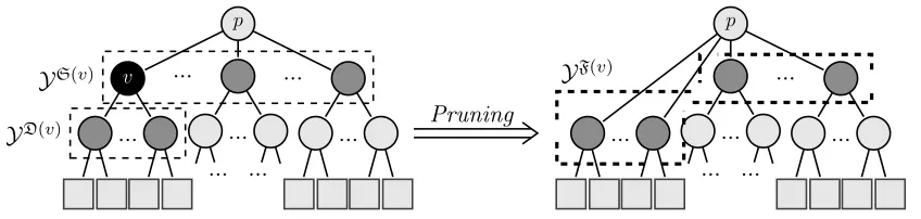
In this section, we present a strategy aiming at adapting the given hierarchy of classes by pruning some nodes in the hierarchy. An example of node pruning is shown in Figure 2. The rationale and motivation behind adapting the given hierarchyH= (V, E) to the set of input/output pair (x, y) is that
• Large-scale taxonomies, such as DMOZ and Yahoo! Directory, are designed with an intent of better user-experience and navigability, and not necessarily for the goal of classification,
• Taxonomy design is subject to certain degree of arbitrariness based on personal choices and preferences of the editors. Therefore, many competing taxonomies may exist, and
• The large-scale nature of such taxonomies poses difficulties in manually designing good taxonomies for classification.
... ... Pruning
Figure 2: The pruning procedure; the node in black is replaced by its children. In the figure on the left, the gray nodes represent the siblings or sisters of node in black.
on which we will develop a greedy procedure to simplify a given hierarchy. The rationale for a greedy approach here is that optimal pruning would require evaluations of 2k possible
prunings fork siblings, which is infeasible in practice.
4.1 Hierarchy Pruning based on validation estimate
The challenge in the pruning procedure is to identify promising nodes which when pruned lead to improvement in classification accuracy. One of the simplest methods to identify such nodes is by using a validation set to check if pruning a node improves classification accuracy on that set by comparing it with accuracy obtained on the original taxonomy. This can also be interpreted as follows:
Whether to prune a nodev? =
Yes If classification improves on the validation set No otherwise
Algorithm 1 Hierarchy pruning based on validation estimate
Require: A hierarchyG, Training set S and a validation set S0
1: Train SVM classifier at each node of the treeG using the training setS 2: Evaluate the accuracy of the classifier-cascadeG on the validation set
3: forv∈ V do
4: Prune the node v and replace it by its children
5: Re-train SVM classifier at the impacted node of the tree G0
6: Evaluate the accuracy of the classifier-cascade G0 on the validation set 7: if Cross-validation accuracy is higher onG0 as compared toG then 8: Prune the nodev
9: else
10: Do not prune the nodev
11: end if 12: end for
13: return Pruned taxonomyG0
taxonomies. In section 6, we also present experimental results obtained by this pruning strategy vis-`a-vis other pruning methods presented later in this paper.
Computationally, this method requires (i) a trained cascade of top-down classifiers, (ii) for every pruned node, re-training the parent of the pruned node, and (iii) for every such node, evaluating the top-down performance on the validation set, which involves traversing the root-to-leaf path of classifier evaluation along the taxonomy. Furthermore, the steps (ii) and (iii) are to be repeated for every pruned node. Let Ctd−cas denotes the computational
complexity for training the cascade,Cv denotes the complexity for re-training of the parent node after pruning the nodev, andCvaldenotes the complexity of evaluating the validation
set. Let |V|p denote the number of pruned nodes, then the complexity of the Algorithm
1 is Ctd−cas+|V|p×(Cv+Cval). Due to the linear dependence on the number of pruned
nodes, it becomes computationally expensive to prune a reasonably large number of nodes and check if this would result in improvement in classification accuracy of the top-down cascade. Furthermore, this process does not amount to a learning-based method for pruning and hence needs to be employed from scratch for newer taxonomies, even though these taxonomies may have similar characteristics to those encountered already.
To summarize, though quite simple, the above pruning method has the following disad-vantages:
• This is a computationally expensive process to re-train the classifier at the pruned nodes and then test the performance on the validation set. As a result, this may not be applicable for large-scale taxonomies consisting of large number of internal nodes,
• This method does not amount to a learning-based strategy for pruning, and ignores data-dependent information available at the nodes of the taxonomy, and
• This process needs to be repeated for each taxonomy encountered, and information gained from taxonomy cannot be leveraged for newer taxonomies with similar char-acteristics.
We now turn to another method for taxonomy adaptation by pruning which is based on the generalization error analysis derived in Section 3.1. This method is computationally efficient compared to that presented in Algorithm 1 and only requires a cascade of top-down classifiers. Essentially, the criterion for pruning, which is related to the margin at each node, can be computed while training the top-down cascade. This corresponds to only the first step in Algorithm 1, and rest of the steps of evaluating on validation set are no longer required. Therefore, in terms of computational complexity, the method proposed in the next section has complexity of Ctd−cas.
4.2 Hierarchy Pruning based on generalization-error
of the bound as compared to that attained by using the original hierarchy. For a nodevwith parentπ(v), pruningv and replacing it by its children will increase the number of children of π(v) and hence the associated Rademacher complexity but will decrease the empirical error along that path from root to leaf. Therefore, we need to identify those nodes in the taxonomy for which increase in the Rademacher complexity is among the lowest so that a better trade-off between the two error terms is achieved than in the original hierarchy. For this purpose, we turn to the bound on the empirical Rademacher complexity of the function classGFB.
In the derivation of Theorem 1, the empirical Rademacher complexity was upper bounded as follows:
ˆ
Rm(GFB,S)≤ 2
mEσ
sup ||W||H≤B
X
(v,v0)∈V2,v0∈S(v)
kwv−wv0k H
X
i:c(f,x(i),y(i))=(v,v0) σiΦ(x(i))
H
(2)
From the above bound, we define a quantityC(v) for each nodev
C(v) = X
(v,v0)∈V2,v0∈S(v)
kwv−wv0k
H (3)
As one can note, the right hand side of the inequality (2) above provides an upper bound on ˆ
Rm(GFB,S) and one can meaningfully compare only the sibling nodes since these nodes have the same training set. Thus, the explicit computation of expectation Eσ(.) with respect to
the Rademacher random variables and the computation of the inner product in the feature space can be avoided. This motivates the definition of C(v) in equation (3), that can be efficiently and effectively computed from the training data, and that represents a distance of node v to its sibling nodes. It must be noted that C(v0), for a set of siblings {v0}, as computed using equation 3 is different for each nodev0.
C(v) is higher when wv is larger than wv0 (when measured in terms of L2-distance),
for all siblingsv0 of v, or when wv is far away fromwv0 (implying that the L2-norm of the
difference is large), or both. The first and last cases correspond to unbalanced classes, v
being the dominant class. In such cases, pruningv by replacing it by its children leads to a more balanced problem, less prone to classification errors. Furthermore, as children ofvare based on the features inv, most of them will likely be far away from the siblings ofv, and the pruning, even though increasing the Rademacher complexity term, will decrease the empirical error term and, likely, the generalization error. In the second case, pruningv will lead to children that will again be, very likely, far away from the siblings ofv. This pruning thus does not introduce confusion between categories and reduces the problem related to error propagations.
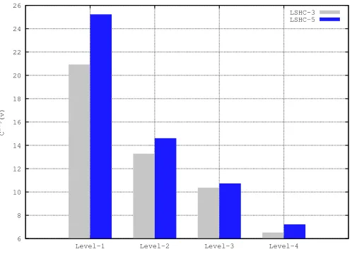
This suggests that an effective pruning algorithm must prune the nodes vin the taxon-omy for whichC(v) is maximal. In practice, we focus on pruning the nodes in the top-two layers of the taxonomy. This is due to the following reasons:
• The categories in these levels represent generic concepts, such as Entertainment and Sports in Yahoo! Directory, which are typically over-lapping in nature, and
• This is also shown in the plot in Figure 3 for the average confusion of the nodes Cvavg
that the confusion among the top-level nodes is much higher as compared to those in the lower levels.
6 8 10 12 14 16 18 20 22 24 26
Level-1 Level-2 Level-3 Level-4
C
avg
(v)
LSHC-3 LSHC-5
Figure 3: Cvavg plotted for various levels in the hierarchy Level 1 corresponds to
the top-most level.
Algorithm 2The proposed method for hierarchy pruning based on Generalization Bound
Require: a hierarchyG, Training setS consisting of (x, y) pairs, x∈ X and y∈ Y Train SVM classifier at each node of the tree
∆←0
for v∈ V do
Sort its child nodes v0 ∈D(v) in decreasing order of C(v0) Flatten 1st and 2nd ranked child nodes, sayv10 and v20 ∆=C(v01)−C(v20)
vprev←v20 . Set the previous flattened node tov02 forv0 ∈ V − {v10, v20},(v, v0)∈ E do
if C(vprev)−C(v0)< ∆then
Flattenv0
∆←C(vprev)−C(v0)
vprev←v0 . Set the previous flattened node tov0
else break end if end for end for
return Pruned taxonomy G0
The above criterion for pruning the nodes in a large-scale taxonomy is also similar in spirit to the method introduced by Babbar et al. (2013b) which is motivated from the generalization error analysis of Perceptron Decision Trees. As shown in the experiments on large-scale datasets by using SVM and Logistic Regression classifiers, applying this strategy outputs a new taxonomy which leads to better classification accuracy as compared to the original taxonomy.
It may be noted that the pruning procedure adopts a conservative approach to avoid excessive flattening of the taxonomy. It can be modified to prune the nodes more ag-gressively by scaling the parameter ∆after pruning of every node, and hence allow more nodes to be pruned. However, irrespective of such design choice, this method based on the generalization bound for pruning the hierarchy has two following disadvantages :
• Higher computational complexity since one needs to learn the weight vector wv for
each nodevin the given taxonomy. As a result, the process of identifying these nodes can be computationally expensive for large-scale taxonomies;
• It is restricted only to discriminative classifiers such as Support Vector Machines and Logistic Regression.
Therefore, we next present a meta-learning based pruning strategy for hierarchy prun-ing which avoids this initial trainprun-ing of the entire taxonomy, and is applicable to both discriminative and generative classifiers.
5. Meta-learning based pruning strategy
In this section, we present a meta-learning based generic pruning strategy which is applicable to both discriminative and generative classifiers. The meta-features for the instances are derived from the analysis of the approximation error for multi-class versions of the two well-known generative and discriminative classifiers: Naive Bayes and Logistic Regression. We then show how this generalization error analysis of the classifier at each node is combined when deployed in a typical top-down cascade of the hierarchy tree. Based on these analyses, we identify the important features that control the variation of the generalization error and determine whether a particular node should be flattened or not. We finally train a meta-classifier based on these meta-features, which predicts whether replacing a node in the hierarchy by its children (Figure 2) will improve the classification accuracy or not.
The remainder of this section is organized as follows:
1. In Section 5.1, we present asymptotic error bounds for Naive Bayes classifiers;
2. Asymptotic error bounds for Multinomial Logistic Regression classifiers are given in Section 5.2;
3. We then develop in Section 5.3:
(a) A pruningbound for both types of classifiers;
Theorem 2 below is recalled by Ng and Jordan (2001). Theorems 3 and 4 provide multi-class versions of the bounds proposed by Ng and Jordan (2001) for the Naive Bayes and Logistic Regression classifiers respectively. Lastly, Theorem 5 provides a hierarchical generalization of these bounds for both classifiers. The features we are using to learn the meta-classifier are derived from Theorem 5.
5.1 Asymptotic approximation error bounds for Naive Bayes
Let us first consider a multinomial, multiclass Naive Bayes classifier in which the predicted class is the one with maximum posterior probability. The parameters of this model are estimated by maximum likelihood and we assume here that Laplace smoothing is used to avoid null probabilities. Our goal here is to derive a generalization error bound for this classifier. To do so, we recall the bound for the binomial version (directly based on the presence/absence of each feature in each document) of the Naive Bayes classifier for two target classes (Theorem 4 of (Ng and Jordan, 2001)).
Theorem 2 For a two class classification problem in ddimensional feature space with m
training examples {(xi, yi)}im=1 sampled from distribution D, let h and h∞ denote the clas-sifiers learned from the training set of finite sizem and its asymptotic version respectively. Then, with high probability, the bound on misclassification error of h is given by
E(h)≤ E(h∞) +G O r
1
mlogd
!!
(4)
where G(τ) represents the probability that the asymptotic classifier predicts correctly and has scores lying in the interval (−dτ, dτ).
We extend here this result to the multinomial, multiclass Naive Bayes classifier, for aK
class classification problem withY ={y1, . . . yK}. To do so, we first introduce the following
lemma, that parallels Lemma 3 of (Ng and Jordan, 2001):
Lemma 1 ∀yk ∈ Y, let Pb(yk) be the estimated class probability and P(yk) its asymptotic version obtained with a training set of infinite size. Similarly,∀yk∈ Y and∀i, 1≤i≤d, let
b
P(wi|yk) be the estimated class conditional feature probability and P(wi|yk) its asymptotic
version (wi denotes the ith word of the vocabulary). Then, ∀ >0, with probability at least
(1−δ) we have :
|Pb(yk)−P(yk)|< , |Pb(wi|yk)−P(wi|yk)|<
withδ=Kδ0+dPkK=1δk, whereδ0 = 2 exp(−2m2)andδk= 2dexp(−2dk2). dkrepresents
the length of class yk, that is the sum of lengths (in number of occurrences) of all the
documents in class k.
The proof of this lemma directly derives from Hoeffding’s inequality and the union bound, and is a direct extension of the proof of Lemma 3 given by Ng and Jordan (2001).
Let us now denote the joint log-likelihood of the vector representation of (a document) x in classyk by l(x, yk) :
l(x, yk) = log
"
b
P(yk) d
Y
i=1 b
P(wi|yk)xi
#
where xi represents the number of times word wi appears inx. The decision of the Naive
Bayes classifier for an instance xis given by:
h(x) = argmax
yk∈Y
l(x, yk) (6)
and the one for its asymptotic version by:
h∞(x) = argmax
yk∈Y
l∞(x, yk) (7)
Lemma 1 suggests that the predicted and asymptotic log-likelihoods are close to each other, as the quantities they are based on are close to each other. Thus, provided that the asymp-totic log-likehoods between the best two classes, for any given x, are not too close to each other, the generalization error of the Naive Bayes classifier and the one of its asymptotic version are close to each other. Theorem 3 below states such a relationship, using the fol-lowing function that measures the confusion between the best two classes for the asymptotic Naive Bayes classifier.
Definition 1 Let l1∞(x) = maxyk∈Yl∞(x, yk) be the best log-likelihood score obtained for x
by the asymptotic Naive Bayes classifier, and let l2∞(x) = maxyk∈Y\h∞(x)l∞(x, yk) be the
second best log-likelihood score forx. We define the confusion of the asymptotic Naive Bayes classifier for a category set Y as:
GY(τ) =P(x,y)∼D(|l1∞(x)−l2∞(x)|<2τ) for τ >0.
We are now in position to formulate a relationship between the generalization error of the multinomial, multiclass Naive Bayes classifier and its asymptotic version.
Theorem 3 For a K class classification problem in d dimensional feature space with a training set of size m, {x(i), y(i)}m
i=1, x(i)∈ X, y(i)∈ Y, sampled from distribution D, let h and h∞ denote the Naive Bayes classifiers learned from a training set of finite size m and its asymptotic version respectively, and let E(h) and E(h∞) be their generalization errors. Then, ∀ >0, one has, with probability at least (1−δY):
E(h)≤ E(h∞) +GY() (8)
with:
δY = 2Kexp
−
22m
C(d+dmax)2
+ 2dexp
−
22dmin
C(d+dmax)2
where dmax (resp. dmin) represents the length (in number of occurrences) of the longest (resp. shortest) class in Y, and C is a constant related to the longest document in X.
ProofUsing Lemma 1 and a Taylor expansion of the log function, one gets,∀ >0,∀x∈ X, ∀k∈ Y:
P
|l(x, yk)−l∞(x, yk)|<
√
C
ρ0
where δ is the same as in Lemma 1, √C equals to the maximum length of a document and ρ0 = mini,k{P(yk), P(wi|yk)}. The use of Laplace smoothing is important for the
quantities p(wi|yk), which may be null if word wi is not observed in classyk. The Laplace
smoother in this case leads toρ0= d+d1
max. The log-likelihood functions of the multinomial, multiclass Naive Bayes classifier and the one of its asymptotic version are thus close to each other with high probability. The decision made by the trained Naive Bayes classifier and its asymptotic version on a givenxonly differ if the distance between the first two classes of the asymptotic classifier is less than two times the distance between the log-likelihood functions of the trained and asymptotic classifiers. Thus, using the union bound, one obtains, with probability at least (1−δ):
E(h)≤ E(h∞) +GY
√C(d+dmax)
Using a change of variable (0 =√C(d+dmax)) and approximating PK
k=1exp(−2dk2) by
exp(−2dmin2), the dominating term in the sum, leads to the desired result. 5.2 Asymptotic approximation error bounds for Multinomial Logistic
Regression
We now propose an asymptotic approximation error bound for a multiclass logistic regres-sion (MLR) classifier. We first consider the flat, multiclass case (V =Y), and then show how the bounds can be combined in a typical top-down cascade, leading to the identification of important features that control the variation of these bounds.
Considering a pivot class y? ∈ Y, a MLR classifier, with parameters β = {β0y, βjy;y ∈ Y \ {y?}, j ∈ {1, . . . , d}}, models the class posterior probabilities via a linear function in
x= (xj)dj=1 ((see for example Hastie et al., 2001, p. 96)) :
P(y|x;β)y6=y? =
exp(β0y+Pd
j=1β
y jxj)
1 +P
y0∈Y,y06=y?exp(βy 0
0 + Pd
j=1β
y0 j xj)
P(y?|x;β) = 1
1 +P
y0∈Y,y06=y?exp(β y0
0 + Pd
j=1β
y0 j xj)
The parameters βare usually fit by maximum likelihood over a training set S of sizem
(denoted byβbmin the following) and the decision rule for this classifier consists in choosing
the class with the highest class posterior probability :
hm(x) = argmax
y∈Y
P(y|x,βbm) (9)
The following lemma states to which extent the posterior probabilities with maximum like-lihood estimates βbm may deviate from their asymptotic values obtained with maximum
likelihood estimates when the training sizem tends to infinity (denoted byβb∞).
such that ∀y∈ Y\{y?},exp(β0y+Pd
j=1β
y jxj)<
√
R; then for all1> δ >0, with probability at least (1−δ) we have:
∀y∈ Y,
P(y|x,βbm)−P(y|x,βb∞) < d
r
R|Y|σ0
δm
where σ0 = maxj,yσyj and(σ y
j)y,j represent the components of the inverse (diagonal) Fisher
information matrix atβb∞ and are different from σi used in Section 3 wherein these repre-sented Rademacher random variables.
Proof By denoting the sets of parameters βbm = {βˆjy;j ∈ {0, . . . , d}, y ∈ Y \ {y?}}, and
b
β∞ = {βjy;j ∈ {0, . . . , d}, y ∈ Y \{y?}}, and using the independence assumption and the
asymptotic normality of maximum likelihood estimates ((see for example Schervish, 1995, p. 421)), we have, for 0 ≤ j ≤ d and ∀y ∈ Y \ {y?}: √m(βb
y
j −β
y
j) ∼ N(0, σ y
j) where
the (σjy)y,i represent the components of the inverse (diagonal) Fisher information matrix
at βb∞. Let σ0 = maxj,yσ
y
j. Then using Chebyshev’s inequality, for 0 ≤ j ≤ d and
∀y ∈ Y \ {y?} we have with probability at least 1−σ0/2, |βb
y
j −β
y
j| < √m. Further ∀x
and∀y ∈ Y\{y?},exp(β0y+Pd
j=1β
y jxj)<
√
R; using a Taylor development of the functions exp(x+) and (1 +x+x)−1 and the union bound, one obtains that, ∀ > 0 and y ∈ Y
with probability at least 1−|Y|σ0
2 :
P(y|x,βbm)−P(y|x,βb∞) < d
q
R
m. Setting
|Y|σ0
2 toδ, and solving for gives the result.
Lemma 2 suggests that the predicted and asymptotic posterior probabilities are close to each other, as the quantities they are based on are close to each other. Thus, provided that the asymptotic posterior probabilities between the best two classes, for any given x, are not too close to each other, the generalization error of the MLR classifier and the one of its asymptotic version should be similar. Theorem 4 below states such a relationship, using the following function that measures the confusion between the best two classes for the asymptoticMLR classifier defined as :
h∞(x) = argmax
y∈Y
P(y|x,βb∞) (10)
For any givenx∈ X, the confusion between the best two classes is defined as follows.
Definition 2 Let f∞1(x) = maxy∈YP(y|x,βb∞) be the best class posterior probability for x by the asymptotic MLR classifier, and let f∞2(x) = maxy∈Y\h∞(x)P(y|x,βb∞) be the second best class posterior probability forx. We define the confusion of the asymptoticMLRclassifier for a category set Y as:
GY(τ) =P(x,y)∼D(|f∞1 (x)−f∞2 (x)|<2τ) for a given τ >0.
The following theorem states a relationship between the generalization error of a trained
Theorem 4 For a multi-class classification problem ind dimensional feature space with a training set of size m, {x(i), y(i)}m
i=1, x(i) ∈ X, y(i) ∈ Y, sampled i.i.d. from a probability distribution D, let hm and h∞ denote the multiclass logistic regression classifiers learned from a training set of finite size m and its asymptotic version respectively, and let E(hm)
and E(h∞) be their generalization errors. Then, for all1 > δ >0, with probability at least
(1−δ) we have:
E(hm)≤ E(h∞) +GY d r
R|Y|σ0
δm
!
(11)
where √R is a bound on the function exp(β0y+Pd
j=1β
y
jxj),∀x∈ X and ∀y∈ Y, andσ0 is a constant.
ProofThe differenceE(hm)−E(h∞) is bounded by the probability that the asymptoticMLR
classifier h∞ correctly classifies an example (x, y)∈ X × Y randomly chosen fromD, while
hm misclassifies it. Using Lemma 2, for all δ ∈(0,1),∀x∈ X,∀y ∈ Y, with probability at least 1−δ, we have:
P(y|x,βbm)−P(y|x,βb∞) < d
r
R|Y|σ0
δm
Thus, the decision made by the trained MLR and its asymptotic version on an example (x, y) differs only if the distance between the two predicted classes of the asymptotic classifier is less than two times the distance between the posterior probabilities obtained with βbm and
b
β∞ on that example; and the probability of this is exactly GY
d
q
R|Y|σ0
δm
, which
upper-bounds E(hm)− E(h∞).
Note that the quantity σ0 in Theorem 4 represents the largest value of the inverse
(di-agonal) Fisher information matrix ((Schervish, 1995)), and thus corresponds to the inverse of the smallest value of the (diagonal) Fisher information matrix, which corresponds to the smallest amount of information one has on the estimation of each parameter βbjk. This
smallest amount of information is in turn related to the length (in number of occurrences) of the longest (resp. shortest) class in Y denoted respectively by dmax and dmin as, the smaller they are, the larger σ0 is likely to be.
5.3 A learning based node pruning strategy
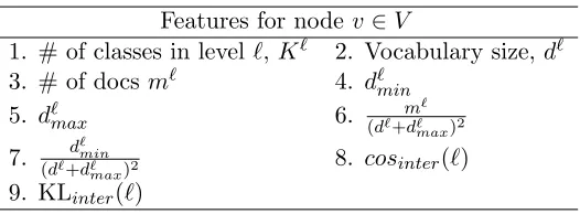
Let us now consider a hierarchy of classes and a top-down classifier making decisions at each level of the hierarchy. A node-based pruning strategy can be easily derived from the approximation bounds above. Indeed, any nodevin the hierarchyH= (V, E) is associated with three category sets: its sibling categories with the node itself S0(v) = S(v)∪ {v}, its children categories, D(v), and the union of its siblings and children categories, denoted F(v) =S(v)∪D(v).
These three sets of categories are the ones involved before and after the pruning of node
v. Let us now denote by hS0v
m a classifier learned from a set of sibling categories of node v
and the node itself, and by hDv
m a classifier learned from the set of children categories of
nodev(hS 0 v
∞ andhD∞v respectively denote their asymptotic versions). The following theorem
p
v
...
... ...
... ...
... ...
p
...
...
... ...
... ...
Pruning
YS(v)
YD(v)
YF(v)
Figure 4: The pruning procedure for a candidate class node u (in black). After replacing the candidate node by its children, the new category setYF(v)contains the classes
from both the daughter and the sister category sets ofv.
Theorem 5 Using notations from both Theorems 3 and 4, ∀ >0, v∈V \ Y, one has:
E(hS0v
m ) +E(hDmv)≤ E(hS 0 v
∞) +E(hD∞v) +GS0(v)() +GD(v)()
with probability at least 1−
Rd2|S0(v)|σS 0(v)
0
mS0(v)2 +
Rd2|D(v)|σ0D(v)
mD(v)2
for MLR classifiers and with
probability at least 1− δS0(v)+δD(v) for Naive Bayes classifiers, withδY defined in
The-orem 3.
{|Y`|, m
Y`, σY `
0 , d`max, d`min;Y` ∈ {S0(v),D(v)};} are constants related to the set of
cate-gories Y` ∈ {S0(v),D(v)} and involved in the respective bounds stated in Theorem 3 and
4. Denoting byhFv
m the classifier trained on the setF(v) and by hF∞v its asymptotic version,
Theorem 5 suggests that one should prune nodev if:
GF(v)()≤GS0(v)() +GD(v)() (12a)
and, forMLR classifiers:
|F(v)|σF0(v) mF(v)
≤ |S
0(v)|σS0(v) 0
mS0(v) +
|D(v)|σ0D(v) mD(v)
(12b)
or, for Naive Bayes classifiers:
δF(v)≤δS0(v)+δD(v) (12c)
The above conditions for pruning a node v rely on the union bound and thus are not likely to be exploitable in practice. They nevertheless exhibit the factors that play an important role in assessing whether a particular trained classifier is close or not to its asymptotic version. Following Definitions 1 and 2, GY() is of the form:
GY() =P(x,y)∼D(|g∞(x)−g∞(x)|<2)
Features for nodev∈V
1. # of classes in level`,K` 2. Vocabulary size, d`
3. # of docsm` 4. d`min
5. d`max 6. (d`+md`` max)2 7. d`min
(d`+d`
max)2 8. cosinter(`)
9. KLinter(`)
Table 1: Features involved in the vector representation of a node v ∈ H = (V, E). As
`∈ {F(v),D(v),S(v)}, we have in total 27 features associated with the different category sets considered for flattening nodeu.
between categories and can thus be approximated by measures of the similarity between classes. We propose here to estimate this confusion with two simple quantities: the average cosine similarity of all the pairs of classes in Y, and the average symmetric Kullback-Leibler divergences between all the pairs in Y according to class conditional multinomial distributions. Each node v ∈ V when deployed with MLR and Naive Bayes classifiers can then be characterized by factors shown in Table 1, which are involved in the estimation of inequality (12) above.
The average cosine similarity and the average symmetric KL divergence are calculated as follows for each pair of nodes (u, v) in levell:
cosinter(`) = 1
K`
X
k=1
K`
X
k0=1k06=k
mu`
kmvk`0 K`
X
k=1
K`
X
k0=1k06=k
mu`
kmv ` k0cos(u
` k, v`k0)
KLinter(`) =
1
K`(K`−1)
K`
X
k=1
K`
X
k0=1k06=k
KL(Qu`
k||Qvk`0
) +KL(Qv` k0
||Qu` k),
where KL(Qu||Qv) denotes the Kullback-Leibler divergence between the class conditional
probability distributions of the features present in the two classes u and v:
KL(Qu||Qv) =
X
w∈u,v
p(w|u) logp(w|u)
p(w|v)
where p(w|u) denotes the probability of word/feature w in class u, taking smoothing into account.
Algorithm 3 The pruning strategy.
1: procedure Prune Hierarchy(a hierarchyH, a meta-classifierCm)
2: clist[]←H.root; . Initialize with root node
3: while !clist.isEmpty()do
4: parent←clist.getN ext()
5: list[]←Ch(parent); . Candidate children to merge
6: while!list.isEmpty() do
7: index← MERGE(parent,list,Cm); . Index of children to be merged
8: if index==−1 then
9: break;
10: end if
11: list.add(Ch(list[index])) . Move up the children of node list[index]
12: list.remove(index); .This node has been merged
13: end while
14: clist.add(Ch(clist[j])); . Adds next level parents
15: end while
16: export new hierarchy;
17: end procedure
nodes should be pruned. A simple strategy to adopt is then to prune nodes in sequence: starting from the root node, the algorithm checks which children of a given nodev should be pruned (lines 6-13) by creating the corresponding instance and feeding the meta-classifier; the child that maximizes the probability of the positive class is then pruned; as the set of categories has changed, we recalculate which children ofv can be pruned, prune the best one (as above) and iterate this process till no more children of v can be pruned; we then proceed to the children of v and repeat the process. The function MERGE takes as arguments the parent, the candidate children to be merged as well as the meta-classifier. It returns the index of the child that should be merged. In case where the meta-classifier does not identify any child eligible for merging then the pruning procedure continues with the next parent in the list. The meta-classifier tries to predict whether pruning a specific node will lead to an increase of the performance over 10%. That means that the classifier may identify several candidate nodes and one of them will be selected for pruning.
6. Experimental Analysis
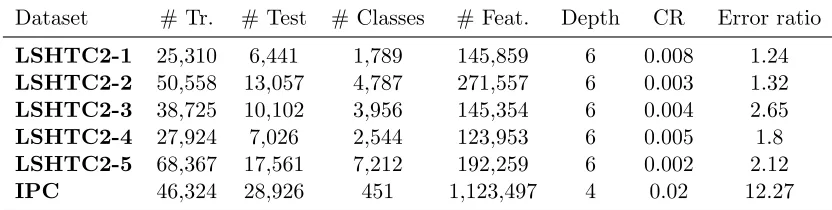
We start our discussion by presenting results on different hierarchical datasets with different characteristics usingMLRand SVMclassifiers. The datasets we used in these experiments are two large datasets extracted from the International Patent Classification (IPC) dataset3 and the publicly available DMOZ dataset from the second LSHTC challenge (LSHTC2)4. Both datasets are multi-class;IPCis single-label andLSHTC2multi-label with an average of 1.02 categories per class. We created 5 datasets from LSHTC2by splitting randomly the first layer nodes (11 in total) of the original hierarchy in disjoint subsets. The classes
3.http://www.wipo.int/classifications/ipc/en/support/
Dataset # Tr. # Test # Classes # Feat. Depth CR Error ratio
LSHTC2-1 25,310 6,441 1,789 145,859 6 0.008 1.24
LSHTC2-2 50,558 13,057 4,787 271,557 6 0.003 1.32
LSHTC2-3 38,725 10,102 3,956 145,354 6 0.004 2.65
LSHTC2-4 27,924 7,026 2,544 123,953 6 0.005 1.8
LSHTC2-5 68,367 17,561 7,212 192,259 6 0.002 2.12
IPC 46,324 28,926 451 1,123,497 4 0.02 12.27
Table 2: Datasets used in our experiments along with the properties: number of train-ing examples, test examples, classes and the size of the feature space, the depth of the hierarchy and the complexity ratio of hierarchical over the flat case (P
v∈V\Y|D(v)|(|D(v)| −1)/|Y|(|Y| −1)), the ratio of empirical error for
hierar-chical and flat models.
for the IPC and LSHTC2datasets are organized in a hierarchy in which the documents are assigned to the leaf categories only. Table 2 presents the characteristics of the datasets. CR denotes the complexity ratio between hierarchical and flat classification, given by the Rademacher complexity term in Theorem 1: P
v∈V\Y|D(v)|(|D(v)| −1)
/(|Y|(|Y| −1)); the same constantsB,R andLare used in the two cases. As one can note, this complexity ratio always goes in favor of the hierarchical strategy, although it is 2 to 10 times higher on the IPC dataset, compared to LSHTC2-1,2,3,4,5. On the other hand, the ratio of empirical errors (last column of Table 2) obtained with top-down hierarchical classification over flat classification when using SVM with a linear kernel is this time higher than 1, suggesting the opposite conclusion. The error ratio is furthermore really important onIPC
compared to LSHTC2-1,2,3,4,5. The comparison of the complexity and error ratios on all the datasets thus suggests that the flat classification strategy may be preferred onIPC, whereas the hierarchical one is more likely to be efficient on theLSHTC datasets. This is indeed the case, as is shown below.
To test our simple node pruning strategy, we learned binary classifiers aiming at deciding whether to prune a node, based on the node features described in the previous section. The label associated to each node in this training set is defined as +1 if pruning the node increases the accuracy of the hierarchical classifier by at least 0.1, and -1 if pruning the node decreases the accuracy by more than 0.1. The threshold at 0.1 is used to avoid too much noise in the training set. The meta-classifier is then trained to learn a mapping from the vector representation of a node (based on the above features) and the labels{+1;−1}. We used the first two datasets of LSHTC2to extract the training data whileLSHTC2-3,
4,5 and IPCwere employed for testing.
of trees ({10, 20, 50, 100 and 200}), the depth of the trees ({unrestricted, 5, 10, 15, 30, 60}), as well as the number of iterations in AdaBoost ({10, 20, 30}). The final values were selected by cross-validation on the training set (LSHTC2-1and LSHTC2-2) as the ones that maximized accuracy and minimized false-positive rate in order to prevent degradation of accuracy. For example, Table 6 presents the true positive and false positive rates for the two classes for the meta-dataset of MLR.
Class TP rate FP rate
Prune (+1) 0.737 0.020
Do not prune (-1) 0.980 0.263
Table 3: True positive and false positive rates for the MLRmeta-daset (119 examples).
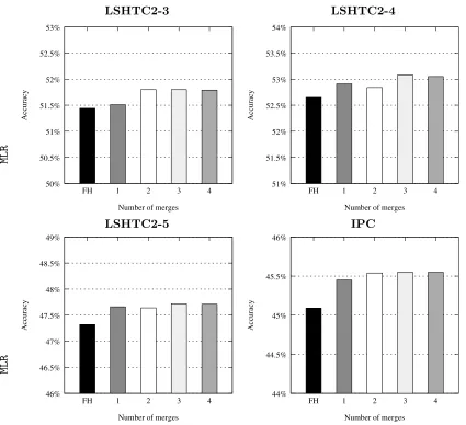
We consider three different classifiers which include Multinomial Naive Bayes (MNB), Multi-class Logistic Regression (MLR) and Support Vector Machine (SVM) classifiers. The configurations of the taxonomy that we consider are fully flat classifier (FL), fully hierar-chical (FH) top-down Pachinko machine, a random pruning (RN), and the two proposed pruning methods which include (i) Bound-based pruning strategy (PR-B) given in Section 4 and (ii) Meta-learning based pruning strategy (PR-M) proposed in Algorithm 3. For the PR-M pruning method, our experimental setup involves two scenarios: (i) The meta-classifier is trained over one kind of DMOZ hierarchy (LSHTC2-1, and LSHTC-2) and tested over another DMOZ hierarchy (LSHTC-3, LSHTC-4 and LSHTC-5), such that both sets have similar characteristics, and secondly, (ii) The meta-classifier is trained over one set of DMOZ hierarchy (LSHTC2-1, and LSHTC-2) and tested over IPC hierarchy which is derived from a different domain (patent classification) such that both sets have much less common characteristics. In this sense, our meta-classifier could learn to learn over one doamin and apply the learnt knowledge to another domain. For the random pruning we restrict the procedure to the first two levels and perform randomly prune 4 nodes (this is the average number of nodes that are pruned in the PR-M and PR-B strategies). We also present results for another pruning strategy proposed in our earlier work (Babbar et al., 2013b) which is based on error analysis of Perceptron Decision Trees (Bennett et al., 2000), and is referred to as PR-P. The results for the naive pruning method based on estimate on a validation set (as described in Section 4.1) are also presented, and referred to as PR-V. For each dataset we perform 5 independent runs for the random pruning and we record the best performance. For MLR and SVM, we use the LibLinear library (Fan et al., 2008) and use squared hinge-loss with L2-regularized versions, setting the penalty parameter C by cross-validation.
6.1 Flat versus Hierarchical classification
LSHTC2-3 LSHTC2-4 LSHTC2-5 IPC
MNB MLR SVM MNB MLR SVM MNB MLR SVM MNB MLR SVM
FL 73.0↓↓ 52.8↓↓ 53.5↓↓ 84.9↓↓ 49.7↓↓ 50.1↓↓ 83.9↓↓ 54.2↓↓ 54.7↓↓ 67.2↓↓ 54.6 46.6
RN 61.9↓↓ 49.3↓↓ 51.7↓↓ 70.5↓↓ 47.8↓↓ 48.4↓↓ 69.0↓↓ 53.2↓↓ 53.6↓ 64.3↓↓ 54.7↓ 50.2↓↓ FH 62.0↓↓ 48.4↓↓ 49.8↓↓ 68.3↓ 47.3↓↓ 47.6↓ 65.6↓ 52.6↓ 52.7 64.4↓ 55.2↓ 51.3↓↓ PR-V 61.7 48.2 49.5 65.9 46.7 46.6 67.7 52.3 52.2 63.7 54.6 50.3
PR-B - 48.1 49.5 - 46.6 46.5 - 52.2 52.2 - 54.5 50.5
PR-M 61.3 48.0 49.3 65.4 46.9 47.2 67.8 52.2 52.3 63.9 54.4 50.7
PR-P - 48.3 49.6 - 46.6 46.8 - 52.4 52.3 - 54.5 50.9
Table 4: Error results across all datasets. Bold typeface is used for the best results. Sta-tistical significance (using micro sign test (s-test) as proposed in (Yang and Liu, 1999)) is denoted with↓ for p-value<0.05 and with ↓↓ for p-value<0.01.
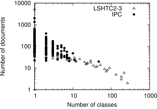
1 10 100 1000 10000
1 10 100 1000
Number of documents
Number of classes LSHTC2-3
IPC
Figure 5: Number of classes (on X-axis) which have the specified number of documents (on Y-axis) forLSHTC2-3 dataset andIPCdataset
of taxonomies. Further, the work by Liu et al. (2005) demonstrated that class hierarchies on LSHTCdatasets suffer from rare categories problem, i.e., 80% of the target categories in such hierarchies have less than 5 documents assigned to them. The value for Macro-F1 measure which weighs all leaf-level classes equally (in contrast to Micro-F1 which weighs each example in the test set equally) is given in Table 5. Macro-F1 measure is particularly interesting when dealing with datasets consisting of rare-categories, which is typically the case in most naturally occurring category systems such as DMOZ and Wikipedia.