On the Solution of a Optimal Control Problem for a Hyperbolic System

(1)

http://www.sciencepublishinggroup.com/j/acm doi: 10.11648/j.acm.20180703.11

ISSN: 2328-5605 (Print); ISSN: 2328-5613 (Online)

On the Solution of a Optimal Control Problem for a

Hyperbolic System

Fatma Toyoğlu

Department of Mathematics, Faculty of Art and Science, Erzincan University, Erzincan, Turkey

Email address:

To cite this article:

Fatma Toyoğlu. On the Solution of a Optimal Control Problem for a Hyperbolic System. Applied and Computational Mathematics. Vol. 7, No. 3, 2018, pp. 75-82. doi: 10.11648/j.acm.20180703.11

Received: April 24, 2018; Accepted: May 10, 2018; Published: May 25, 2018

Abstract:

In this study, the problem of determining the control function that is at the right hand side of a hyperbolic system from the final observation is investigated. Using the Fourier-Galerkin method, the weak solution of this hyperbolic system is obtained. The necessary conditions for the existence and uniqueness of the optimal solution are proved. We also find the approximate solutions of the test problems in numerical examples by a MAPLE® program. Finally, the numerical results are presented in the form of tables.

Keywords:

Optimal Control, Partial Differential Equation, Numerical Approximation

1. Introduction

The problem of determining the control function that is at the right hand side of the hyperbolic system has been studied by different authors. Lions [3] examined the problems in detail when the control function is at the right hand side of the hyperbolic problem by using different cost function. Periago [4] has investigated the problem of optimizing the shape and position of the support of the internal exact control of minimal 0, norm for the 1-D wave equation.

Yamamoto [5] has studied the inverse problem of determining from subject to the hyperbolic problem

, ∆ , , ∈ Ω, 0

, 0 0, , 0 0, ∈ Ω

, 0, ∈ Ω, 0

where ∈ 0, .

Benamou [6] has used the domain decomposition method to solve the optimal control problem in the hyperbolic system and has taken the set of admissible control as a convex subset of 0, Ω .

Kim and Pavol [7] have minimized the cost functional

! ! "#$) , % &$ , %' (

* (

+

*

governed by periodic nonlinear 1-D wave equation. The necessary and sufficient conditions for an admissible pair

∗_,∗ _∈ - _ℚ - _{ℚ , ℚ} _{0, /} _0, _{to be an}

optimal pair have given by authors.

Lopez at all. [8] have considered problem of controlling the function , related to the hyperbolic problem

0 11 ∆ 1 13 , ∈ Ω 0,

, 0 * _,

1 , 0 , ∈ Ω

, 0, , ∈ Ω 0, .

Privat et al. [9] have minimized the norm of the control for given initial data in the wave equation defined on 0, / with Homogeneous Dirichlet boundary condition when the control is in at the right hand side of the equation.

Subaşı and Saraç [10] have obtained a minimizer function for the optimal control problem of the initial velocity in a wave equation.

Saraç and Şener [11] have determined the transverse distributed load in Euler-Bernoulli beam problem from of admissible control. The set of admissible controls has been taken as a subspace of the space 56, 78.

(2)

using the initial velocity as a control function in hyperbolic problem.

Şener et al. [14] have explained applications of the Galerkin method to wave equation.

The problem of determining of unknown spatial load distributions in a vibrating Euler–Bernoulli beam from limited measured data has been solved in [16].

The space 0, consist of the functional which are square integrable, inner product and norm in 0, are defined respectively as;

, 9: = ; ( <

* and ‖ ‖9: = > , 9:.

Let ?_@A be closed, convex subset of 0, .

In this study, we consider an optimal control problem for a wave equation with homogeneous Dirichlet boundary conditions, the control being the one from the functions that

are at the right hand side of the equation. We determining the unknown function in the closed and convex subset

?@A⊂ 0, from the target , ; , which correspond

to final position using −norm. We are interested in generating Maple® procedure easy to used for obtaining approximate optimal control. The useful approximate optimal control function is easily obtained in some numeric examples.

We consider the following final optimal control problem: Choose a control ∈ 0, and a corresponding such that the pair , minimizes the functional

D = ‖ , ; − E ‖9:*,< + F‖ ‖9:*,< (1)

subject to the hyperbolic problem;

11− 6 GG= , , ∈ Ω ≔ 0, × 0, 8

, 0 = I , 1 , 0 = J , ∈ 0,

0, = 0, , = 0, ∈ 0, 8.

(2)

where E is given target function and I, J and are known functions.

With the choice of the functional in (1), we mentioned the observation of , ; in 0, for the control ∈

0, . Our aim is to obtain suitable function ∗ which approaches the solution of the problem (2) to desired target

E ∈ 0, at the final time = . Another word, we want to find the function ∗∈ ?_@A such that

Inf _D = _D ∗ .

Here F > 0 is a regularization parameter which ensures both the uniqueness of the solution and a balance between the norms ‖ , ; − E ‖₉_:_*,< and ‖ ‖₉_:_*,< . Detailed information as regards the regularization parameter can be found in [2]. The term ‖ ‖ ₉_: is called penalization term; its role is to avoid using too large controls in the minimization of _D .

In system (2), the term is considered to be an external force. External forces in this form of separation of variables are important in modelling vibrations. In [5] Yamamoto point out that the system (2) is regarded as

approximation to a model for elastic waves from a point dislocation source.

This paper is organized as follows. In section 2, we state the definition for solution of the wave equation considered and give the necessary conditions for the existence and uniqueness of the optimal solution. In section 3, we give Frechet derivative of the cost functional and construct a minimizing sequence that converge to the optimal solution. In the last section, we obtain the approximate solutions on numeric examples.

2. Existence of Unique Optimal Solution

In this section, we give the solvability of the optimal control problem (1)-(2). First we state the generalized solution of the hyperbolic problem (2) in view of [1].

Definition 2.1. The generalized (weak) solution of the problem (2) will be defined as the function ∈ K_* Ω , with

, 0 = I , ∈ 0, which satisfies the following integral identity:

; ; −_*+ _*< 1L1+ 6 GLG ( ( = ; ; L( (_*+ _*< + ; JL , 0_*< ( (3)

for all L ∈ K_* Ω with L , = 0. To have this solution the followings are needed;

∈ 0, , ∈ 0, , I ∈ K* 0, , J ∈ 0, (4) Theorem 2.2. Suppose that the condition (4) holds, then the problem (2) has a unique generalized solution and the following estimate is valid for this solution;

‖ ‖_K 0

1_Ω ≤ N* ‖I‖_K 0

1_0,l + ‖

J

‖ ₂_0, + Q Q ₂_0, ‖

‖ ₂_0, (5)

Proof of this theorem can easily be obtained by Galerkin method used in [1].

Let’s give the increment ∆ to such that + ∆ ∈ ?_@A

and show the solution of (2) corresponding + ∆ by

(3)

∆ 11= 6 ∆ GG+ ∆

∆ , 0 = 0, ∆ 1 , 0 = 0 (6) ∆ 0, = 0, ∆ , = 0

Lemma 2.3: Let ∆ be the solution of the problem (6). Then the following estimate is valid:

‖∆ , ‖ ₂_0, ≤ N ‖∆ ‖ ₂_0, (7)

Proof: We can proof this lemma in view of [15]. We multiply both sides of the hyperbolic equation (6) by ∆ ₁, then integrate it on 50, 8. After some transformations, we have

1

2( R! 5 ∆( 1 + 6 ∆ G 8( <

* S = ! ∆ ∆ 1 , ; (

<

* + 6 ∆ G∆ 1 |GU*

GU<_.

Using here the homogeneous boundary conditions of the system (6), we get

1

2( R! 5 ∆( 1 + 6 ∆ G 8( <

* S = ! ∆ ∆ 1 , ; (

<

* .

Integrating both sides on 50, 8, ∈ 50, 8, we get

V = ! ! W ∆ ∆ 1 , W; ( <

* (W

1

* , ∀ ∈ 50, 8

where

V =1_{2 ! 5 ∆} 1 + 6 ∆ G 8( <

* , ∈ 50, 8

We differentiate both the sides

2V V = ! ∆ ∆ 1 , ; (

<

* , ∀ ∈ 50, 8.

Appling to the right-hand side the Cauchy inequality, we obtain

2V V ≤ ‖∆ ‖9:*,< ‖∆ 1‖9: *,<, ∀ ∈ 50, 8.

Since we have

‖∆ 1‖9:*,< ≤ ! 5 ∆ 1 + 6 ∆ G 8( <

* = 2V , ∀ ∈ 50, 8

we get

V ≤ 1

√2 ‖∆ ‖9: *,<, ∀ ∈ 50, 8.

Integrating both the sides on 50, 8, ∈ 50, 8 and taking into account V 0 = 0, we obtain

V ≤ 1

√2‖∆ ‖9:*,< ! W (W 1

* , ∀ ∈ 50, 8.

Substituting in last inequality = , we write

V ≤

√2‖∆ ‖9:*,<

(4)

! 5∆< , 8 (

* = ! Z! ∆ 1 , (

+

* [ (

<

* ≤ ! ! 5∆ 1 , 8 ( (

+

* <

*

≤ 2 ! V+ (

* .

Combining last inequalities, we get

! 5∆< , 8 (

* ≤ 2 ! 2 ‖∆ ‖9:*,<( +

* ≤ ‖∆ ‖9:*,<

which implies the required estimate (7).

We can write the cost functional (1) in the following way;

D = !5 , ; − , ; 0 + , ; 0 − E 8 <

*

( + F ! <

* (

So we rewrite _D as

D = / , − 2 + 7 (8)

for

/ , = ; 5_*< , ; − , ; 0 8 ( + F ; _*< ( (9)

= ; 5_*< , ; − , ; 0 85E − , ; 0 8( (10)

and

7 = ; 5E_*< − , ; 0 8 ( (11)

Due to the linearity of the transform → 5 8 − 508, it can easily be seen that the functional / , is bilinear and symmetric. Further, we write the following;

| / , | ≥ F‖ ‖9:*,< (12)

and this implies the coercivity of / , . Since

/ , L = !5 , ; − , ; 0 8 <

*

5 , ; L − , ; 0 8( + F ! L( <

*

applying Cauchy-Schwartz inequality and using (7), we get

|/ , L | ≤ N ‖ ‖ ₂0, ‖L‖ 20, (13)

for N = ^6 _N , F`. Then / , L is continuous. The functional is linear. We can easily write that

≤ Na‖ ‖ ₂0, (14)

using (7). Hence we see that the functional is continuous. Theorem 2.4. Let / , be a continuous symmetric bilinear coercive form and be a continuous linear form. Then there exists a unique element ∗∈ ?_@A such that

D ∗ = Inf_{e ∈ f}

gh D .

Proof of this theorem can easily be obtained by showing the weak lower semi-continuity of _D same as in [3].

3. Frechet

Differential of the Cost

Functional and Minimizing Sequence

Let us introduce the Lagrangian , , i given by

(5)

Using the j = 0 stationarity condition, we get the following adjoint problem:

i11− 6 iGG= 0

i , = 0, i1 , = 25 , ; − E 8 i 0, = 0, i , = 0

(16)

Now, we investigate the variation of the functional _D . The difference functional

∆D = D + ∆ − D is such as

∆D = ; 52_*< , ; − 2E 8∆ , ( + ; 5∆_*< , 8 ( + F ; 2 + ∆ ∆ (_*< (17)

Here, the term

2 !5 , ; − E 8∆ , ( <

*

must be evaluated. Using the problems (6) and (16) we have

2 !5 , ; − E 8∆ , ( <

*

= − ! ! i , ∆

( (

0 0

So the relation (17) can be written as

∆D = ; k− ;_*< _*+ i , + 2F l ∆ ( + ; 5∆_*< , 8 ( + F ; ∆ (_*< . (18)

Using Lemma 2.3 in the (18), we can write the following equality:

∆D = 〈− ! i , ( +

*

+ 2F , ∆ 〉9:*,< + o ‖ ‖9:*,<

By the definition of Frechet differential at ∈ ?_@A we get the gradient

D = − ! i , ( +

*

+ 2F .

So, we can state the following theorem in view of [2].

Theorem 3.1. The control ∗ and the state ∗= ∗ are optimal if there exists a multiplier i∗∈ ?_@A such that i∗ and ∗ satisfy the following optimality conditions:

〈− ;+ i∗ _{, ( + 2F}∗_{, −}∗

* 〉 20, ≥ 0 (19)

for ∀ ∈ ?_@A.

Now, we can apply standard steepest descent iteration. We write an iterative procedure to compute a sequence of controls

_ p` convergent to the optimal one.

Select an initial control _*. If _p is known q ≥ 0 then _pr is computed according to the following scheme. 1. Solve the state problem (2) in the sense (3) and get corresponding _p.

2. Knowing _psolve the adjoint problem (16). 3. Using i_p get the gradient _{D p}

4. Set

pr = p− sp D p (20)

and select the relaxation parameter s_p in order to assure that

D pr − D p = spt−‖D p ‖ +u v_v_wwx < 0 (21)

for sufficiently small s_p > 0. The term o s_p is infinite decreasing term with high order respect to s_p. Computations of the s_p can be carried out by one of the methods shown in [13].

(6)

‖ pr − p‖ < 0 , | D pr − D p | < 0 , ‖D p ‖ < 0a. Lemma 3.2. The cost functional (1) is strongly convex with the strong convexity constant F. From the following strongly convex functional definition for z ∈ 50,18:

D z + 1 − z ≤ zD + 1 − z D − {z 1 − z ‖ − ‖9:*,<

we can see that cost functional (1) is strongly convex the constant { = F.

So, we can give the following theorem which states the convergence of the minimizer to optimal solution.

Theorem 3.3.Let ∗ be optimum solution of the problem (1)-(2). Then the minimizer given in (20) satisfies the following inequality;

‖ p− ∗‖ ≤_D$D p − D ∗ %, q = 0,1,2, … (22)

Proof of this theorem is obtained by taking z = in the definition of the above strongly convex functional.

4. Numerical Example

In this section we test the method in a numerical example. The used trigonometric basis functions are chosen such as;

}~2sin "/ ' , ~2sin •2/ ‚ , ~2sin •3/ ‚ , . . , ~2sin •„/ ‚…

for the generalized solution of the hyperbolic problem (2). Example 4. 1: Let us consider the following problem of minimizing the cost functional:

D = ! 5 , 1; 8 (

* + F ! (*

under the following condition:

11− GG= − 1 , , ∈ 0,2 × 0,18

, 0 = − †_{−7 + 19 − 10 1 ≤ ≤ 2}a+ 0 < ≤ 1

1 , 0 = †

a₊ _{0 < ≤ 1}

−7 + 19 − 10 1 ≤ ≤ 2 0, = 0, 2, = 0, ∈ 0,18.

The weak solution of this problem is

, = − 1 †_{−7 + 19 − 10 1 ≤ ≤ 2.}a+ 0 < ≤ 1

The function and its partial derivatives _G, ₁ belong to Ω . The function , is not a classical solution since _GG ∉ Ω . Here the force function is discontinuous.

Rewrite the functional as

D = D + FD

where

D = ! 5 , 1; 8 ( *

D = ! ( *

Choosing F = 0.1, starting the initial element _*= Š‹Œ/ and the relaxation parameter

sp = 0.1 assures the inequality *. pr < *. p .

We get the following approximate minimizing function and the values of the _*. _•• and _*. _•• , respectively;

••= −0.088086149 sin 3.14159265 − 1.66789652 sin 1.57079632 −0.011854776 sin 4.71238898 + 0.00127332 sin 6.28318530 −0.000781035 sin 7.85398163 − 0.00106163 sin 9.42477796 −0.000162151 sin 10.9955742 + 0.00003977 sin 12.5663706 −0.000042586 sin 14.1371669 − 0.00008255 sin 15.7079632

,

*. •• = 5.303067954,

*. •• = 2.789781915

(7)

Table 1. _{The values of functions and iteration numbers for different}F_{values of Example.}

“ ”“• –∗ ”“— –∗ ˜

0.9 5.880206210 0.0502480698 15

0.7 5.855965285 0.0801608045 18

0.5 5.812154139 0.1484081594 23

0.2 5.606363377 0.7782944222 47

0.08 5.148875247 4.2750794700 112

0.06 4.927442646 7.1645327120 147

0.05 4.764295988 9.8422178970 174

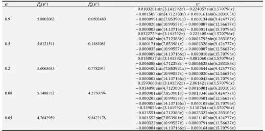
Table 2. _{The values of}_D ∗, _D ∗_{and the optimal controls} ∗_{for different}F_{values of Example.}

“ ”“• –∗ ”“— –∗ –∗

0.9 5.8802062 0.0502480

0.0183201 sin 3.141592 − 0.224057 sin 1.570796 −0.0015055 sin 4.712388 + 0.000161 sin 6.283185 −0.0000991 sin 7.853981 − 0.000134 sin 9.424777 −0.000020 sin 10.99557 + 0.0000087 sin 12.56637 −0.000005 sin 14.137166 − 0.000011 sin 15.70796

0.5 5.8121541 0.1484081

0.2 5.6063633 0.7782944

0.08 5.1488752 4.2750794

0.05 4.7642959 9.8422178

−0.339056 sin 3.141592 − 3.118764 sin 1.570796 −0.023551 sin 4.712388 + 0.0025322 sin 6.283185 −0.001552 sin 7.853981 − 0.0021105 sin 9.424777 −0.000322 sin 10.99557 + 0.0000791 sin 12.56637 −0.000084 sin 14.137166 − 0.000164 sin 15.70796

5. Conclusion

In this paper, we show that the external force in the wave equation be controlled by minimizing the distance between final situation distance and the desired target function. By using the adjoint approach in the mathematical analysis of the optimal control problem for wave equation, the gradient of the cost functional can be obtained. The minimizing sequence is constructed via this gradient.

References

[1] Ladyzhenskaya, O. A., Boundary Value Problems in Mathematical Physics, Springer, New York, 1985.

[2] Vasilyev, F. P., Numerical Methods for Solving Extremal Problems, Nauka, Moskow, 1988.

[3] Lions, J. L., Optimal Control of Systems Governed by Partial Differential Equations, Springer-Verlag, New York, 1971. [4] Periago, F., Optimal shape and position of the support for the

internal exact control of a string, Systems & Control Letters, 58, 136-140, 2009.

[5] Yamamoto, M., Stability, reconstruction formula and

regularization for an inverse source hyperbolic problem by a control method, Inverse Probl., 11, 481-496, 1995.

[6] Benamou, J. D., Domain Decomposition, “Optimal Control of Systems Governed by Partial Differential Equations, and Synthesis of Feedback Laws”, Journal Of Optimization Theory And Applications: Vol. 102. No. 1. 15-36, 1999. [7] Kim J., Pavol., N. H., Optimal control problem for the

periodic one-dimensional wave equation, Nonlinear Analysis Forum 3, 89-110, 1998.

[8] Lopez, A., Zhang, X., Zuazua, E., Null controllability of the heat equation as singular limit of the exact controllability of dissipative wave equations, J. Math. Pures. Appl., 79, 8, 741-808, 2000.

[9] Privat Y., Trelat., E., Zuazua, E., Optimal location of controllers for the one-dimensional wave equation, Annales de L’Institut Henri Poincare (C) Analyse Non Lineaire, 30, 1097-1126, 2013.

[10] Subaşı, M., and Saraç, Y., A Minimizer for Optimizing the Initial Velocity in a Wave Equation, Optimization, 61, 3, 327-333, 2012.

(8)

[12] Saraç, Y., “Symbolic and numeric computation of optimal initial velocity in a wave equation”, Journal of Computational and Nonlinear Dynamics, 8 (1), 2013.

[13] İskenderov, A. D., Tagiyev, R. Q. and Yagubov, Q. Y, Optimization Methods, Çaşıoğlu, Bakü, 2002.

[14] Şener, S. Ş, Saraç, Y and Subaşı, M, “Weak solutions to hyperbolic problems with inhomogeneous Dirichlet and Neumann boundary conditions”, Applied Mathematical Modelling, 37, pp. 2623-2629, 2013.

[15] Hasanov, A., “Simultaneous Determination of the Source Terms in a Linear Hyperbolic Problem from the Final Overdetermination: Weak Solution Approach,” IMA J. Appl. Math.,74, pp. 1-19, 2009.