Machine Learning in an Auction Environment
Patrick Hummel [email protected]
1600 Amphitheatre Parkway Google Inc.
Mountain View, CA 94043, USA
R. Preston McAfee [email protected]
One Microsoft Way Microsoft Corp.
Redmond, WA 98052, USA
Editor:Shie Mannor
Abstract
We consider a model of repeated online auctions in which an ad with an uncertain click-through rate faces a random distribution of competing bids in each auction and there is discounting of payoffs. We formulate the optimal solution to this explore/exploit problem as a dynamic programming problem and show that efficiency is maximized by making a bid for each advertiser equal to the advertiser’s expected value for the advertising opportunity plus a term proportional to the variance in this value divided by the number of impressions the advertiser has received thus far. We then use this result to illustrate that the value of incorporating active exploration in an auction environment is exceedingly small.
Keywords: Auctions, Explore/exploit, Machine learning, Online advertising
1. Introduction
In standard Internet auctions in which bidders bid by specifying how much they are willing to pay per click, it is standard to rank the advertisers by a product of their bid and their click-through rate, or their expected cost-per-1000-impressions (eCPM) bids. While this is a sensible way to determine the best ad to show for a particular query, it is potentially a suboptimal approach if one cares about showing the best possible ads in the long run. In online auctions, new ads are constantly entering the system, and for these ads one will typically have uncertainty in the true eCPM of the ad due to the fact that one will not know the click-through rate of a brand new ad with certainty. In this case, it can be desirable to show an ad where one has a high amount of uncertainty about the true eCPM of the ad so one can learn more about the ad’s true eCPM by observing whether the ad received a click. Thus even if one believes that a high uncertainty ad is not the best ad for this particular query, it may be valuable to show this ad so one can learn more about the eCPM of the ad and make better decisions about whether to show this ad in the future.
due to the fact that the ad is constantly competing in a wide variety of different auctions. In these settings, there will always be a certain amount of free exploration that takes place due to the fact that there will be some auctions in which there are no ads with eCPMs that are known to be high, and one can use these opportunities to explore ads with uncertain eCPMs. Almost all existing models of multi-armed bandits that can be applied to online auctions fail to take this possibility into account.
This paper presents a model of repeated auctions in which an ad with an uncertain click-through rate faces a random distribution of competing bids in each auction and there is discounting of payoffs in the sense that an auctioneer values a dollar received in the distant future less highly than a dollar received today. We formulate this problem as a dynamic programming problem and show that the optimal solution to this problem takes a remarkably simple form. In each period, the auctioneer should rank the advertisers on the basis of the sum of an advertiser’s expected eCPM plus a term that represents the value of learning about the eCPM of a particular ad. One then runs the auction by ranking the ads by these social values rather than their expected eCPMs.
While there have been previous papers on multi-armed bandits that have proposed ranking arms by a term equal to the expected value of showing an ad plus an additional term representing the value of learning about the true value of that arm,1 the value of learning in the problem that we consider is dramatically different from the value of learning in standard multi-armed bandit problems. In standard multi-armed bandit problems (Auer et al., 2002) where there is no discounting of payoffs and no random variation in the competition that an arm faces, typical solutions involve ranking the ads according to a sum of the expected value of the arm plus a term proportional to the standard deviation in the arm’s value. By contrast, we find that the value of learning in our setting is proportional to the variance in an ad’s expected eCPM divided by the number of impressions that an ad has received. Thus the incremental increase in the probability that a particular ad is shown varies with
1
k2, wherek denotes the number of impressions this ad has received so far. This is an order
of magnitude smaller than the corresponding incremental increase in standard machine learning algorithms. In fact, we show that if we attempted to rank the ads on the basis of the sum of an advertiser’s expected eCPM plus a term equal to a constant times the standard deviation in the advertiser’s eCPM, the optimal constant would be zero.
Our baseline model considers a simple situation in which there is a single advertiser with unknown eCPM that competes in each period against an advertiser with known eCPM whose eCPM bid is a random draw from some distribution. But our conclusions about the value of learning are not restricted to this simple model. We show that our conclusions about the optimal bidding strategies extend to a variety of more complicated models including models in which there are multiple advertisers with unknown eCPMs as well as models in which there is correlation between the unknown eCPMs of multiple different advertisers and information from showing one advertiser can help one refine one’s estimate of the eCPM for some other advertiser. We also illustrate an asymptotic equivalence between
the theoretically optimal strategies and the strategies that would be selected by a simple one-step look ahead policy often referred to as “knowledge gradients” (Frazier et al., 2009; Ryzhov et al., 2010, 2012).
A consequence of these small incremental changes in the probability that an ad is shown is that the total value from adding active exploration in the online auction setting is ex-ceedingly small. Not only does the incremental increase in the probability that a particular ad is shown vary with k12, but on top of that, the expected payoff increase that one
ob-tains conditional on showing a different ad than would be shown without active learning also varies with k12. This implies that the total value of adding active exploration in the
setting we consider will vary with k14 for large numbers of impressions k, an exceedingly
small amount.
We further obtain finite sample results illustrating that for realistic amounts of uncer-tainty in the eCPMs of ads, the maximum total efficiency gain that could ever be achieved by adding active learning in this auction environment is exceedingly small, typically only a few hundredths of a percentage point. Finally, we empirically verify these findings through simulations and illustrate that adding active learning in the auction environment we con-sider only changes overall efficiency by a few hundredths of a percentage point.
Perhaps the most closely related paper to our work is a paper by Li et al. (2010). This paper is the only other paper we are aware of that considers questions related to the value of learning about the eCPMs of ads with uncertain eCPMs in a setting where there is discounting in payoffs as well as random variation in the quality of the competition that an ad faces from competing ads in the auction. Li et al. (2010) demonstrate that the value of showing an ad with an uncertain eCPM will generally exceed the immediate value of showing that ad because one will learn information about the eCPM of the ad that will enable one to make better ranking decisions in the future. However, Li et al. (2010) do not attempt to characterize the optimal solution in this setting, as we do in the present paper. There is also an extensive literature in statistics and machine learning that addresses questions related to multi-armed bandits (Audibert and Bubeck, 2010; Auer et al., 2002, 2003; Gittins, 1979; Hazan and Kale, 2011; Lai and Robbins, 1985; Mannor and Tsitsiklis, 2004; May et al., 2012; Slivkins, 2014) as well as some papers that focus specifically on the auction context (Agarwal et al., 2009; Babaioff et al., 2009; Devanur and Kakade, 2009; Wortman et al., 2007). However, none of these papers considers appropriate methods for exploring ads in a context where there is random variation in the quality of the competition that an ad faces in an auction. The optimal methods for exploring ads in such a scenario turn out to be completely different from the methods considered in any of these previous papers, and as such, our work is completely different from existing machine learning literature.
(Aghion et al., 1991; Banks and Sundaram, 1992; Bergemann and V¨alim¨aki, 2001; Bolton and Harris, 1999; Brezzi and Lai, 2002; Keller and Rady, 2010; Keller et al., 2005; Moscarini and Smith, 2001; Rothschild, 1974; Schlag, 1998; Weitzman, 1979). However, the economics literature has not considered strategic experimentation in auctions, as we do in the present paper.
2. The Model
There is a new ad with an uncertain eCPM that will bid into a second-price auction for a single advertising opportunity with competing advertisers.2 Throughout we let x denote the actual unknown but fixed value (or eCPM) for showing the new ad,zdenote the eCPM bid the auctioneer places on behalf of this advertiser,3 and let k denote the number of impressions the ad has received so far. We also suppose that the highest eCPM bid that this advertiser competes against may vary from auction to auction, and that in each auction, this highest competing eCPM bid is a random draw from some cumulative distribution functionF(·) with corresponding continuous and twice differentiable densityf(·).
At any given point in time, the auctioneer does not necessarily know the exact value of x. Instead the auctioneer only knows that x is drawn from some distribution. We let ˜x
denote a generic distribution corresponding to the auctioneer’s estimate of the distribution of possible values of x. This distribution will evolve over time as an ad has received more impressions and we have a better sense of the underlying eCPM of the ad.
Throughout we also let x denote an unbiased estimate of the true value of x given the auctioneer’s estimate of the distribution of possible values of x. We also let σ2k denote the variance in our estimate of the eCPM for the new ad when the ad has been shownktimes. In the limit whenk is large,σk2 will be well approximated by s2k(x) for some constants2(x) that depends only onx, and we assume thatσk2 = s2k(x)+hk(x2)+o(k12) for some continuously
differentiable functions s2(x) and h(x).4
In addition, we let δ ∈(0,1) denote the per-period discount rate so the auctioneer only values advertising opportunities that take place at time T by a factor of δT as much as opportunities that take place at the present time period. Throughout we assume that the auctioneer wishes to maximize total efficiency; that is, ifvtdenotes the total value of the ad displayed in periodt(the true eCPM of this ad), then the auctioneer’s payoff isP∞
t=0δtvt. Since online ad auctions are typically designed to select the efficiency-maximizing allocation, this is a logical objective to optimize.
2. These second-price auctions for a single advertising slot are ubiquitous throughout the display advertising industry. In such auctions, advertisers have an incentive to make a bid equal to their true value for a click.
3. Typically advertisers bid by indicating how much they are willing to pay per click, and the auctioneer then uses this cost-per-click bid as well as an estimate of the probability the ad will be clicked to calculate an eCPM bid for the advertiser that the auctioneer then places on behalf of the advertiser in the auction. 4. This assumption will hold for most common priors about the distribution from which the uncertain eCPM of the ad is drawn, such as a beta prior. It is also worth noting that the weaker assumption that σk2 =
s2(x)
k +O(
1
k2) for some constant s
2
(x) is sufficient to prove our main result about the value of
learning beingO( 1
k2). The additional assumption thatσ
2
k= s2(x)
k + h(x)
k2 +o(
1
k2) is only used to further
prove that the value of learning is of the form k(vk(+1)x) +o(1
3. Preliminaries
Before proceeding to analyze the precise model given above, we first address a closely related question about the extent to which a particular advertising opportunity increases total welfare if the eCPM of this advertising opportunity is known. In particular, we consider a concept that we refer to as the long-term value of a particular advertisement. The long-term value of a particular advertisement gives the total increase in the auctioneer’s payoff that arises as a result of this ad being in the system from the various auctions that take place over time. Understanding the long-term value of a particular advertisement when the eCPM of that ad is known will serve as a useful benchmark for understanding how one should behave when there is uncertainty about the eCPM of the ad.
Theorem 1 If the eCPM of an ad is known, then the total long-term value of this ad is a convex function of the eCPM of the ad and a strictly convex function for regions where the eCPM of the ad is within the support of the distribution of the highest competing eCPM.
All proofs are in the appendix. The fact that the value for any particular advertisement is a convex function of the eCPM of the ad if the eCPM of the ad is known indicates that if there is uncertainty about the eCPM of the ad, then the expected long-term value of this ad will be greater than the long-term value of the expected eCPM of the ad. From this it follows that if there is uncertainty about the eCPM of the ad, then it will be optimal to behave as if this particular ad had a known eCPM that is greater than the expected eCPM of the ad. The precise additional amount that this advertiser’s bid should be increased will be pinned down by the solution to the dynamic programming problem governed by the game described in the model.
4. Dynamic Programming Problem
In this section, we formulate the value of a particular ad as a dynamic programming prob-lem and use this formulation to derive the optimal bidding strategy. First we derive the auctioneer’s payoff that arises in a particular period when the auctioneer makes a particular bid on behalf of the advertiser with uncertain eCPM.
Note that if the auctioneer places a bid of z on behalf of the advertiser with uncertain eCPM in the auction and the actual value of showing this particular ad is x, then the auctioneer’s payoff from running the auction once is
u(z, x) = Z ∞
z
yf(y)dy+ Z z
0
xf(y)dy = −y(1−F(y))|∞z + Z ∞
z
(1−F(y))dy+xF(z)
= z(1−F(z)) + Z ∞
z
(1−F(y))dy+xF(z).
In general placing a bid of z rather than x in a one-shot auction will result in some inefficiencies in the one-shot auction since it would be optimal for efficiency to place a bid exactly equal to x on behalf of this advertiser in a one-shot auction. The payoff loss that arises in a one-shot auction as a result of placing a bid ofz instead ofx is
= x(1−F(x)) + Z ∞
x
(1−F(y))dy+xF(x)−z(1−F(z))− Z ∞
z
(1−F(y))dy−xF(z)
= (x−z)(1−F(z)) + Z z
x
(1−F(y))dy= Z z
x
F(z)−F(y)dy.
If we define the per-period reward to be the negative of this per-period loss, then the auctioneer seeks to maximize the discounted sum of these per period rewards. Let Vk(x) denote the value of this discounted sum when the auctioneer follows the optimal bidding strategy. Also note that, from the perspective of the auctioneer,xis a random variable that can be expressed asx =x+σk, where σk denotes the standard deviation in our estimate of the ad with uncertain eCPM when the ad has been shown k times, and is a random variable with mean zero and variance one. We use this notation to prove the following:
Lemma 2 Vk(x) can be expressed as the value of a dynamic programming problem by
Vk(x) = 1 1−δ
max
z E
−
Z z
x+σk
F(z)−F(y)dy+δF(z)(Ex0[Vk+1(x0)]−Vk(x))
,
wherex0 denotes the uncertain realization ofxafter an ad receives an additional impression.
By using the expression for the value of the dynamic programming problem in the previous lemma, we can derive the bid that the auctioneer should place on behalf of the advertiser to maximize the auctioneer’s payoff. This is done in the theorem below:
Theorem 3 The optimal bidding strategy in the dynamic programming problem when an ad has been shown k times entails setting z=x+δ(Ex0[Vk+1(x0)]−Vk(x)).
Thus the optimal bidding strategy in this dynamic programming problem can be written in a form where the bid the auctioneer makes on behalf of the bidder with uncertain eCPM is equal to the bidder’s expected eCPM plus a term that represents the value of learning about the true eCPM of that bidder, δ(Ex0[Vk+1(x0)]−Vk(x)). In order to calculate this
value of learning, we need to get a sense of the size of theVk(x) terms.
5. Value of Dynamic Program for Large Numbers of Impressions
In the previous section, we have given exact expressions for the value of the dynamic program and the optimal bidding strategy that should be followed under this dynamic programming problem. In this section, we seek to derive accurate estimates of the value of this dynamic program in the limit when an ad has already been shown a large number of times.
The main purpose of this section is to illustrate that the value of learning term given in the previous section will vary with k12 for large k. We prove this by first showing that the
expected efficiency loss arising due to the uncertainty in the eCPM of the ad varies with k1 for largek, and then use this to show that the value of learning term varies with 1k− 1
k+1, which varies with k12 for largek.
Lemma 4 E[
Rz
x+σkF(z)−F(y)dy] =
Rz
x F(z)−F(y)dy+ 1 2σ
2
kf(x) +a(x)σk4+o(σk4) for
some constant a(x) for largek.
Using the results from the previous lemma, one can immediately illustrate thatVk must be on the order of k1 for large values ofk.
Theorem 5 Vk(x) = Θ(1k) for large k.
To understand the intuition behind this result, note that the average error in the estimate of the eCPM of the ad is proportional to the standard error of this estimate, σk, which varies with √1
k, so the probability that the auctioneer will display the wrong ad as a result of misestimating the eCPM of the ad varies with √1
k. At the same time, conditional on displaying the wrong ad as a result of misestimating the eCPM of the ad, the average efficiency loss that one suffers varies with √1
k. Thus the expected efficiency loss that the auctioneer incurs varies with 1k, which in turn implies the result in Theorem 5.
Theorem 5 suggests that we may be able to write Vk(x) = −v(kx) +o(k1) for large k, where v is a function that depends only on x. To prove thatVk(x) can be expressed this way, it is necessary to show thatkVk(x) indeed converges to a function ofx in the limit as
k→ ∞. This is done in the following theorem:
Theorem 6 kVk(x) converges to a function of x in the limit as k → ∞. Furthermore, it
must be the case that kVk(x) =−2(1−1δ)s2(x)f(x) +O(1k) for largek.
From Theorem 6, it follows that we can express Vk(x) by Vk(x) = −v(kx) +O(k12) for
large k, where v is a function that satisfies v(x) = 2(1−1 δ)s2(x)f(x). In order to complete our approximation of the solution the dynamic programming problem for large k, it is also necessary to bound the expression Ex0[Vk+1(x0)]−Vk(x) that appears in the dynamic
programming problem. This is done in the following theorem:
Theorem 7 Ex0[Vk+1(x0)]−Vk(x) = v(x)
k(k+1) +o 1 k2
for large k.
The intuition behind this result is that since the efficiency loss that the auctioneer incurs due to uncertainty in the eCPM of an ad varies with k1, the value of learning will be proportional to the reduction in the future efficiency loss that the auctioneer suffers as a result of learning more about the eCPM of the ad, meaning the value of learning will vary with 1k −k+11 , which varies with k12. The fact that Ex0[Vk+1(x0)]−Vk(x) varies with
1
k2 indicates that the incremental increase in an advertiser’s bid also varies with k12 in the
limit whenk is large. This in turn implies that the incremental increase in an advertiser’s probability of winning the auction will also vary with k12 for largek.
The result in Theorem 7 suggests that the optimal method for adding active exploration will only rarely have an effect on which ad wins the auction, as the probability that this active exploration changes which ad is shown varies with k12 for largek. This result about
the value of learning varying with k12 for large k stands in marked contrast to algorithms
in a given period (Auer et al., 2002). In these types of algorithms, the value of learning tends to vary with √1
k, which means the value of learning is an order of magnitude smaller in our setting than in standard multi-armed bandit problems.
Ultimately we seek to use these insights to derive results about the change in payoff that would result from incorporating active learning in this setting. Before doing this, we first illustrate how the conclusions of this section about the value of the dynamic programming problem and the optimal bidding strategy extend to a variety of more complicated scenarios including settings where there are multiple different ads with uncertain eCPMs whose true eCPMs may be correlated and we also illustrate a natural correspondence between the optimal solution to the full dynamic programming problem and a simple one-step look-ahead strategy. First we tackle the problem of computing the value of the dynamic program when an ad with an uncertain eCPM has only received a small number of impressions.
6. Value of Dynamic Program for Small Numbers of Impressions
To calculate the value of Vk(x) for small values of k, we apply backwards induction. At some large value ofk, it will necessarily be the case that the incremental value of additional exploration is so small that the advertiser simply bids z=x because the smallest possible increment the advertiser would be allowed to adjust its bid exceeds the tiny incremental value of additional exploration. Thus ifK denotes the earliest stage at which an advertiser always setsz=x, then for allk≥K, it is necessarily the case that the value of learning is zero, and Vk(x) = 1−1δ
E
h −Rx
x+σkF(x)−F(y)dy
i ≈0.
For values of k < K, we have
(1−δ)Vk(x) =E
−
Z zk
x+σk
F(zk)−F(y)dy
+δF(zk)(Ex0[Vk+1(x0)]−Vk(x)) or
Vk(x) =
E
h −Rzk
x+σkF(zk)−F(y)dy
i
+δF(zk)Ex0[Vk+1(x0)] 1−δ+δF(zk)
.
Thus by empirically measuring the values of σk and F(·), we can apply backward in-duction to approximate Vk(x) for small values ofk. We now address the question of what these values ofVk(x) will be approximately equal to for an important class of advertisers.
Many ads that have only received a small number of impressions are ads that typically fail to win auctions because the machine learning system is pessimistic about the ad’s true eCPM. The estimated eCPMs for these ads may be several orders of magnitude smaller than the typical eCPMs of the ads that have been shown many times. In these cases, even if the percentage uncertainty in the eCPMs of these ads is quite high, the absolute amount of uncertainty in the eCPMs of these ads will be small compared to the typical eCPMs of the ads that have been shown many times. Thus in these cases,x will be close to zero, and
F(x) andσk2 will be close to zero as well. Under these circumstances, we have the following result:
Theorem 8 Ifx(andσ2k) are close to zero for small values ofk, thenVk(x) =−2(1−1δ)f(x)σ 2 k+
Theorem 8 indicates that even in small sample environments, it is still frequently rea-sonable to approximate Vk(x) by writing Vk(x) ≈ −2(1−1 δ)f(x)σ2k, where σk2 denotes the variance in our estimate of the ad’s eCPM for a particular value ofk. This theorem in turn implies that if a machine learning system is quite pessimistic about the true eCPM of a new ad, then there will be little value to actively exploring the ad because the value of learning term, Ex0[Vk+1(x0)]−Vk(x), will be quite small.
7. Ads with Correlated Values
So far we have restricted attention settings in which we only seek to learn the eCPM of one advertiser’s ad. However, in many situations we may seek to learn the eCPMs of multiple advertisers’ ads and the eCPMs of the various advertisers may be correlated. In these situations, information about one ad’s eCPM may help one learn about the eCPMs of other related advertisers. On top of this, even if there is only ad for which we are uncertain about the advertiser’s eCPM, this ad may bid in several different contexts where the ad has substantially different eCPMs and the ad faces substantially different competing landscapes of bids.5 In these cases, information about an ad’s eCPM in one context may also help one learn about the ad’s eCPM in other contexts.
To address how this affects the results, we extend the model to allow for the possibility that there are multiple different ads that bid in multiple different contexts where we seek to learn the eCPMs of the ads and these eCPMs may be correlated. In particular, we suppose that there are m different ad-context pairs where we seek to learn the eCPM of the ad in that particular context. For the ad-context pair a, we let xa denote the actual, unknown value of the eCPM of that ad in that context, and we letx= (x1, . . . , xm) denote the actual unknown eCPMs of the ads in all m contexts. We also let k denote the total number of impressions that these advertisers have received in the various contexts and let
βa denote the fraction of these impressions that were received in context a. Thus we have
Pm
a=1βa= 1.
We again assume the auctioneer does not know the exact value of x, and instead the auctioneer only knows that x is drawn from some distribution. We again let ˜x denote a generic distribution corresponding to the auctioneer’s estimate of the distribution of possible values ofx. This distribution allows for the possibility that the auctioneer may believe there is correlation in the unknown eCPMs of the advertisers in the different contexts, and the distribution will again evolve over time as an ad has received more impressions and we have a better sense of the underlying eCPM of the ad.
Throughout we also let x denote an unbiased estimate of the true value of x given the auctioneer’s estimate of the distribution of possible values of x and we let xa denote an unbiased estimate of the true value of xa given this distribution. We also let σa,k2 a denote
the variance in our estimate of the eCPM of the ad-context pair awhen there have been a total of ka impressions in this ad-context pair. In the limit when ka is large, σa,k2 a will be well approximated by s2a(xa)
ka =
s2a(xa)
βak for some constants
2
a(xa) that depends only onxa, and
we again let σa,k2
a =
s2
a(xa)
βak +
ha(xa)
β2
ak2 +o(
1
k2) for some continuously differentiable functions
s2a(xa) andha(xa). In addition, we letδ∈(0,1) denote the per-period discount rate so that the mechanism designer only values advertising opportunities that take place at time T by a factor ofδT as much as opportunities that take place at the present time period.
In each period t, there is an auction for a single advertising opportunity. The auction can involve any one of thempossible ad-context pairs for which we do not know the eCPM of the ad in that context. We let πa denote the probability that there will be an auction involving ad-context pair a in any given time period. Thus we have Pm
a=1πa = 1. We further suppose that if there is an auction involving ad-context paira, then the distribution of the values of the competing advertisers is such that the highest eCPM for a competing ad is a random draw from some cumulative distribution functionFa(·) with corresponding continuous and twice differentiable density fa(·).
In this setting, the total long-term value of a particular ad-context pair is again a convex function of the eCPM of the ad for the same reasons as in Theorem 1 and we can again formulate this problem as a dynamic program. To do this, let ~k ≡ (k1, . . . , km) denote a vector that gives the number of impressions that have been received by the various ad-context pairs 1, . . . , m. Also letVa,~k(x) denote the value of the dynamic program when the next auction involves the advertiser-context pair a, the eCPMs of the ads arex, and there have been~kimpressions in each of the various ad-context pairs, and letV~k(x)≡Ea[Va,~k(x)] denote the value of the same dynamic program unconditional on which ad-context pair is involved in the next auction. By using similar reasoning to that in Lemma 2, we know that
V~k(x) equals
1 1−δEa
" max
za
E
" −
Z za
xa+σa,ka
Fa(za)−Fa(y)dy+δFa(za)(Ex0(a)[V~
k0(a,~k)(x
0
(a))]−V~k(x))
##
,
where~k0(a, ~k)≡(k01, . . . , k0m) is a vector that satisfiesk0b=kb for allb6=aandk0a=ka+ 1, and x0(a) denotes the uncertain realization of x if the advertiser-context pair a receives an additional impression. Furthermore, the optimal bid za if there is an auction involving the advertiser-context pair a satisfies za = xa+δFa(za)(Ex0(a)[V~k0(a,~k)(x0(a))]−V~k(x)) by similar logic to that given in Theorem 3, and the result in Lemma 4 is just a general mathematical result that holds regardless of the model we are considering. Thus natural analogs of Theorems 1 and 3 and Lemmas 2 and 4 continue to hold in this revised model.
By using these insights, one can further show that V~k(x) must be on the order of 1k for largek. This is done in the following theorem:
Theorem 9 When there are multiple ads with correlated values,V~k(x) = Θ(k1).
While this result indicates that V~k(x) varies with 1k for large values ofk, this alone does not guarantee the convergence of this function for large values of k. We verify that this function does indeed converge for large values ofk in the following theorem:
Theorem 10 When there are multiple ads with correlated values, kV~k(x) converges to a
function of x in the limit as k → ∞. Furthermore, it must be the case that kV~k(x) = − 1
2(1−δ) Pm
Theorem 10 indicates that the results about the limiting value of kV~k(x) derived in Theorem 6 extend naturally to the case where there are multiple ads with possibly correlated values. When there are multiple ad-context pairs that we must learn about, the value function corresponding to that in Theorem 6 differs only in that we take a weighted sum over the various possible advertiser-context pairs, where the weights are a function of the relative probabilities with which each advertiser-context pair arises. Thus there is a clear analog between the limiting properties of the value function when there are multiple advertiser-context pairs and the value function in the main model.
By using the results in the previous theorem, one can further derive properties of the limiting value ofEx0(a)[V~
k0(a,~k)(x0(a))]−V~k(x) that is proportional to the additional amount that one should bid in the auction beyond the expected value that one has for the advertising opportunity. This is stated below in the following theorem:
Theorem 11 When there are multiple ads with correlated values, Ex0(a)[V~
k0(a,~k)(x0(a))]− V~k(x) =−2(1−πδa)β2
ak2s
2
a(xa)fa(xa) +o(k12) for large k.
The proof of this result is substantively identical to the proof of Theorem 7 and is thus omitted. Theorem 11 illustrates that the substantive conclusions of Theorem 7 extend to this alternative environment in which there are multiple ads with possibly correlated values. When there are multiple ads, it remains optimal to increase one’s bid by an amount proportional to the variances in our estimates of the eCPMs of the ads or k12 for largek.
8. Knowledge Gradients
Throughout the paper so far, we have considered a standard dynamic programming ap-proach in which the optimal decision at any given point in time is affected in part by how this decision will affect future decisions when looking at the infinite horizon ahead. While this is a standard approach to take in these types of problems, recently there has been work considering an alternative approach often referred to as “knowledge gradients” in which the decision one takes in a given period is the decision that one would take if one faced an infinite-horizon game but this period was the last period in which the information one learned could be used to inform future actions.
The main advantage of these knowledge gradients over the standard dynamic program-ming approach is that they have the virtue of being much easier to calculate than the optimal bidding strategy under the standard dynamic programming problem. This simplic-ity does potentially come at a performance cost. However, various papers have illustrated that using this simple one-step look-ahead approach can nonetheless achieve a performance that is competitive with that of other standard methods in contexts unrelated to advertising (Frazier et al., 2009; Ryzhov et al., 2010, 2012). In this section, we investigate whether this alternative knowledge gradient approach can indeed achieve a performance comparable to that of the theoretically optimal dynamic programming approach.
the game when an ad has receivedkimpressions so far, one’s estimate of the eCPM of the ad isx, and one will not be able to use information that one learns in the future to inform future bidding decisions. Note that in this case, the optimal bidding strategy will be to submit a bid ofz=x in every remaining period, and the auctioneer’s expected per-period payoff will be E
h −Rz
x+σkF(z)−F(y)dy
i
in every future period, where denotes some random variable with mean zero and variance one, andz≡x. The total value the auctioneer will obtain for the rest of the game is thenUk(x) = 1−1δE
h −Rx
x+σkF(x)−F(y)dy
i . Also let Uk+1(x) denote the value that one would obtain for the rest of the game when an ad has received k+ 1 impressions so far, one’s estimate of the eCPM of the ad is x, and one will not be able to use information that one learns in the future to inform future bidding decisions. The total value the auctioneer will obtain for the rest of the game is then
Uk+1(x) = 1−1δE
h −Rx
x+σk+1F(x)−F(y)dy
i .
Now consider the bidding strategy that one would employ if one faced an infinite-horizon game but this period was the last period in which the information one learned could be used to inform future actions. The auctioneer’s payoff from biddingz that arises in the current period equals−Rz
x+σkF(z)−F(y)dy. And the expected value that the auctioneer obtains
from future periods by biddingzin the current period isF(z)Ex0[Uk+1(x0)]+(1−F(z))Uk(x)
by the same reasoning used in the proof of Lemma 2. From this it follows that the expected payoff from placing a bid of zin a given period is
E
−
Z z
x+σk
F(z)−F(y)dy+δ(F(z)Ex0[Uk+1(x0)] + (1−F(z))Uk(x))
.
There is a clear similarity between this expression and the expression for the expected payoff from placing a bid ofz in the standard dynamic programming approach. The main difference is that the termsUk+1(x0) andUk(x) have replaced the termsVk+1(x0) andVk(x) in the standard dynamic programming approach.
It is worth noting, however, that the payoffs that result from the one-step look ahead strategies in the model in this paper take a different form than those given in other knowl-edge gradient papers (Frazier et al., 2009; Ryzhov et al., 2010, 2012). The reason for this difference is that in the model in our paper, there is a competing ad whose eCPM is known in each period but is also a random draw from some distribution in each period. No such random changes in the values of the arms from period to period are present in existing knowledge gradient papers, so the payoffs and strategies in our paper are formulated differ-ently than those given in existing knowledge gradient papers.
From the equation we’ve derived for the auctioneer’s payoff from bidding z, we can calculate the optimal bidding strategy under the knowledge gradient formulation. This bidding strategy is given in the following theorem:
Theorem 12 The optimal bidding strategy in the knowledge gradient framework when an ad has been shown k times entails setting z=x+δ(Ex0[Uk+1(x0)]−Uk(x)).
formδ(Ex0[Uk+1(x0)]−Uk(x)), the only difference being thatUk(x) corresponds to the value
of the dynamic program under the knowledge gradient framework.
To better understand the incremental amount that one would increase one’s bid, we present two results that illustrate how the incremental amount that one would increase one’s bid under the knowledge gradient framework compares to the incremental amount that one would increase one’s bid under the full dynamic programming problem. First we present a finite sample result about how these incremental bid increases compare in the two frameworks.
In our first result, we consider what we refer to as the expected value of all future learning. To reflect the fact thatVk(x) gives the auctioneer’s payoff from the full dynamic programming problem when the auctioneer is able to make use of additional information in future periods, whereasUk(x) gives the auctioneer’s payoff from the corresponding game in which the auctioneer is not able to make use of information that he learns, we define this expected value of all future learning term to be the difference between Vk(x) and Uk(x). With this definition in mind, we obtain the following result:
Theorem 13 Suppose the expected value of all future learning is lower after the ad has been shown k+ 1 times than it is after the ad has been shown k times. Then the incremental amount by which one would increase one’s bid under the knowledge gradient framework is greater than it is under the full dynamic programming problem.
Theorem 13 indicates that the solution to the one-step look ahead problem will gener-ally involve increasing one’s bid beyond the immediate expected value of the advertising opportunity by a greater amount than one would do so under the full dynamic program-ming problem. This makes sense intuitively. If the current period were the last period in which one could ever use information that one learns to inform future actions, then one would place quite a high premium on being able to learn this information while one still can. By contrast, in the full dynamic programming problem, there will always be plenty of opportunities to learn this information later, so there is relatively less incentive to substan-tially increase one’s bid beyond the immediate expected reward. This explains the result in Theorem 13.
Theorem 13 requires a technical condition that the expected value of all future learning is lower if an ad has been shownk+ 1 times than if the ad has been shownktimes, but this is just a mild technical constraint that we would expect to hold in virtually any situation. When an ad has been shown k+ 1 times, one has more precise information about the true eCPM of the ad than when the ad has only been shown k times, so there is less value to learning more about the true eCPM of the ad.
While Theorem 13 suggests that one might increase one’s bid by too much under the knowledge gradient framework compared to the strategy that one should follow under the full dynamic programming problem, these differences in bidding strategies turn out to be relatively small. We illustrate this by characterizing the value of Ex0[Uk+1(x0)]−Uk(x):
Theorem 14 In the knowledge gradient framework,Ex0[Uk+1(x0)]−Uk(x) = v(x)
k(k+1)+o 1 k2
for large k, where v(x)≡ 1 2(1−δ)s
2(x)f(x).
Corollary 15 The ratio of the incremental amount by which one wants to increase one’s bid in the knowledge gradient framework and the incremental amount by which one wants to increase one’s bid in the standard dynamic programming approach becomes arbitrarily close to 1 in the limit as the amount of uncertainty in an ad’s eCPM becomes arbitrarily small.
Thus using the knowledge gradient to formulate one’s bidding strategy will result in pay-offs that are asymptotically equivalent to those that would result from using the theoretically optimal bidding strategy. These results suggest that the knowledge gradient framework is indeed an appealing framework for computing bidding strategies in an environment where one wishes to learn about the unknown eCPMs of advertisers, as using this approach will result in little loss from the theoretically optimal approach.
9. Learning About Multiple Advertisers in the Same Auction
In the analysis so far, we have assumed that in any given auction, there is only one advertiser whose eCPM is unknown. But in many real-life auctions there may be multiple advertisers with unknown eCPMs. In these cases, an auctioneer must decide both which advertiser with unknown eCPM will have the highest bid as well as what bid to submit for this advertiser. In this setting, it is not clear whether the decision maker’s optimal strategy can simply be represented by submitting a bid for each advertiser that is equal to the sum of the best estimate of the advertiser’s eCPM as well as a value of learning term. It may be the case that the optimal bid for advertiseriif advertiserisubmits the highest bid of the advertisers with unknown eCPMs is higher than the optimal bid for some other advertiserjif advertiser
jsubmits the highest bid of the advertisers with unknown eCPMs, even though the decision maker would prefer to submit a higher bid for advertiserjthan for advertiseri. We address whether this possibility can arise in this section.
To address this question, suppose that in each auction, there are n ads with unknown eCPMs. The actual eCPMs of these ads are x1, . . . , xn, and we let z1, . . . , zn denote the bids placed by these advertisers in the auction. Also letidenote the advertiser who submits the highest eCPM bid amongst thesenbidders and letjdenote the advertiser who actually has the highest eCPM amongst these advertisers. In each auction, these advertisers with unknown eCPMs compete against other advertisers and the highest such competing eCPM is drawn from a cumulative distribution function F(·) with corresponding densityf(·).
Note that in this case, the utility that the decision maker obtains in a given period from having advertiserisubmit a bid ofzi that is the highest eCPM bid amongst thesenbidders is u =zi(1−F(zi)) +
R∞
zi (1−F(y))dy+xiF(zi). At the same time, this decision maker
would obtain a utility ofu=xj(1−F(xj)) +
R∞
xj(1−F(y))dy+xjF(xj) in a given period
from making the optimal decision in a given period. Thus the loss that this decision maker obtains in a given period as a result of having advertiser i submit a bid of zi that is the highest eCPM bid amongst these nbidders is the difference between these two utilities or
L=xj −zi+ (zi−xi)F(zi) +
Rzi
xj(1−F(y))dy=
Rzi
xi F(zi)dy−
Rzi
xjF(y)dy.
Now let ki denote the number of impressions that advertiser i has received so far, let
~k≡(k1, . . . , kn) denote a vector that gives the number of times each of these ads has been
and let x≡(x1, . . . , xn) denote a vector of these best estimates. Also let V~k(x) denote the value of the dynamic program as a function of these quantities.
By similar reasoning to that in the proof of Lemma 2, it follows that if i denotes the advertiser who submits the highest eCPM bid amongst thenbidders with unknown eCPMs,
~k0(i)≡(k0
1, . . . , kn0) is the vector wherek0j =kjfor allj6=iandki0 =ki+1, andx0(i) denotes the uncertain realization of x if advertiser i receives an additional impression, then V~k(x) equals
1
1−δ maxzi
Exi,xj
" Z zi
xj
F(y)dy− Z zi
xi
F(zi)dy+δF(zi)(Ex0(i)[V~k0(i)(x
0
(i))]−V~k(x))
#!
,
where the difference in the values of the dynamic programs is due to the fact that the loss in a given period is nowRzi
xi F(zi)dy−
Rzi
xjF(y)dy. Similarly, the optimal bid for advertiseri
if advertiserisubmits the highest eCPM bid amongst thenbidders with unknown eCPMs still satisfies zi = xi +δ(Ex0(i)[V~k0(i)(x0(i))]−V~k(x)). We use these insights to prove the following:
Theorem 16 Suppose the optimal bid for advertiser i if advertiser i submits the highest bid of the advertisers with unknown eCPMs is higher than the optimal bid for all other advertisers with unknown eCPMs if one of these other advertisers submits the highest bid of the advertisers with unknown eCPMs. Then it is also optimal for advertiser i to have the highest bid of all the advertisers with unknown eCPMs.
Theorem 16 guarantees that if there are multiple ads with unknown eCPMs, then one can simply compute the optimal bids for each of these ads in the case where the ad in question was guaranteed to have a higher bid than the other ads with unknown eCPMs. The ad that has the highest such optimal bid will then be guaranteed to be the ad for which the mechanism designer would want to submit the highest such bid. Thus even when there are multiple ads in the same auction with unknown eCPMs, one can continue to make optimal decisions by computing bids for the advertisers equal to their estimated eCPMs plus a value of learning term for the ad and then rank the advertisers on this basis.
10. Performance Guarantees
We now return to the baseline setting in Section 2. The results in the previous sections suggest a possible algorithm that will approximate the optimal bidding strategies for an auctioneer who seeks to maximize long-run efficiency. This algorithm would compute the expected eCPM for an advertiser with unknown eCPM, x, the density for the distribution of competing eCPM bids at this value of x, f(x), the variance s2(x) in the eCPM for an ad with estimated eCPM x that has only received one impression, and the number of impressions k that the ad has received. One then decides which ad to show by computing a score equal to x+2(1−δ)δk(k+1)s2(x)f(x) for each ad, whereδ is the auctioneer’s discount factor, and showing the ad with the highest such score. We refer to this strategy as the
First we address questions related to how the algorithms we have considered in this paper will compare to other plausible algorithms in the machine learning literature. One other algorithm that is standard for multi-armed bandit problems involves ranking the arms by a term equal to the expected value of the arm plus a term proportional to the standard deviation in the arm (Auer et al., 2002). More generally, one can rank advertisers by a term equal to the eCPM of the advertiser plus a term proportional to k1α for any α ≤ 12,
wherekdenotes the number of impressions that the ad has received so far. However, these algorithms are not well-suited towards the auction environment, as the following theorem illustrates:
Theorem 17 Suppose the auctioneer uses a bid for the advertiser with unknown eCPM of the form z = x+ ck(xα), where α ≤ 12 and c(x) is a bounded non-negative constant that
depends only on x and the distribution of competing bids. Then the optimal constant c(x)
for any such algorithm is c(x) = 0 for sufficiently large k.
This result immediately implies that standard existing algorithms for exploration which involve adding a term proportional to the standard deviation to the eCPM of the ad, such as the UCB algorithm, are actually dominated by the simple greedy approach of always making a bid equal to the eCPM of the ad. These existing algorithms do too much exploration, and as a result, lead to lower payoffs than not doing any active exploration at all.6
Next we turn to the question of what guarantees can be made about the size of the performance improvement that could be obtained by using the approximately optimal bid-ding strategy rather than the simple greedy algorithm. Our next result illustrates that one will indeed obtain a performance improvement by using the approximately optimal bidding strategy, but the size of the performance improvement is likely to be very small.
Theorem 18 Suppose the auctioneer follows the approximately optimal bidding strategy. Then the expected payoff that the auctioneer will obtain by using this algorithm will exceed the expected payoff that the auctioneer would obtain by using the purely greedy approach by an amount 8(1−δδ2)3k4s4(x)f3(x) +o(k14).7
Theorem 18 indicates that the performance improvement that can be obtained as a result of using the approximately optimal bidding strategy is only on the order of k14, where
k denotes the number of impressions that an ad has received. This follows from the fact that the incremental increase in the probability that a particular ad is shown varies with k12,
and on top of that, the expected payoff increase that one obtains conditional on showing a different ad than would be shown without active learning also varies with k12. Since
this represents a fourth-order improvement in performance relative to the purely greedy approach, this result indicates that the performance improvement that can be obtained by following our algorithm rather than simply ranking the ads by their eCPMs is small.
6. Similarly, an algorithm such as epsilon-greedy, in which the ad with the highest eCPM is chosen with probability 1−, and an ad is chosen uniformly at random with probability , will also lead to lower payoffs than not doing any active exploration at all for largek. We prove this in Observation 23 in the appendix.
It is worth noting, however, that the result in Theorem 18 is not due to our algorithm being a suboptimal implementation of incorporating active exploration. Our next result illustrates that while the size of the performance improvement that can be obtained by using our algorithm is small, this algorithm will, in fact, obtain nearly the maximum possible performance improvement over the purely greedy approach of ranking ads by their eCPMs.
Theorem 19 Suppose the auctioneer uses the approximately optimal bidding strategy. Then the difference between the auctioneer’s payoff under this strategy and the maximum possible payoff the auctioneer could obtain under the theoretically optimal strategy becomes vanish-ingly small compared to the difference between the auctioneer’s payoff under this strategy and the auctioneer’s payoff under the greedy strategy for large k.
The results in the previous theorems suggest that the maximum possible payoff increase that can be achieved by incorporating active exploration is quite small for auctions involving ads that have already received a large number of impressions. However, in many auctions, there are frequently advertisers that have only received a small number of impressions, so it is desirable to know whether these conclusions for ads that have received large numbers of impressions will also hold for ads that have only received a small number of impressions. Under the mild technical condition discussed in Theorem 13, where the expected value of future learning is lower after the advertiser with unknown eCPM has been shown once rather than never having been shown at all, we obtain the following result:
Theorem 20 Suppose the bidder with unknown eCPM has a cost-per-click bid of 1 and a click-through rate drawn from a beta distribution. Also suppose that this bidder’s expected eCPM isωand the standard deviation in this bidder’s true eCPM isγω. Then the difference between the maximum possible payoff the auctioneer could obtain under the theoretically optimal strategy and the auctioneer’s payoff from the greedy strategy is no greater than
δ2γ8ω6f3
8(1−δ)3(1−ω)2, where f denotes the supremum of f(·).
Theorem 20 presents bounds on the maximum performance improvement that can be achieved over the purely greedy strategy by using active learning, but it is not immediately clear from this result whether these bounds imply there are significant limitations on the performance improvement that can be achieved by using active learning. We thus seek to shed some light on this under empirically realistic values of the parameters.
If the typical eCPM bids for the winning advertisers are roughlyξω, then the auctioneer’s total payoff for the game will be roughly 1−ξωδ, and the result in Theorem 20 indicates that the maximum fractional increase in expected payoff that one can achieve from using the
theoretically optimal strategy rather than the greedy strategy is roughly δ2γ8ω5f
3
8ξ(1−δ)2(1−ω)2.
Furthermore, if the typical eCPM bids for the highest competing advertisers in an auction are roughly ξω, then f is likely to also be on the order of ξω1 . This holds, for example, if the highest competing eCPM bids are drawn from a lognormal distribution, as the largest value of the density of a lognormal distribution with parametersµandσ2is equal to c(ξωσ2), whereξω is the expected value of the lognormal distribution andc(σ2)≡ eσ2
√ 2πσ2 is
is a realistic representation of the distribution of highest competing bids in online auctions since both Lahaie and McAfee (2011) and Ostrovsky and Schwarz (2009) have noted that the distribution of highest bids can be well-represented by a lognormal distribution using data from sponsored search auctions at Yahoo!.
By using the facts that the value off is likely to be on the order of ξω1 , and the maximum fractional increase in expected payoff that one can achieve from using the theoretically
optimal strategy rather than the greedy strategy is roughly δ2γ8ω5f
3
8ξ(1−δ)2(1−ω)2, it then follows
that the maximum fractional increase in expected payoff that one can achieve from using the theoretically optimal strategy rather than the greedy strategy is roughly 8ξ4(1−δ2δγ)82ω(1−2 ω)2.
There is empirical evidence that indicates that the typical click-through rates for ads in online auctions tend to be on the order of 1001 or 10001 for search ads and display ads respectively (Bax et al., 2011), so (1−ω)2 will be very close to 1 and ω2 is likely to be less than 10−4 (for search ads) or 10−6 (for display ads). Furthermore, even for a brand new ad, the typical errors in a machine learning system’s predictions are unlikely to exceed 30% of the true click-through rate of the ad, so γ ≤0.3 is likely to hold in most practical applications. Finally,ξ is a measure of by how much the highest bid in an auction exceeds the typical eCPM bid of an average ad in the auction. Since there are normally hundreds of ads competing in online auctions, it seems that one can conservatively estimate thatξ ≥3 is likely to hold in most real-world online auctions.
By combining the estimates in the previous paragraph, it follows that 8ξ4γ(1−8ω2ω)2 will
almost certainly be less than 10−11in search auctions and 10−13in display auctions. Now if
δ≤0.9999, (1−δ2δ)2 will be no greater than 108, and if δ≤0.99999, δ 2
(1−δ)2 will be no greater
than 1010. Thus even for values of δ that are exceedingly close to 1 (δ = 0.9999 for search ads and δ = 0.99999 for display ads), 8ξ4γ(1−8ω2ω)2 δ
2
(1−δ)2 will be no greater than 0.001. Thus
as long asδ ≤0.9999 (orδ≤0.99999 for display auctions), the bound given in Theorem 20 guarantees that under empirically realistic scenarios, the maximum possible performance improvement that can be achieved by incorporating active learning into a machine learning system is at most a few hundredths of a percentage point. This is a finite sample result that does not require a diverging number of impressions in order to hold.
11. Simulations
The results of the previous section suggest that the overall benefit that can be obtained by incorporating active exploration in an auction environment is exceedingly small. We now seek to empirically verify that the benefit that can be obtained from active exploration is indeed quite small by conducting simulations under some empirically realistic scenarios.
While we are not aware of any empirical evidence regarding the form of the uncertainty of an advertiser’s through rate, for simplicity we assume that the CPC bidder’s click-through rate is initially drawn from a beta distribution with parameters α and β. The auctioneer may refine this estimate over time. In particular, just before the auction in periodt, the auctioneer believes that the CPC bidder’s true click-through rate is a random draw from the beta distribution with parameters αt andβtwhereαt is equal toα plus the number of clicks the CPC bidder has received so far and βt is equal to β plus the number of times the CPC bidder’s ad was shown but did not receive a click.
We compare total welfare under two possible scenarios. The first scenario we consider is a standard ranking algorithm in which the ads are ranked purely on the basis of their expected eCPM bids. The second scenario we consider is one in which the CPC bidder makes a bid of the form xt+ δ(1−δ
T−t)
2(1−δ)
αtβt
(αt+βt)2(αt+βt+1)2f(xt) in each period t, where xt
denotes the CPC bidder’s expected click-through rate just before the auction in period t. This second scenario corresponds to adding a term equal to the value of learning to the CPC bidder’s expected eCPM bid in the game with finite time horizons.
Throughout we focus on scenarios that are motivated by empirical evidence on the likely expected click-through rates for ads in online auctions. In particular, since empirical evidence indicates that the typical click-through rates for ads in online auctions tend to be on the order of 1001 or 10001 (Bax et al., 2011), we focus on situations in which the expected click-through rate of the CPC bidder is on the order of 1001 .
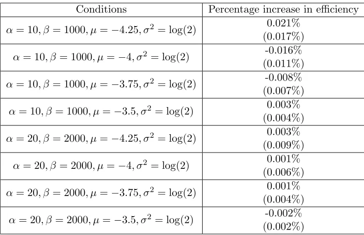
Similarly, since it is unlikely that there will be substantial errors in the estimate of a new ad’s predicted click-through rate, we focus on situations in which there is only moderate uncertainty in the click-through rate of a new ad. In particular, we consider distributions of the CPC bidder’s bid such that the standard deviation in the advertiser’s click-through rate is no greater than 20 or 30% of the expected value. We thus consider values ofα andβ
satisfying (α, β) = (10,1000) and (20,2000) (for 30% and 20% standard errors respectively). Finally, since there is evidence that the distribution of highest bids is well modeled by a lognormal distribution (Lahaie and McAfee, 2011; Ostrovsky and Schwarz, 2009), we assume throughout that the CPM bidder’s bid is drawn from a lognormal distribution with parameters µ and σ2. We use a value of σ2 = log(2) to match the variance in the lognormal distribution estimated by Ostrovsky and Schwarz (2009). And Varian (2009) has noted that the total value enjoyed by advertisers is typically about 2−2.3 times their total expenditure. If the auction consisted of only two advertisers, this would suggest that the appropriate value of µ would be such that the highest competing bidder had a CPM bid that is roughly double that of the CPC bidder in expectation. However, since there are more than two bidders in most real auctions, the appropriate value of µwill be larger than this. We thus consider a range of values ofµfrom −4.25 (for the case in which the highest competing CPM bid is roughly double that of the CPC bidder in expectation) to−3.5 (for the case in which the highest competing CPM bid is roughly four times that of the CPC bidder in expectation).
Conditions Percentage increase in efficiency
α= 10, β= 1000, µ=−4.25, σ2 = log(2) 0.021% (0.017%)
α= 10, β= 1000, µ=−4, σ2 = log(2) -0.016% (0.011%)
α= 10, β= 1000, µ=−3.75, σ2 = log(2) -0.008% (0.007%)
α= 10, β= 1000, µ=−3.5, σ2 = log(2) 0.003% (0.004%)
α= 20, β= 2000, µ=−4.25, σ2 = log(2) 0.003% (0.009%)
α= 20, β= 2000, µ=−4, σ2 = log(2) 0.001% (0.006%)
α= 20, β= 2000, µ=−3.75, σ2 = log(2) 0.001% (0.004%)
α= 20, β= 2000, µ=−3.5, σ2 = log(2) -0.002% (0.002%)
Table 1: Average percentage increase in efficiency from incorporating active learning (with standard errors in parentheses) after 2500 simulations. None of these results are statistically significant at the p < .05 level.
that could be achieved in these settings is at most a few hundredths of a percentage point. These empirical results provide further support for our theoretical conclusions that the value of adding active exploration in an auction setting is exceedingly small.
The reason for the results observed in Table 1 is that an optimal exploration algorithm will only do a tiny additional amount of exploration compared to the greedy strategy of always submitting a bid for the CPC bidder equal to the CPC bidder’s estimated eCPM. For instance, for the first simulation considered in Table 1, the incremental increase in an advertiser’s bid in the first period of the game as a result of active exploration is only 4.2%, implying only a 1.8% increase in the probability that the CPC bidder will be shown as well as only a 2.1% increase in expected payoff conditional on the auctioneer showing a different ad under active exploration than under the purely greedy strategy. Thus the incremental expected payoff increase that can be achieved by incorporating active exploration in this auction setting is at most a few hundredths of a percentage point.
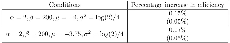
we have assumed in the simulations in Table 1 and we also assume that there is substantially less variance in the distribution of competing CPM bids than we have allowed for in Table 1, then there will be considerably greater benefits to adding active exploration because there is both more to learn about the CPC bidder’s true eCPM bid as well as less exploration that will take place for free solely due to random variation in the competing bids. In this case, there may well be significant benefits to adding active exploration.
Conditions Percentage increase in efficiency
α= 2, β= 200, µ=−4, σ2= log(2)/4 0.15% (0.05%)
α= 2, β= 200, µ=−3.75, σ2 = log(2)/4 0.17% (0.05%)
Table 2: Average percentage increase in efficiency from incorporating active learning (with standard errors in parentheses) after 10000 simulations. These results are both statistically significant at the p < .005 level.
Table 2 reports the results of simulations that were conducted using distributions in which there is substantially more uncertainty about the CPC bidder’s click-through rate and substantially less variance in the CPM bidder’s competing CPM bid than in the distributions considered in Table 1. These simulations indeed reveal statistically significant efficiency gains as a result of active exploration. Nonetheless it is worth noting that the efficiency gains reported in Table 2 are still fairly small. Even when we make assumptions that bias the case in favor of active exploration being important, none of the efficiency gains reported in Table 2 are greater than a few tenths of a percentage point.
Finally, while the gains achieved through active exploration in Table 2 are small, one would not achieve greater gains by using a standard algorithm such as UCB. To test this, we considered the same setting in the first row of this table, but instead of making a bid for the CPC bidder of the formxt+δ(1−δ
T−t)
2(1−δ)
αtβt
(αt+βt)2(αt+βt+1)2f(xt) in each periodt, we made a
bid of the formxt+c(xt)√α1
t+βt, where the constantc(xt) was chosen so that this bid would
equalxt+δ(1−δ
T−t)
2(1−δ)
αtβt
(αt+βt)2(αt+βt+1)2f(xt) in time period t= 1. Thus our implementation
of UCB performed the same amount of exploration as the main algorithm we considered in the very first period of the game, while performing more exploration in later periods due to the fact that the rate of exploration declines with (α 1
t+βt)2 under our proposed algorithm,
while only declining with √ 1
αt+βt under UCB.
12. Conclusion
In online auctions, there may be value to exploring ads with uncertain eCPMs to learn about the true eCPM of the ad and be able to make better ranking decisions in the future. But the online auction setting is very different from standard multi-armed bandit problems because there may be considerable variation in the quality of competition that an advertiser with unknown eCPM faces in an auction, and as a result there will typically be plenty of free opportunities to explore an ad with uncertain eCPM in auctions where there simply are no ads with eCPM bids that are known to be high.
We have presented a model of the explore/exploit problem in online auctions that ex-plicitly considers this random variation in competing bids that is present in real auctions. We find that the optimal solution for ranking the ads is dramatically different than the optimal solution in standard multi-armed bandit problems, and in particular, that the op-timal amount of active exploration is considerably smaller than in standard multi-armed bandit problems. This in turn implies that the improvement in the auctioneer’s payoff that can be achieved by adding active learning in online auctions is also exceedingly small. Thus while it is theoretically possible to improve efficiency by incorporating active learning, in a practical exchange environment, a purely greedy strategy of simply ranking the ads by their expected eCPMs is likely to perform nearly as well as any other strategy.
We conclude by discussing one other point. Throughout our analysis we have focused on the problem of an auctioneer who wants to maximize efficiency. Although this is a sensi-ble objective, one might also envision scenarios in which the mechanism designer wishes to maximize a weighted average of efficiency and revenue. While incorporating active explo-ration in online auctions can only have a small effect on efficiency, this active exploexplo-ration may significantly improve revenue. The reason for this is that if we rank the ads by the sum of their expected eCPMs and a value of learning term, the value of learning term may be larger for ads that typically lose the auctions, and incorporating this value of learning term may increase pricing pressure for the winning ads and thereby increase revenue.8 In fact, in several of the simulations considered in the previous section in which incorporating ac-tive exploration failed to show significant efficiency gains, the algorithm that we considered still showed significant revenue gains over the purely greedy strategy of ranking the ads by their expected eCPMs. But while it is still possible to achieve significant revenue gains by incorporating active exploration in the type of environment considered in this paper, the maximum possible efficiency gains are likely to be exceedingly small.
Acknowledgments
We especially thank Martin Zinkevich for numerous helpful discussions. We are also grateful to Joshua Dillon, Pierre Grinspan, Chris Harris, Tim Lipus, Mohammad Mahdian, Hal Varian, and the anonymous referees for helpful comments and discussions.
This work is based on an earlier work: “Machine Learning in an Auction Environment”, inProceedings of the23rdInternational Conference on the World Wide Web(WWW) (2014)
c
ACM, 2014. http://doi.acm.org/10.1145/2566486.2567974.
Appendix A. Proofs of Theorems
Proof of Theorem 1: Suppose it is known that the eCPM of the ad is x. If the highest eCPM for a competing ad is p, then the presence of this ad with eCPM x increases total welfare by x−p if x > p and 0 otherwise. Thus the expected increase in total welfare from this ad with eCPM of x competing in the auction is Rx
0(x−p)f(p) dp. The total long-term value from having this advertisement is then the discounted sum of this expected total increase in welfare or 1−1δRx
0(x−p)f(p)dp. Now ifV(x)≡ 1−1δRx
0(x−p)f(p)dp, thenV
0(x) = 1 1−δ
Rx
0 f(p)dpandV
00(x) = 1 1−δf(x). From this it follows thatV00(x)≥0 for all xandV00(x)>0 ifx is contained in the support of F. Thus the long-term value of the advertisement is a convex function of the eCPM of the ad and a strictly convex function if the eCPM of the ad is contained within the support of the distribution of the highest competing eCPM.
Proof of Lemma 2: Suppose an ad has been shown k times. The value of the dynamic program that arises from placing the optimal bidzin the current period, Vk(x), equals the immediate reward from biddingz(or the negative of the loss function) in the current period plus δ times the expected value of the dynamic program that arises in the next period.
Now if the new advertiser places a bid of z, then the probability the advertiser wins the auction is F(z), in which case the expected value of the dynamic program that arises next period isEx0[Vk+1(x0)], where the expectation is taken over the randomness in the changes
in the estimates of the eCPM of the ad x0 that arise as a result of showing this ad. The probability the advertiser does not win the auction is 1−F(z), in which case the value of the dynamic program remains at Vk(x). Thus the expected value of the dynamic program that arises in the next period is F(z)Ex0[Vk+1(x0)] + (1−F(z))Vk(x).
At the same time, we have already seen that the reward from bidding z that arises in the current period equals−Rz
x+σkF(z)−F(y)dy. By combining this with the insights in
the previous paragraphs, it follows that
Vk(x) = max z E
−
Z z
x+σk
F(z)−F(y)dy+δ(F(z)Ex0[Vk+1(x0)] + (1−F(z))Vk(x))
.
By subtracting δVk(x) from both sides and dividing by 1−δ, it follows that
Vk(x) = 1 1−δ
max
z E
−
Z z
x+σk
F(z)−F(y)dy+δF(z)(Ex0[Vk+1(x0)]−Vk(x))
.
Proof of Theorem 3: By differentiating the expression in Lemma 2 with respect toz, we see that the first order condition for zto be an optimal bid is
0 = E
−
Z z
x+σk
f(z)dy+δf(z)(Ex0[Vk+1(x0)]−Vk(x))
= E
−f(z)(z−x−σk) +δf(z)(Ex0[Vk+1(x0)]−Vk(x))
= f(z)(x−z+δ(Ex0[Vk+1(x0)]−Vk(x)))
From this it follows that z =x+δ(Ex0[Vk+1(x0)]−Vk(x)) satisfies the first order