A General Framework for Consistency of Principal Component Analysis

A General Framework for Consistency of Principal

Component Analysis

Dan Shen [email protected]

Interdisciplinary Data Sciences Consortium Department of Mathematics and Statistics University of South Florida

Tampa, FL 33620-5700, USA

Haipeng Shen [email protected]

School of Business University of Hong Kong Pokfulam, Hong Kong

J. S. Marron [email protected]

Department of Statistics and Operations Research University of North Carolina at Chapel Hill Chapel Hill, NC 27599-3260, USA

Editor:massimiliano pontil

Abstract

A general asymptotic framework is developed for studying consistency properties of princi-pal component analysis (PCA). Our framework includes several previously studied domains of asymptotics as special cases and allows one to investigate interesting connections and transitions among the various domains. More importantly, it enables us to investigate asymptotic scenarios that have not been considered before, and gain new insights into the consistency, subspace consistency and strong inconsistency regions of PCA and the bound-aries among them. We also establish the corresponding convergence rate within each region. Under general spike covariance models, the dimension (or number of variables) discourages the consistency of PCA, while the sample size and spike information (the relative size of the population eigenvalues) encourage PCA consistency. Our framework nicely illustrates the relationship among these three types of information in terms of dimension, sample size and spike size, and rigorously characterizes how their relationships affect PCA consistency. Keywords: High dimension low sample size, PCA, Random matrix, Spike model

1. Introduction

Principal Component Analysis (PCA) is an important visualization and dimension reduction tool which finds orthogonal directions reflecting maximal variation in the data. This allows the low dimensional representation of data, by projecting data onto these directions. PCA is usually obtained by an eigen decomposition of the sample variance-covariance matrix of the data. Properties of the sample eigenvalues and eigenvectors have been analyzed under several domains of asymptotics.

tradi-tional asymptotic setups as special cases, and furthermore it allows a careful study of the connections among the various setups. More importantly, we investigate a wide range of interesting scenarios that have not been considered before, and offer new insights into the consistency (in the sense that the angle between estimated and population eigen directions tends to 0, or the inner product tends to 1) andstrong-inconsistency (where the angle tends toπ/2, i.e., the inner product tends to 0) properties of PCA, along with some technically challenging convergence rates.

Existing asymptotic studies of PCA roughly fall into four domains:

(a) the classical domain of asymptotics, under which the sample size n → ∞ and the dimension d is fixed (hence the ratio n/d → ∞). For example, see Girshick (1939); Lawley (1956); Anderson (1963, 1984); Jackson (1991).

(b) therandom matrixtheory domain, where both the sample sizenand the dimension

dincrease to infinity, with the ration/d→c, a constant mostly assumed to be within (0,∞). Representative work includes Biehl and Mietzner (1994); Watkin and Nadal (1994); Reimann et al. (1996); Hoyle and Rattray (2003) from the statistical physics literature, as well as Johnstone (2001); Baik et al. (2005); Baik and Silverstein (2006); Onatski (2012); Paul (2007); Nadler (2008); Johnstone and Lu (2009); Lee et al. (2010); Benaych-Georges and Nadakuditi (2011) from the statistics literature.

(c) the high dimension low sample size (HDLSS) domain of asymptotics, which is based on the limit, as the dimension d → ∞, with the sample size n being fixed (hence the ration/d→0). HDLSS asymptotics was originally studied by Casella and Hwang (1982), and rediscovered by Hall et al. (2005). PCA has been studied using the HDLSS asymptotics by Ahn et al. (2007); Jung and Marron (2009).

(d) theincreasing signal strengthdomain of asymptotics, wheren,dare fixed and the signal strength tends to infinity. Such a setting is studied in Nadler (2008).

PCA consistency and (strong) inconsistency, defined in terms of angles, are important properties that have been studied before. A common technical device is the spike covariance model, initially introduced by Johnstone (2001). This model has been used in this context by, for example, Nadler (2008); Johnstone and Lu (2009); Jung and Marron (2009). Re-cently, Ma (2013) formulates sparse PCA (Zou et al., 2006) through iterative thresholding and studies its asymptotic properties under the spike model. An interesting, more general, model has been considered by Benaych-Georges and Nadakuditi (2011).

Under the spike model, the first few eigenvalues are much larger than the others. Amajor message of the present paperis that there are three critical features whose relationships drive the consistency properties of PCA, namely

(1) thesample size: the sample sizenencouragesthe consistency of the sample eigenvec-tors, meaning that more samples tend towards more frequent consistency;

(2) thedimension: the dimensionddiscouragesthe consistency of the sample eigenvectors, meaning that higherdtends towards less frequent consistency;

Our general framework considers increasing sample size n, increasing dimensiond, and increasing spike signal. We clearly characterize how their relationships determine the regions of consistency and strong-inconsistency of PCA, along with the boundary in-between.

Note that the classical domain ((a) above) assumes increasing sample sizenwhile fixing dimensiond; the random matrix domain ((b) above) assumes increasing sample sizen and increasing dimensiond, while fixing the spike signal; the HDLSS domain ((c) above) fixes the sample size, and increases the dimension and the spike signal; the increasing signal strength domain ((d) above) assumes increasing the spike signal, while fixing the sample size and the dimension; thus each of these three domains is a boundary case of our framework. Our theorems, when restricted to these existing domains of asymptotics, are consistent with known results.

In addition, our theorems go beyond these known results to demonstrate the transi-tions among the existing domains of asymptotics, and for the first time to the best of our knowledge, enable one to understand interesting connections among them. Finally, we also establish novel results on rates of convergence.

Sections 3 and 4 formally state very general theorems for multiple component spike models. For illustration purposes only, in this section we first consider Examples 1 and 2 under some strong assumptions, which provide intuitive insights regarding the much more general theory presented in Sections 3 and 4. In addition, we use Example 3 to show the application of our theoretical study to the factor model considered by Fan et al. (2013).

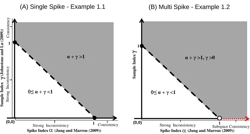
For Examples 1 and 2, to better demonstrate the connection with existing results, the three types of features (sample size, dimension, and spike signal) and their relationships are mathematically quantified by two indices, namely the spike index α and the sample index γ. Within the context of these examples, we point out the significant contributions of our results in comparison with existing results. The comparisons and connections are graphically illustrated in Figure 1 and discussed below.

Example 1 Single-component Spike Model Assume that X1, . . . , Xn are sample vec-tors from a d-dimensional distribution with zero mean and covariance matrix Σ, where the entries ofΣ−12X_i are i.i.d. random variables with zero mean, unit variance and finite fourth moment. (A special case: Xi is from the d-dimensional normal distribution N(0,Σ)). In addition, assume that the sample size n=dγ (γ ≥0 is defined as the sample index), and the covariance matrix Σ has the following eigenvalues:

λ1=c1dα, λ2 =· · ·=λd= 1, α≥0, where the constant α is defined as the spike index.

Corollary B.2in the supplementary materials, when applied to this example, shows that the maximal sample eigenvector is consistent when α+γ >1(grey region in Figure 1(A)), and strongly inconsistent when 0≤α+γ <1 (white triangle in Figure 1(A)). These very general new results nicely connect with many existing ones:

• Previous Results I - the classical domain:

(A) Single Spike - Example 1.1 (B) Multi Spike - Example 1.2

γ

S

am

p

le Ind

ex

(

Joh

n

stone

an

d

L

u

(2009

))

0≤ α + γ <1

1

1 Spike Index (Jung and Marron (2009)) a

α + γ >1

Consistency

Strong Inconsistency

C

onsi

stenc

y

S

trong

I

nc

onsi

stenc

y

(0,0)

S

am

p

le Ind

ex

Spike Index (Jung and Marron (2009)) a

0≤ α + γ <1

1

1

α + γ >1, γ >0

Subspace Consistency Strong Inconsistency

(0,0)

γ

Figure 1: General consistency and strong inconsistency regions for PCA, as a function of the spike index α and the sample index γ. Panel (A) - single spike model in Example 1: PCA is consistent in the grey region (α +γ > 1), and strongly inconsistent on the white triangle (0 ≤ α+γ < 1). Panel (B) - multiple spike model in Example 2: the first m sample PCs are consistent in the grey region (α+γ >1, γ > 0), subspace consistent on the dotted line (α >1, γ = 0) on the horizontal axis, and strongly inconsistent on the white triangle (0≤α+γ <1).

• Previous Results II - the random matrix domain:

(a) Assuming normality, the results of Johnstone and Lu (2009) appear on the ver-tical axis in Panel (A) where the spike index α= 0 (as they fix the spike infor-mation): the first sample eigenvector is consistent when the sample index γ >1 and strongly inconsistent when γ <1.

(b) Again, under the normal assumption, Nadler (2008) explored the interesting boundary case of α = 0, γ = 1 (i.e. d_n → c for a constant c) and showed that

<uˆ1, u1 >2 a .s

−→ ((λ1−1)2−c)+

(λ1−1)2+c(λ1−1), whereuˆ1 andu1 are the first sample and popula-tion eigenvector. This result appears in Panel (A) as the single solid circleγ = 1 on the vertical axis. Our general framework doesn’t cover this boundary case and this boundary result is a complement of our theoretical results.

• Previous Results III - the HDLSS domain:

(b) Under the normal assumption, Jung et al. (2012) deeply explored limiting behav-ior at the boundary α= 1, γ= 0 (i.e. _λd

1 →c for a constant c) and showed that

<uˆ1, u1 >2⇒ _AA_+c, where “⇒” means convergence in distribution and A∼χ2n, the chi-squared distribution with n degrees of freedom. This result appears in Panel (A) as the single solid circle α= 1 on the horizontal axis. This boundary case is again a complement of our general framework.

• Our Resultshence nicely connect existing domains of asymptotics, and give a much more complete characterization for the regions of PCA consistency, subspace consis-tency, and strong inconsistency. We also investigate asymptotic properties of the other sample eigenvectors and all the sample eigenvalues.

Example 2 Multiple-component Spike Model Assume that the covariance matrix Σ in Example 1 has the following eigenvalues:

λj = (

cjdα if j≤m,

1 if j > m, α≥0,

where m is a finite positive integer, the constants cj, j = 1,· · · , m, are positive and satisfy thatcj > cj+1>1, j= 1,· · ·, m−1.

Corollary B.1in the supplementary materials, when applied to this example, shows that the first m sample eigenvectors are individually consistent with corresponding population eigenvectors when α+γ > 1, γ > 0 (the grey region in Figure 1(B)), instead of being subspace consistent (Jung and Marron, 2009), and strongly inconsistent when α+γ < 1 (the white triangle in Panel (B)). This very general new result connects with many others in the existing literature:

• Previous Results I - the classical domain:

Assuming normality, Theorem 1 of Anderson (1963) implied that for fixed dimension

d and finite eigenvalues, when the sample sizen→ ∞ (i.e. γ → ∞, the limit on the vertical axis), the first m sample eigenvectors are consistent, while the other sample eigenvectors are subspace consistent. This case is the upper left corner of Figure 1(B).

• Previous Results II - the random matrix domain:

The following results are under the normal assumption. Paul (2007) explored asymp-totic properties of the firstmeigenvectors and eigenvalues in the interesting boundary case of α = 0, γ = 1, i.e., _nd → c with c ∈ (0,1) and showed that < uˆj, uj >2 a

.s

−→

((λj−1)2−c)+

(λj−1)2+c(λj−1) for j = 1,· · · , m. This result appears in Panel (B) as the solid

• Previous Results III - the HDLSS domain:

The theorems of Jung and Marron (2009) are valid on the horizontal axis in Panel (B) where the sample indexγ = 0. In particular, for this example, their results showed that the first m sample eigenvectors are not respectively consistent with the corresponding population eigenvectors when the spike index α > 1 (the horizontal dotted red line segment), instead they are subspace consistent with their corresponding population eigenvectors, and are strongly inconsistent when the spike indexα <1 (the horizontal solid line segment). They and Jung et al. (2012) did not study the asymptotic behavior on the boundary - the single open circle (α= 1, γ= 0) on the horizontal axis.

• Our Results cover the classical domain, and are stronger than what Jung and Mar-ron (2009) obtained: the increasing sample size enables us to separate out the first few leading eigenvectors and characterize individual consistency, while only subspace consistency was obtained by Jung and Marron (2009).

Example 3 The Factor Model of Fan et al. (2013)Consider the following model:

yt=Bft+Et,

where yt = (yt,1, . . . , yt,d)T is the d-dimensional response vector, B = (b1, . . . ,bd)T is the d×m (m is fixed) loading matrix, ft is the m×1 vector of common factors, and Et= (et,1, . . . , et,d)T is thed-dimensional noise vector, t= 1, . . . ,T. The noise vector Et is independent of ft. Then the population covariance matrix of yt is

Σ =Bcov(ft)BT + ΣE,

where ΣE is the covariance matrix ofEt. Fan et al. (2013) assumes that the first m eigen-values of Bcov(ft)BT increase with d as d → ∞, whereas all the eigenvalues of ΣE are bounded. It then follows that λm(Σ)λm+1(Σ) · · · λd(Σ)1, as d→ ∞. Then our theorems are applicable to this factor model whenf1, . . . ,f_T is i.i.d., andE1, . . . ,E_T is i.i.d.. Under the above assumptions of the factor model, we have d/(Tλm(Σ)) → 0. Then according to our Theorem 1 (together with the third comment after the theorem), the firstm

sample eigenvalues and eigenvectors are consistent. On the other hand, Fan et al. (2013) proposed the consistent principal orthogonal complement thresholding (POET) estimator for the covariance matrix Σ, which is obtained by keeping the first m sample eigenvalues and eigenvectors, and thresholding the residual sample matrix. Hence, our theorem offers another theoretical support on the consistency of their POET estimator.

the relevant lemmas. The supplementary materials contain the corresponding corollaries of Theorems 1 and 2, for multiple-spike models with distinct eigenvalues and single spike models, along with the proofs of Theorem 2 and all the corollaries.

2. Notations and Concepts

We now introduce some necessary notations, and define consistency concepts relevant for our asymptotic study.

2.1 Notation

Let the population covariance matrix be Σ, whose eigen decomposition is

Σ =UΛUT,

where Λ is the diagonal matrix of population eigenvaluesλ1 ≥λ2 ≥. . .≥λd, and U is the matrix of the corresponding eigenvectors U = [u1, . . . , ud].

As in Jung and Marron (2009), assume thatX1, . . . , Xnare i.i.d. d-dimensional random sample vectors and have the following representation

Xi =

d X

j=1

λ

1 2

jzi,juj, (1)

where thezi,j’s are i.i.d. random variables with zero mean, unit variance, and finite fourth moment. An important special case is that they follow the standard normal distribution.

Assumption 1 X1, . . . , Xn are a random sample having the distribution of (1). Jung and Marron (2009) assumes that

Zi = (zi,1,· · · , zi,d)T, i= 1,· · ·, n, (2) are independent and the elementszi,j withinZi areρ-mixing. This assumption leads to the convergence in probability results under the HDLSS domain in Jung and Marron (2009). Here we assume that the elementszi,j withinZi are also independent. This helps to get the almost sure convergence results under our general framework, which includes the HDLSS domain. Assumption 1 is necessary to satisfy the conditions of Lemma 1 - the Bai-Yin’s law (Bai and Yin, 1993), which is important for our results, for example, Theorem 1.

Denote the sample covariance matrix by ˆΣ =n−1_XXT_{, whereX = [X}

1, . . . , Xn]. Note that ˆΣ can also be decomposed as

ˆ

Σ = ˆUΛ ˆˆUT, (3)

where ˆΛ is the diagonal matrix of sample eigenvalues ˆλ1 ≥ λˆ2 ≥ . . . ≥ ˆλd, and ˆU is the matrix of corresponding sample eigenvectors where ˆU = [ˆu1, . . . ,uˆd].

• Denoteξτ = oa.s(aτ) if limτ→∞ξ_aτ

τ = 0 almost surely.

• Denoteξτ = Oa.s(aτ) if limτ→∞

ξτ

aτ

≤M, whereM is a positive constant.

• Denote almost surely ξτ aτ ifc2 ≤limτ→∞aξττ ≤limτ→∞

ξτ

aτ ≤c1 almost surely, for

two constantsc1 ≥c2 >0.

In addition, we introduce the following notions to help understand the assumptions on the population eigenvalues in our theorems and corollaries. Assume that{aτ :τ = 1, . . . ,∞} and {bτ :τ = 1, . . . ,∞}are two sequences of real valued numbers.

• Denoteaτ bτ if limτ→∞_abτ

τ = 0.

• Denoteaτ bτ ifc2≤limτ→∞abττ ≤limτ→∞

aτ

bτ ≤c1 for two constants c1≥c2>0.

2.2 Concepts

We now list several concepts about consistency and strong inconsistency, some of which are modified from the related concepts in Jung and Marron (2009) and Shen et al. (2013).

LetH be an index set, e.g. H={m+ 1,· · · , d}, and then denoteS= span{uk, k∈H} as the linear span generated by {uk, k ∈H}. Define angle(ˆuj, S) as the angle between the estimator ˆujand the subspaceS, which is the angle between the estimator and its projection onto the subspace (Jung and Marron, 2009). For further clarification, we provide a graphical illustration of the angle in Section B of the supplement (Shen et al., 2015). As pointed out earlier, letτ stand for eithernord, depending on the context.

• If as τ → ∞, angle(ˆuj, S) a.s

→ 0, then ˆuj is subspace consistent with S. If H only includes one index j such that S = span{uj}, then angle(ˆuj, S)

a.s

→0 is equivalent to

|<uˆj, uj >|→a.s1, and ˆuj isconsistent withuj.

• If asτ → ∞,|<uˆj, uj >|a→.s 0, then ˆuj is strongly inconsistent withuj.

3. Cases with increasing sample size n

We study spike models with increasing sample size n → ∞ in this section. As such, the eigenvalues λj and the dimension d depend on the sample size n, and will be denoted as

λ(_jn) and d(n) throughout this section. They can be viewed as sequences of constant values indexed by n. This section considers multiple-component spike models with inseparable eigenvalues and presents the main theorem of our paper. Section B of the supplemen-tary materials reports the corollaries for multiple component spike models with distinct eigenvalues and single spike models.

We consider multiple spike models with m (a finite integer) dominating eigenvalues. These m eigenvalues can be grouped into r tiers, where the eigenvalues within the same tier have the same limit. To fixed ideas, the first m eigenvalues are grouped into r tiers where there are ql(> 0) eigenvalues in the lth tier with

Pr

qr+1 =d(n)−Prl=1ql, and the index set of the eigenvalues in the lth tier as

Hl =

(_l−1

X

k=0

qk+ 1, l−1 X

k=0

qk+ 2,· · ·, l−1 X

k=0

qk+ql )

, l= 1,· · ·, r+ 1. (4)

Assume the eigenvalues in the lth tier have the same limit δ_l(n)(>0), i.e. Assumption 2 limn→∞

λ(_jn)

δ(_ln) = 1, j∈Hl, l= 1,· · · , r.

According to the above assumption, the eigenvalues that are in the same tier will have the same limit as n goes to infinity. As a result, we can show that the corresponding sample eigenvectors can not be consistently estimated individually. This motives us to con-sider subspace consistency. In addition, we assume that the first m population eigenvalues from different tiers are asymptotically different, and dominate the additional population eigenvalues beyond the firstr tiers that have the same limit cλ:

Assumption 3 as n→ ∞, δ(₁n)>· · ·> δ(rn)> λ(mn+1) → · · · →λ (n)

d(n)→cλ >0. For i < j, δ_i(n)> δ(_jn) means that limn→∞δ

(n)

i

δ_j(n) >1. This assumption allows δ (n)

i → ∞ and

δ_i(n) δ(_jn), which is not the case in Paul (2007). Regarding the constant cλ, the second remark after Theorem 1 discusses what happens when cλ = 0.

The above assumptions cover a general class of multiple spike models with tiered eigen-values. A simple special case is the one where the eigenvalue matrix Λ is block diagonal: for 1≤h≤r, theh-th block of Λ isλ(_hn)Iqh where Iqh is the qh×qh identity matrix, with

λ(₁n)> λ(₂n)> . . . > λ_r(n), q1+q2+. . .+qr=m < d; and the last block of Λ iscλId(n)−m withcλ < λ(rn).

Under the above setup, Theorem 1 shows that the eigenvector estimates are either sub-space consistent with the linear sub-space spanned by the population eigenvectors, or strongly inconsistent. As discussed in the Introduction, Theorem 1 considers the delicate balance among the sample size n, the spike signal δ_l(n), and the dimension d(n), and character-ize the various PCA consistency and strong-inconsistency regions. The three scenarios of Theorem 1 are arranged in the order of a decreasing amount of signal:

• Theorem 1(a): If the amount of signal dominates the amount of noise up to the

rth tier, i.e. d(n) nδ(rn)

→ 0, then the estimates for the eigenvectors in the first r tiers

are subspace consistent, and the estimates for the higher order eigenvectors are also subspace consistent (but) at a different rate;

• Theorem 1(b): Otherwise, if the amount of signal dominates the amount of noise only up to thehth tier (1≤h < r), i.e. d(n)

nδ_h(n) → 0 and d(n)

• Theorem 1(c): Finally, if the amount of noise always dominates, i.e. d(n)

nλ(₁n) → ∞, then the sample eigenvalues are asymptotically indistinguishable, and the sample eigenvec-tors are strongly inconsistent.

Before stating Theorem 1, we first introduce several notations. Define the subspace

Sl= span{uk, k∈Hl} forl= 1,· · · , r+ 1 and denoteδ0(n)=∞ for everyn.

Theorem 1 Under Assumptions 1, 2 and 3, as n→ ∞, the following results hold.

(a) If d(n) nδr(n)

→0, then λˆj

λ(_jn) a.s

→1,j = 1,· · · , m, and angle(ˆuj, Sl) = oa.s

δ(_ln) δ_l(−n)1

∨δ

(n)

l+1 δ(_ln)

1₂!

,

j∈Hl, l= 1,· · · , r−1. In addition,

• If d(_nn) → 0, then angle(ˆuj, Sl) = oa.s

δ(_ln) δ_l(₋n)₁ ∨

1 δ(_ln)

1₂!

, j ∈ Hl for l =r, and

oa.s

n 1 δ(rn)

o1₂

for l=r+ 1.

• If d(_nn) →c,0< c≤ ∞, then angle(ˆuj, Sl) = oa.s

δ(_ln) δ(_l−n)₁

1₂!

∨Oa.s

d(n) nδ_l(n)

1₂!

,

j∈Hl for l=r, andOa.s

n d(n) nδ(rn)

o1₂

for l=r+ 1.

(b) If d(n)

nδ(_hn) → 0 and d(n)

nδ(_hn₊₁) → ∞, where 1≤h < r, then ˆ λj

λ(_jn) a.s

→ 1, j ∈ Hl, l = 1,· · ·, h,

and the other non-zero nˆλj

d(n) a.s

→cλ. In addition, angle(ˆuj, Sl) = oa.s

δ(_ln) δ_l(₋n)₁ ∨

δ(_l+1n) δ(_ln)

1₂!

,

j∈Hlforl= 1,· · · , h−1, andoa.s

δ(_hn) δ_h(n₋)₁

1₂!

∨Oa.s

d(n) nδ(_hn)

1₂!

forl=h. Finally,

| < uˆj, uj > | = Oa.s

nλ(_jn) d(n)

1₂!

, j ∈ Hl, l = h+ 1,· · · , r, and Oa.s

n n d(n)

o1₂

,

j > m.

(c) If d(n)

nδ(₁n) → ∞, then the non-zero nλˆj

d(n) a.s

→cλ. In addition,|<uˆj, uj >|= Oa.s

nλ(_jn) d(n)

1₂!

,

j= 1,· · ·, m, and Oa.s

n n d(n)

o1₂

, j > m.

The following comments can be made for the results of Theorem 1.

• Note that, for j ∈H1, the subspace consistency rate for ˆuj is

δ₂(n) δ₁(n)

1₂

. By defining

δ₀(n) =∞, the consistency rate expression

δ(_ln) δ(_l−n)1

∨δ

(n)

l+1 δ_l(n)

1₂

• Ifcλ = 0 in Assumption 3, then that assumption can be rewritten as

δ∗(₁n)>· · ·> δ∗(_rn)> λ∗_m(n₊₁) → · · · →λ∗(_dn_(n)₎ = 1,

whereδ∗(_jn) = δ (n)

j

λ(_dn_(n)₎ andλ

∗(n)

j =

λ(_jn)

λ(_dn_(n)₎. We comment that the asymptotic properties of

ˆ

uj then depend on the rescaled eigenvaluesλ∗(_jn), instead of the raw eigenvalues λ(_jn). In particular, withcλ = 0, Theorem 1 can be slightly modified by replacing δj(n) with

δ∗(_jn), “nˆλj

d(n) a.s

→cλ” with “ n ˆ λj

d(n)λ(_dn_(n)₎ a.s

→1”, and the strongly inconsistency rate

nλ(_jn) d(n)

1₂

with

nλ∗(n)

j

d(n)

1₂

, respectively.

• In Assumption 3, if there is a big gap betweenδr(n) andλ(_mn₊₁) such thatδr(n)λ(_mn₊₁) , thenλ(_mn₊₁) → · · · →λ(_dn_(n)₎→cλ can be weakened toλ(mn+1) · · · λ

(n)

d(n)1. It follows that the consistency results of the first r tiers of sample eigenvalues in Scenario (a) or the firsthtiers in Scenario (b) remain the same, while all other results of the form “ −→a.s ” for the sample eigenvalues should be replaced by almost surely “ ”. The results for the sample eigenvectors remain the same.

• One needs λ(_mn₊₁) → · · · → λ_d(n_(n)₎ → cλ, or λ(mn+1) · · ·λ (n)

d(n) 1, to obtain general convergence results for the non-spike sample eigenvalues ˆλj, j > m, under the wide range of scenarios: d(_nn) → 0, d(_nn) → ∞, or limn→∞d(_nn) = c (0 < c < ∞). When

one focusses only on the spike eigenvalues, a weaker assumption, such as the slowly decaying non-spike eigenvalues assumed by Bai and Yao (2012), is sufficient. Then, the spike condition δr(n) λ(_mn₊₁) is enough to generate the consistency properties of ˆ

λj and ˆuj, j ≤ m in Scenario (a). In that case, the behaviors of the other sample eigenvalues and eigenvectors are scenario specific, depending on whether d(_nn) → 0,

d(n)

n → ∞, or limn→∞ d(n)

n =c(0< c <∞).

• The cases covered by Theorem 1 are not studied in Paul (2007), where the eigenvalues are considered to be individually estimable.

• In Theorem 1, the dimension dcan be fixed. In addition, suppose ∞> δ₁(n) >· · ·> δr(n) > λ(mn+1) → · · · → λ

(n)

d → cλ, and the eigenvalues satisfy Assumption 2. Then, the results of Theorem 1(a) are consistent with the classical asymptotic subspace consistency results implied by Theorem 1 of Anderson (1963).

4. Cases with fixed n

Theorem 2 summarizes the results for spike models with tiered eigenvalues. In compar-ison with Jung and Marron (2009), we make more general assumptions on the population eigenvalues, and obtain the convergence rate results; furthermore, we obtain almost sure convergence, instead of convergence in probability.

Assume that as d→ ∞, the first m eigenvalues fall into r tiers, where the eigenvalues in the same tier are asymptotically equivalent, as stated in the following assumption:

Assumption 4 for fixed n, asd→ ∞, λ(_jd)δ_l(d), j∈Hl, l= 1,· · · , r.

Different from Assumption 2 for diverging sample size n, now with a fixedn, the eigen-values within the same tier are assumed to be of the same order, rather than of the same limit when nincreases to ∞. As we will see below in Theorem 2, one can no longer sepa-rately estimate the eigenvalues of the same order whenn is fixed, which is feasible with an increasing nas long as they do not have the same limit as shown in Theorem 1.

In addition, we assume that the population eigenvalues from different tiers are of different orders and dominate the higher-order eigenvalues which are asymptotically equivalent:

Assumption 5 for fixed n, asd→ ∞, δ(₁d) · · · δr(d)λ(md)+1 · · · λ (d) d 1.

Note that for fixednandd→ ∞, the assumptionδ_l(d)> δ_l(₊₁d) can not guarantee asymptotic separation of the corresponding sample eigenvalues ˆλj for j ∈Hl and j ∈Hl+1. Thus, we need to replace Assumption 3 with Assumption 5 in order to asymptotically separate the first r subgroups of sample eigenvalues.

Before formally stating Theorem 2, we first introduce several notations. Denoteδ₀(d)=∞

for everyd, which is used to describe the subspace consistent rates. Consider thezi,j in (1), and let

e

Zj = (z1,j,· · · , zn,j)T, j = 1,· · · , d. (5) Define

K = lim d→∞

Pd

j=m+1λ (d) j

d and A

∗

l = 1

n

X

k∈Hl

e

ZkZe_kT, l= 1,· · ·, r, (6)

which are used to describe the asymptotic properties of the sample eigenvalues.

Theorem 2 Under Assumptions 1, 4 and 5, for fixed n, as d→ ∞, the following results hold.

(a) If d

δ_h(d) → 0 and d

δ_h(d₊₁) → ∞, where 1 ≤h ≤r, then for j ∈ Hl, l = 1,· · ·, h, almost surely

λmin(A∗l)×mink∈Hlλ

(d)

k ≤λˆj ≤λmax(A

∗

l)×maxk∈Hlλ

(d)

k , (7)

and the other non-zeroˆλj satisfy n ˆ λj

d a.s

→K. In addition, angle(ˆuj, Sl) = oa.s

δ(_ld) δ_l(₋d)₁ ∨

δ_l(₊₁d) δ_l(d)

1₂!

,

j∈Hl forl= 1,· · ·, h−1, andoa.s

δ(_hd) δ_h(d₋)₁

1₂!

∨Oa.s

d δ_h(d)

1₂!

forl=h. Finally,

|<uˆj, uj >|= Oa.s

λ(_jd) d

1₂!

, j∈Hl, l=h+ 1,· · ·, r, and Oa.s

₁

d 1 2

(b) If d

δ(₁d) → ∞, then the non-zero nˆλj

d a.s

→K. In addition,|<uˆj, uj >|= Oa.s

λ(_jd) d

1₂!

,

j= 1,· · ·, m, and Oa.s

₁

d 1 2

, j > m.

The following comments can be made about the results of Theorem 2.

• Even if the non-spike eigenvalues λ(_jd), j > m, decay slowly, the condition δ₁(d) · · · δ(rd) λ_m(d₊₁) can still guarantee the same properties for ˆλj and ˆuj, j ∈ Hl,

l≤h, in Scenario (a).

• Assumption 1 assumes that the zi,j’s are i.i.d. rather than ρ-mixing as in Jung and Marron (2009). Thus, convergence in probability in Jung and Marron (2009) is strengthened to almost sure convergence here.

5. Discussions

Throughout the paper, we assume that the small eigenvalues have the same limit or are of the same order as 1, i.e. λ(_mn₊₁) → · · · →λ_d(n_(n)₎ →cλ orλ

(n)

m+1 · · · λ (n)

d(n)1. In fact, this is a convenient choice. Our results remain valid when these small eigenvalues are not of the same order, and even when some of them are 0. For example, supposeλd1+1 =· · ·=λd= 0 for m+ 1 < d1 < d. As shown in Section E of the supplementary material (Shen et al., 2015), the asymptotic properties of PCA are independent of the basis choice for the d -dimensional space. If the population eigenvectors uj, j = 1, . . . , d, are chosen as the basis of the d-dimensional space, the population covariance matrix becomes

Σ = Λ =

Λ1 0d1×(d−d1) 0_(d−d1)×d1 0(d−d1)×(d−d1)

, where Λ1 = 

 

λ1 · · · 0 ..

. . .. ... 0 · · · λd1





,

and 0k×l is thek-by-lzero matrix. Then, the asymptotic properties of PCA under the pop-ulation covariance matrix Σ is the same as those under the covariance matrix Λ1. Therefore, we only need to replace the dimension d by the effective dimension d1, and all the earlier results remain valid.

It would be interesting to explore non-asymptotic results under our general framework. There have been interesting relevant progresses made recently. Koltchinskii and Lounici (2016, 2015) consider a general framework that encompasses the spike model with fixed spike sizes, and establish theorems about non-asymptotic properties of sample eigenval-ues/eigenvectors under either Gaussian or centered subgaussian assumption. These results pave the way to study non-asymptotic properties under our framework where the spike sizes are allowed to grow and we only assume finite fourth moment.

6. Acknowledgements

Health Challenge Grant 1 RC1 DA029425-01. We thank the action actor and the four referees for their helpful comments and suggestions.

7. Proofs

We now provide the detailed proof for Theorem 1. To save space, the proofs for Theorem 2 and the corresponding corollaries of the two theorems (which are often similar, and simpler) are provided in the supplement (Shen et al., 2015). We first provide some overview in Section 7.1 and list four lemmas in Section 7.2, and then derive the asymptotic properties of the sample eigenvalues and the sample eigenvectors in Sections 7.3 and 7.4, respectively. We study the consistency and strong inconsistency of PCA through the angle or the inner product between a sample eigenvector and the corresponding population eigenvec-tor. We first note that this angle has a nice invariance property: it doesn’t depend on the specific choice of the basis for thed-dimensional space, as discussed in details in the supple-ment (Shen et al., 2015). Given this invariance property, for the rest of the paper, we choose to use the population eigenvectors uj, j = 1, . . . , d(n), as the basis of the d-dimensional space, which is equivalent to assuming that Xi, i = 1, . . . , n, is a d-dimensional random vector with mean zero and a diagonal covariance matrix as Σ = Λ = diag{λ(₁n), . . . , λ_d(n_(n)₎}. This will simplify our mathematical analysis, see for example (32) and (33).

Define jl to be the largest index in Hl and then jl =Plk=0qk,l = 1,· · · , r. Note that

jr=Pr_k=0qk=m. Since the firstm eigenvalues are grouped into r tiers in Assumption 2, then Assumption 2 can be rewritten as

λ(₁n) δ₁(n)

→ · · · → λ

(n) j1

δ(₁n)

→1, · · · , λ

(n) jr−1+1

δ(rn)

→ · · · → λ

(n) jr

δr(n)

→1. (8)

7.1 Overview

Our proof makes use of the connection between the sample covariance matrix ˆΣ and its dual matrix ˆΣD, which share the same nonzero eigenvalues. Since Σ = Λ = diag{λ(1n), . . . , λ

(n) d(n)}, then it follows from (1) and (5) that the dual matrix can be expressed as

ˆ

ΣD =n−1XTX = 1

n

d(n) X

j=1

λ(_jn)Ze_jZe_jT,

where Ze_j is the n-dimensional random vector and its elements are i.i.d random variables with zero mean, unit variance, and finite fourth moment. Furthermore, the dual matrix can be rewritten as the sum of two matrices as follows:

ˆ

ΣD =A+B, with A= 1

n

m X

j=1

λ(_jn)Ze_jZe_jT, B= 1

n

d(n) X

j=m+1

λ(_jn)Ze_jZe_jT. (9)

the dual matrix ˆΣD in Section 7.3. Finally, we derive the asymptotic properties of the sample eigenvectors of ˆΣ in Section 7.4. Some intuitive ideas are provided in the supplement (Shen et al., 2015) to help understanding the proof.

7.2 Lemmas

We list four lemmas that are used in our proof. Lemma 1 studies asymptotic properties of the largest and smallest non-zero eigenvalues of a random matrix.

Lemma 1 Suppose B = 1_qV VT where V is an p×q random matrix composed of i.i.d. random variables with zero mean, unit variance and finite fourth moment. As q→ ∞ and

p

q → c∈[0,∞), the largest and smallest non-zero eigenvalues of B converge almost surely to (1 +√c)2 and (1−√c)2, respectively.

Remark 1 Lemma 1 is known as the Bai-Yin’s law (Bai and Yin, 1993). As in Remark 1 of Bai and Yin (1993), the smallest non-zero eigenvalue is thep−q+ 1 smallest eigenvalue of B for c >1.

Lemma 2 is about the Weyl Inequality and the dual Weyl Inequality (Tao, 2010), which appear below as the right-hand-side inequality and the left-hand-side inequality, respec-tively.

Lemma 2 If A, B are p×p real symmetric matrices, then for all j= 1, . . . , p,

    

   

λj(A) + λp(B)

λj+1(A) + λp−1(B) ..

.

λp(A) + λj(B)     

   

≤λj(A+B)≤     

   

λj(A) + λ1(B)

λj−1(A) + λ2(B) ..

.

λ1(A) + λj(B)     

   

,

where λj(·) is the j-th largest eigenvalue of the matrix.

Lemma 3 As n→ ∞, the eigenvalues of the matrixA in (9) satisfy

λj(A)

λ(_jn)

a.s

−→1, for j= 1,· · · , m.

Proof Define the m-dimensional random vectors X_i∗ = Im,0m×(d−m)

Xi, i = 1,· · ·, n. Then,X_i∗ has mean zero and the following covariance matrix Σ∗:

Σ∗= 

 

λ(₁n) · · · 0 ..

. . .. ... 0 · · · λ(mn)





LetA∗ be the dual matrix of the matrixA. The sample covariance matrix ofX_i∗ is

A∗ = 1

n

n X

i=1

X_i∗X_i∗T

= λ(₁n)×

        1 n Pn

i=1z2i,1 · · ·

λ(mn)

λ(₁n)

1₂

1 n

Pn

i=1zi,1zi,m ..

. . .. ...

λ(mn)

λ(₁n)

1₂

1 n

Pn

i=1zi,1zi,m · · · λ (n)

m

λ(₁n) 1 n

Pn

i=1zi,m2         , (10)

where thezi,j’s are defined in (1).

Since A∗ is the dual matrix ofA, then A and A∗ share the same non-zero eigenvalues. Below we study the eigenvalues ofA through the dual matrixA∗.

The i.i.d. and unit variance properties of thezi,j’s yield that as n→ ∞,

1

n

n X

i=1

zi,kzi,l a.s

−→

1 1≤k=l≤m

0 1≤k6=l≤m . (11)

Denote bk = limn→∞λ

(n)

k

λ(₁n) ≤ 1, k = 1,· · ·, m. Then it follows from (10) and (11) that as

n→ ∞,

1

λ(₁n)

A∗ −→a.s



 

1 · · · 0 ..

. . .. ... 0 · · · bm





,

which further yields

λ1(A)

λ(₁n)

= λ1(A

∗₎

λ(₁n)

a.s

−→1. (12)

Similarly, for k= 2,· · · , m, we have that as n→ ∞,

λ1(_n1Pmj=kλ (n) j Ze_jZe_jT)

λ(_kn)

a.s

−→1. (13)

Next we derive the upper and lower bounds for λk(A), k = 2,· · ·, m. According to Lemma 2, we have the following inequality :

λk(A) =λk( 1

n

m X

j=1

λ(_jn)Ze_jZe_jT)≤λ1( 1

n

m X

j=k

λ(_jn)Ze_jZe_jT) +λ_k( 1

n

k−1 X

j=1

λ(_jn)Ze_jZe_jT).

Since the rank of 1_nPk−1 j=1λ

(n)

j Ze_jZe_jT is at mostk−1, thenλ_k(1_n

Pk−1

j=1λ (n)

j Ze_jZe_jT) = 0, which together with (13), yields that

λk(A)

λ(_kn)

≤ 1

λ(_kn)

×λ1( 1

n

m X

j=k

For the lower bound, it follows from Equation (5.9) in Jung and Marron (2009) that

λ1(λ (n) k

n ZekZe

T

k) +λn( 1

n

m X

j=k+1

λ_j(n)Ze_jZe_jT)≤λ_k(A). (15)

Given that the rank of_n1Pm j=k+1λ

(n)

j Ze_jZe_jT is at mostmwithm < n, thenλ_n(_n1

Pm

j=k+1λ (n)

j Ze_jZe_jT) = 0, which together with (15), yields that

λk(A)

λ(_kn)

≥ 1

λ(_kn)

×λ1(

λ(_kn) n ZekZe

T

k). (16)

Note that asn→ ∞,

1

λ(_kn)

×λ1(λ (n) k

n ZekZe

T k) =

1

nZe

T kZe_k

a.s

−→1. (17)

It follows from (13), (14), (16) and (17) that, for k= 2,· · · , m,

λk(A)

λ(_kn)

a.s

−→1, as n→ ∞. (18)

The combination of (12) and (18) proves Lemma 6.1.

Lemma 4 Assume that limn→∞d(_nn) = c, where 0 ≤ c ≤ ∞, and let λmax(·) and λmin(·) be the largest and smallest non-zero eigenvalues of the matrix, respectively. As n → ∞,

λmax(B) and λmin(B), where B in (9), satisfy

λmax(B) and λmin(B) →a.scλ, for c= 0, (19)

n

d(n)λmax(B) and

n

d(n)λmin(B) a.s

→cλ, for c=∞, (20)

and

λmax(B)→a.s cλ(1 +

√

c)2 and λmin(B)a→.scλ(1−

√

c)2, for 0< c <∞. (21)

Remark 2 If λ(_mn₊₁) → · · · →λ_d(n_(n)₎ is relaxed toλ_m(n₊₁) · · · λ(_dn_(n)₎, then “a→.s ”is replaced by almost surely “”.

Proof Define B∗ = _n1Pd(n)

j=m+1Ze_jZe_jT. The proof uses the following inequalities fork≥1:

We first prove the right inequality of (22). Note that λ(_mn₊₁) B∗ can be rewritten as

λ(_mn₊₁) B∗ =B+B_R∗, whereB_R∗ = _n1Pd(n) j=m+1(λ

(n)

m −λ(jn))Ze_jZe_jT and is a non-negative matrix. It then follows from Lemma 2 that for k≥1,

λ(_mn₊₁) ×λk(B∗) =λk(λ(_mn₊₁) B∗)≥λk(B) +λn(BR∗)≥λk(B), which yields the right inequality of (22).

For the left inequality in (22), note thatB=λ(_dn_(n)₎B∗+B∗_L, whereB∗_L= 1_nPd(n) j=m+1(λ

(n) j −

λ(_dn_(n)₎)Ze_jZe_jT and is a non-negative matrix. Lemma 2 implies that for k≥1,

λk(B)≥λk(λ_d(n_(n)₎B∗) +λn(B∗L)≥λk(λ(_dn_(n)₎B∗) =λ_d(n_(n)₎×λk(B∗), which yields the left inequality of (22).

Note that B∗ can be rewritten as B∗ = _n1V VT, where V = [Ze_m+1,· · ·,Ze_d(n)] is an

n×(d(n)−m) matrix. If limn→∞d(_nn) = limn→∞d(n_n)−m =∞, then according to Lemma 1,

we have that

1

d(n)−mλmax(V V

T_{) and} 1

d(n)−mλmin(V V

T₎a_→.s _1.

It then follows that _d(n_n)λmax(B∗) and _d(n_n)λmin(B∗)→a.s1, which, together with (22) and

λ_m(n₊₁) →λ_d(n_(n)₎→cr, yields (20).

Now consider the case limn→∞d(_nn) = limn→∞d(n_n)−m =c <∞. Since B∗ = _n1V VT and

1

nVTV share the non-zero eigenvalues, then we study the eigenvalues ofB

∗ _through 1 nVTV. Applying Lemma 1 to 1_nVTV yields that

λmax( 1

nV

T_V) a.s

→(1 +√c)2 and λmin( 1

nV

T_V) a.s

→(1−√c)2.

It then follows that λmax(B∗) a.s

→(1 +√c)2 and λmin(B∗) a.s

→(1−√c)2. In addition, given that λ(_mn₊₁) → λ_d(n_(n)₎ → cr and (22), then we have λmax(B)

a.s

→ cr(1 +

√

c)2 _{and λ} min(B)

a.s

→

cr(1−

√

c)2 for 0≤c <∞, which yields (19) (c= 0) and (21) (0< c <∞) .

7.3 Asymptotic properties of the sample eigenvalues

We now study the asymptotic properties of the sample eigenvalues ˆλj for j = 1,· · ·,[n∧

d(n)], which are the same as those of the dual matrix ˆΣD, denoted asλj( ˆΣD) =λj(A+B).

7.3.1 Scenario (a) in Theorem 1

Scenario (a) contains three different cases: limn→∞d(_nn) = 0, ∞, or c (0 < c < ∞). The

proofs are different for each case and are provided separately below.

Consider the first case: limn→∞d(_nn) = 0. According to Lemma 2, we have that λj(A)

λ(_jn)

≤ λˆj

λ(_jn)

≤ λj(A)

λ(_jn)

+λ1(B)

λ(_jn)

If λ(mn) → ∞, it follows from (19) that λ1(B) λ(_jn)

a.s

→0 for j = 1,· · · , m. Then the combination

of Lemma 3 and (23) proves that, as n→ ∞,

ˆ

λj

λ(_jn)

a.s

→1, j= 1,· · · , m. (24)

If λ(mn) < ∞, according to Theorem 1 (c = 0) of Baik and Silverstein (2006), we still have (24). In addition, according to Lemma 2, we have

λj(B)≤λˆj ≤λj(A) +λ1(B). (25)

Since the rank ofA is at mostm, thenλj(A) = 0 forj ≥m+ 1, which, together with (25), yields that forj =m+ 1,· · ·,[n∧(d(n)−m)],

λmin(B)≤λˆj ≤λmax(B). (26)

Thus it follows from (19) and (26) that as n→ ∞,

ˆ

λj →a.scr, j=m+ 1,· · · ,[n∧(d(n)−m)]. Now consider the second case: limn→∞d(_nn) = ∞. Since d(n)

nλ(mn)

→ 0, then λ(mn) → ∞, which, together with (20), (23) and Lemma 3, yields (24). Since limn→∞d(_nn) = ∞, then

[n∧(d(n)−m)] = [n∧d(n)] =nasn→ ∞. It follows from (20) and (26) that

n d(n)

ˆ

λj a.s

→cr, j=m+ 1,· · · ,[n∧d(n)].

Finally, consider the third case: limn→∞d(_nn) = c (0 < c < ∞). Similarly, it follows

from d(n) nλ(mn)

→0 thatλ(mn) → ∞, which, jointly with (21), (23) and Lemma 3, yields (24). In addition, note that (21) and (26), and then almost surely we have

cr(1−

√

c)2 ≤lim_n→∞λˆj ≤limn→∞λˆj ≤cr(1 +

√

c)2, j=m+ 1,· · · ,[n∧(d(n)−m)].

All together, we have proven the consistency of the first m sample eigenvalues under Scenario (a), as stated in (24).

7.3.2 Scenario (b) in Theorem 1

Given d(n)

nδ_h(n₊₁) → ∞ and (8), then d(n)

n → ∞ and d(n)

nλ(_jn) → 0 for j ∈ Hl, l = 1,· · · , h. Thus,

according to (20), we have that λ1(B) λ(_jn) =

h n

d(n)λ1(B)

i_d(n)

nλ(_jn)

a.s

→ 0 for j ∈Hl, l = 1,· · · , h.

Furthermore, it follows from Lemma 3 and (23) that asn→ ∞,

ˆ

λj

λ(_jn)

a.s

Note that (25) can be rewritten as

n

d(n)λj(B)≤

n d(n)

ˆ

λj ≤

n

d(n)λj(A) +

n

d(n)λ1(B), (28)

which yields that forj =jh+ 1,· · · ,[n∧(d(n)−m)],

n

d(n)λmin(B)≤

n d(n)

ˆ

λj ≤

n

d(n)λj(A) +

n

d(n)λmax(B). (29)

Note that forj=jh+ 1,· · ·,[n∧(d(n)−m)], we have

n

d(n)λj(A)≤

n d(n)λ

(n)

jh+1(A) = (

nδ_h(n₊₁) d(n)

)





λ(_jn) h+1(A)

δ(_hn₊₁)

 



.

It then follows from d(n)

nδ(_hn₊₁) → ∞and Lemma 3 that n d(n)λj(A)

a.s

→0. Since d(_nn) → ∞, then [n∧(d(n)−m)] = [n∧d(n)] = n, as n→ ∞. Then it follows from (20) and (29) that as

n→ ∞

n d(n)λˆj

a.s

→cλ, j =jh+ 1,· · · ,[n∧d(n)]. (30)

The combination of (27) and (30) yields the asymptotic properties of the non-zero sample eigenvalues in Scenario (b).

7.3.3 Scenario (c) in Theorem 1

Since d(n)

nδ₁(n) → ∞, then d(n)

n → ∞. According to (28), we have that for j = 1,· · · ,[n∧ (d(n)−m)],

n

d(n)λmin(B)≤

n d(n)λˆj ≤

n

d(n)λ1(A) +

n

d(n)λmax(B). (31)

Since d(n)

nδ(₁n) → ∞, it follows from (8) and Lemma 3 that

n

d(n)λ1(A) = "

nδ(₁n) d(n) #

×

"

λ(₁n) δ₁(n)

#

×

"

λ1(A)

λ(₁n)

# a.s

→0.

Again note that [n∧(d(n)−m)] = [n∧d(n)] = n, as n → ∞. Then it follows from (20) and (31) that

n d(n)

ˆ

λj a.s

→cλ, j= 1,· · ·,[n∧d(n)].

7.4 Asymptotic properties of the sample eigenvectors

We first state two results that simplify the proof. As aforementioned, in light of the invari-ance property of the angle, we choose the population eigenvectors uj, j = 1, . . . , d(n), as the basis of thed-dimensional space. It then follows thatuj =ej where thejth component of ej equals to 1 and all the other components equal to zero. This suggests that

and for any index setH,

cos [angle (ˆuj,span{uk, k∈H})] = X

k∈H ˆ

u2_k,j. (33)

As a reminder, the population eigenvalues are grouped intor+ 1 tiers and the index set of the eigenvalues in the lth tier Hl is defined in (4). Define

ˆ

Uk,l = (ˆui,j)i∈Hk,j∈Hl, 1≤k, l≤r+ 1.

Then, the sample eigenvector matrix ˆU can be rewritten as the following:

ˆ

U = [ˆu1,uˆ2,· · ·,uˆd(n)] = 

   

ˆ

U1,1 Uˆ1,2 · · · Uˆ1,r+1 ˆ

U2,1 Uˆ2,2 · · · Uˆ2,r+1 ..

. ... ...

ˆ

Ur+1,1 Uˆr+1,2 · · · Uˆr+1,r+1 

   

.

To derive the asymptotic properties of the sample eigenvectors ˆuj, we consider the three scenarios of Theorem 1 separately.

7.4.1 Scenario (b) in Theorem 1

Under Scenario (b), there exists a constant h∈[1, r], such that d(n)

nδ(_hn) →0 and d(n)

nδ(_hn₊₁) → ∞. In order to obtain the the subspace consistency properties in Scenario (b), according to (33), we only need to show that asn→ ∞,

X

k∈Hl

ˆ

u2_k,j= 1 + oa.s (

δ_l(n) δ(_l−n)₁

∨δ

(n) l+1

δ_l(n)

)

, j∈Hl, l= 1,· · ·, h−1, (34)

X

k∈Hh

ˆ

u2_k,j= 1 + oa.s (

δ_h(n) δ_h(n₋)₁

)

∨Oa.s (

d(n)

nδ_h(n)

)

, j ∈Hh, (35)

which are respectively equivalent to

X

j∈Hl

X

k∈Hl

ˆ

u2_k,j=|Hl|+ oa.s (

δ(_ln) δ(_l−n)₁

∨δ

(n) l+1

δ(_ln)

)

, l= 1,· · · , h−1, (36)

X

j∈Hh

X

k∈Hh

ˆ

u2_k,j=|Hh|+ oa.s (

δ(_hn) δ_h(n₋)₁

)

∨Oa.s (

d(n)

nδ(_hn)

)

, (37)

where |Hl| is the number of elements in Hl and less than m. Since P_j∈Hl

P

k∈Hl =

P k∈Hl

P

j∈Hl, then in order to obtain (36) and (37), we just need to prove that asn→ ∞,

X

j∈Hl

ˆ

u2_k,j = 1 + oa.s (

δ_l(n) δ_l(₋n)₁

∨δ

(n) l+1

δ_l(n)

)

, k∈Hl, l= 1,· · ·, h−1, (38)

X

j∈Hh

ˆ

u2_k,j = 1 + oa.s (

δ(_hn) δ_h(n₋)₁

)

∨Oa.s (

d(n)

nδ(_hn)

)

Therefore the proof of the subspace consistency contains two steps (38) and (39). Here we first prove (39) and then (38).

The third step is to show the strong inconsistency in Scenario (b). Since ˆλj = 0 for

j > [n∧d(n)], then we only need to show the strong inconsistency of ˆuj, j < [n∧d(n)]. Here we will prove that asn→ ∞,

maxjh+1≤j≤[n∧d(n)]

(

d(n)

nλ(_jn)

ˆ

u2_j,j

)

= Oa.s(1). (40)

The First Step: Proof of (39). Since

X

j∈Hh

ˆ

u2_k,j = 1−

h−1 X

l=1 X

j∈Hl

ˆ

u2_k,j−

d(n) X

j=jh+1

ˆ

u2_k,j,

then in order to obtain (39), we just need to show that as n→ ∞,

d(n) X

j=jh+1

ˆ

u2_k,j = Oa.s (

d(n)

nδ_h(n)

)

, k∈Hh, (41)

h−1 X

l=1 X

j∈Hl

ˆ

u2_k,j = oa.s (

δ_h(n) δ(_hn₋)₁

)

, k∈Hh. (42)

We first prove (41). Since Pd(n) j=jh+1uˆ

2 k,j ≤

Pjh

k=1

Pd(n)

j=jh+1uˆ

2

k,j fork∈Hh, then in order to generate (41), we need to show that as n→ ∞,

jh

X

k=1 d(n) X

j=jh+1

ˆ

u2_k,j = Oa.s (

d(n)

nδ_h(n)

)

. (43)

Since Pd(n) k=1uˆ2k,j =

Pd(n)

j=1 uˆ2k,j = 1, then we have

d(n)−jl= d(n) X

j=jl+1

d(n) X

k=1 ˆ

u2_k,j= jl

X

k=1 d(n) X

j=jl+1

ˆ

u2_k,j+ d(n) X

k=jl+1

d(n) X

j=jl+1

ˆ

u2_k,j,

d(n)−jl= d(n) X

k=jl+1

d(n) X

j=1 ˆ

u2_k,j = d(n) X

k=jl+1

jl

X

j=1 ˆ

u2_k,j+ d(n) X

k=jl+1

d(n) X

j=jl+1

ˆ

u2_k,j,

which yields

jl

X

k=1 d(n) X

j=jl+1

ˆ

u2_k,j= d(n) X

k=jl+1

jl

X

j=1 ˆ

u2_k,j. (44)

Letl=h in (44) and then (43) can be obtained through showing

d(n) X

k=jh+1

jh

X

j=1 ˆ

u2_k,j= Oa.s (

d(n)

nδ(_hn)

)

Therefore, in order to show (41), we need to prove (45).

Before proving (45), we need some preparation. Denote S = Λ−12UˆΛˆ 1

2 where ˆU is the sample eigenvector matrix and ˆΛ is the sample eigenvalue matrix defined in (3). Define

Z = (Z1,· · ·, Zn), (46) where Zi is in (2). It follows from (1), (2) and (3) that SST = _n1ZZT. Since sk,j =

λ(_kn)−

1 2_ˆ

λ

1 2

juˆk,j, then considering the k-th diagonal entry of the matrices SST = _n1ZZT on the two sides leads to

1

λ(_kn)

d X

j=1 ˆ

λjuˆ2k,j= d X

j=1

s2_k,j= 1

n

n X

i=1

z_i,k2 , k= 1,· · · , d(n). (47)

In addition, the j-th diagonal entry of STS is less than or equal to its largest eigenvalue, i.e. λ_max(SST) =λ_max(n1ZZT) =λ_max(n1ZTZ), which yields

ˆ

λj d(n) X

k=1 1

λ(_kn)uˆ

2 k,j =

d(n) X

k=1

s2_k,j≤λmax(1

nZ

T_{Z), j= 1,· · ·, d(n). (48)}

According to (48), we have that for l= 1,· · · , h,

ˆ

λjl×

1

λ(_mn₊₁)

×

jl

X

j=1 d(n) X

k=m+1 ˆ

u2_k,j ≤

jl

X

j=1 ˆ

λj d(n) X

k=m+1 1

λ(_kn)uˆ

2 k,j ≤ jl X j=1 ˆ λj d(n) X

k=1 1

λ(_kn)

ˆ

u2_k,j≤jl×λmax( 1

nZ

T_Z),

which yields

d(n) X

k=m+1 jl

X

j=1 ˆ

u2_k,j = jl

X

j=1 d(n) X

k=m+1 ˆ

u2_k,j≤jlλ (n) m+1×

δ(_ln)

ˆ

λjl

×λmax( 1

d(n)Z

T_Z)× d(n)

nδ_l(n)

. (49)

Since d(_nn) = δ_h(n₊₁) × d(n)

nδ(_hn₊₁) → ∞, it follows from Lemma 3 that λmax( 1 d(n)Z

T_Z) a_→.s _1. According to (8) and (27), δ

(n)

l

ˆ λ_jl =

δ(_ln) λ(_jln) ×

λ(_jln) ˆ λ_jl

a.s

→ 1, l = 1,· · ·, h. In addition, note that

jl(< m) is finite and λm(n+1) →cλ. Thus it follows from (49) that asn→ ∞, d(n)

X

k=m+1 jl

X

j=1 ˆ

u2_k,j = Oa.s (

d(n)

nδ_l(n)

)

. (50)

From (47), we have that for l= 1,· · · , h,

1

λ(_jn)

h+1

×λˆjl

m X

k=jh+1

jl

X

j=1 ˆ

u2_k,j ≤

m X

k=jh+1

1

λ(_kn)

jl

X

j=1 ˆ

λjuˆ2k,j

≤

m X

k=jh+1

1

λ(_kn)

d(n) X

j=1 ˆ

λjuˆ2k,j = m X

k=jh+1

1

n

n X

i=1

which yields

m X

k=jh+1

jl

X

j=1 ˆ

u2_k,j≤ λ

(n) jh+1 δ(_ln)

×δ

(n) l ˆ

λjl ×

m X

k=jh+1

1

n

n X

i=1

z_i,k2 . (51)

Since λ (n)

jh+1

δ(_hn₊₁) → 1, δ_l(n)

ˆ λ_jl

a.s

→1 and Pm k=jh+1

1 n

Pn

i=1zi,k2 a.s

→m−jh, it follows from (51) that as

n→ ∞,

m X

k=jh+1

jl

X

j=1 ˆ

u2_k,j = Oa.s (

δ_h(n₊₁) δ(_ln)

)

. (52)

Since δ_h(n₊₁) << d(_nn), it follows from (50) and (52) that asn→ ∞, d(n)

X

k=jh+1

jl

X

j=1 ˆ

u2_k,j = Oa.s (

d(n)

nδ_l(n)

)

, l= 1,· · ·, h. (53)

Lettingl=hin (53) results in (45).

Until now we have proven (41). In order to finish the first step proof, we need to show (42). Since _n1 Pn

i=1z2i,k a.s

→1, it follows from (47) that fork∈Hh,

1

λ(_kn)

h−1 X

l=1 X

j∈Hl

ˆ

λjuˆ2k,j+ 1

λ(_kn)

X

j∈Hh

ˆ

λjuˆ2k,j+ 1

λ(_kn)

d(n) X

j=jh+1

ˆ

λjuˆ2k,j= 1

λ(_kn)

d(n) X

j=1 ˆ

λjuˆ2k,j a.s

→1. (54)

Since

ˆ

λj

λ(_kn)

a.s

→ δ

(n) l

δ(_hn)

, k∈Hh, j∈Hl, (55)

and

1

λ(_kn)

d(n) X

j=jh+1

ˆ

λjuˆ2k,j ≤ ˆ

λjh+1 λ(_kn)

a.s

→ δ

(n) h+1

δ(_hn)

→0,

it follows from (54) that for k∈Hh,

h−1 X

l=1

δ(_ln) δ(_hn)

X

j∈Hl

ˆ

u2_k,j+ X j∈Hh

ˆ

u2_k,j →a.s1. (56)

According to (43), we have Pd(n) j=jh+1uˆ

2 k,j ≤

Pjh

k=1

Pd(n)

j=jh+1uˆ

2 k,j

a.s

→0, which together with

h−1 X

l=1 X

j∈Hl

ˆ

u2_k,j+ X j∈Hh

ˆ

u2_k,j+ d(n) X

j=jh+1

ˆ

u2_k,j = d X

j=1 ˆ

u2_k,j= 1,

yields that for k∈Hh,

h−1 X

l=1 X

j∈Hl

ˆ

u2_k,j+ X j∈Hh

ˆ

Since limn→∞δ

(n)

l

δ_h(n) > 1 for l < h, it follows from (56) and (57) that P

j∈Hhuˆ

2 k,j

a.s

→ 1 for

k∈Hh, which together with (56), yields that fork∈Hh,

h−1 X

l=1

δ_l(n) δ_h(n)

X

j∈Hl

ˆ

u2_k,j→a.s0. (58)

Since limn→∞δ

(n)

l

δ(_hn) ≥limn→∞ δ_h(n₋)₁

δ_h(n) forl≤h−1, it follows from (58) that asn→ ∞,

h−1 X

l=1 X

j∈Hl

ˆ

u2_k,j= oa.s (

δ(_hn) δ_h(n₋)₁

)

, k∈Hh,

which is (42).

The Second Step: Proof of (38). Below we illustrate how one can use (39) to prove (38) forl=h−1. Then through a similar procedure, the result forl=h−1 in (38) can be used to prove that (38) holds forl=h−2, which is then iterated until finishing the proof of (38).

Since

X

j∈Hh−1 ˆ

u2_k,j = 1−

h−2 X

l=1 X

j∈Hl

ˆ

u2_k,j−

d(n) X

j=jh−1+1

ˆ

u2_k,j,

then in order to obtain (38) for l=h−1, we need to prove that asn→ ∞,

d(n) X

j=jh−1+1 ˆ

u2_k,j = oa.s (

δ(_hn) δ_h(n₋)₁

)

, k∈Hh−1, (59)

h−2 X

l=1 X

j∈Hl

ˆ

u2_k,j = oa.s (

δ_h(n₋)₁ δ_h(n₋)₂

)

, k∈Hh−1. (60)

Now we show the proof of (59). Since jh < m is finite and Pjjh=1−1 =

Ph−1

l=1 P

j∈Hl, it

follows from (42) that as n→ ∞,

jh

X

k=jh−1+1

jh−1 X

j=1 ˆ

u2_k,j = jh

X

k=jh−1+1



 h−1 X

l=1 X

j∈Hl

ˆ

u2_k,j



= oa.s

(

δ(_hn) δ_h(n₋)₁

)

. (61)

Letl=h−1 in (53) to obtain thatPd(n) k=jh+1

Pjh−1

j=1 uˆ2k,j = Oa.s

d(n) nδ(_hn−)1

. Sinceδ_h(n)>> d(_nn), it follows from (61) that as n→ ∞,

d(n) X

k=jh−1+1

jh−1 X

j=1 ˆ

u2_k,j = jh

X

k=jh−1+1

jh−1 X

j=1 ˆ

u2_k,j+ d(n) X

k=jh+1

jh−1 X

j=1 ˆ

u2_k,j

= oa.s (

δ_h(n) δ_h(n₋)₁

) + Oa.s

(

d(n)

nδ(_hn₋)₁

) = oa.s

(

δ_h(n) δ(_hn₋)₁

)

Letl=h−1 in (44), which together with (62), proves that asn→ ∞,

jh−1 X

k=1 d(n) X

j=jh−1+1

ˆ

u2_k,j = d(n) X

k=jh−1+1 jh−1

X

j=1 ˆ

u2_k,j = oa.s (

δ_h(n) δ(_hn₋)₁

)

. (63)

Since Pd(n) j=jh−1+1uˆ

2 k,j ≤

Pjh−1

k=1

Pd(n)

j=jh−1+1uˆ

2

k,j fork∈Hh−1, then (59) follows from (63). Now we show the proof of (60) to finish the second step. Since _n1Pn

i=1zi,k2 a.s

→ 1, it follows from (47) that fork∈Hh−1,

1

λ(_kn)

h−2 X

l=1 X

j∈Hl

ˆ

λjuˆ2k,j+ 1

λ(_kn)

X

j∈Hh−1 ˆ

λjuˆ2k,j+ 1

λ(_kn)

d(n) X

j=jh−1+1

ˆ

λjuˆ2k,j= 1

λ(_kn)

d(n) X

j=1 ˆ

λjuˆ2k,j a.s

→1. (64)

Since 1 λ(_kn)

Pd(n)

j=jh−1+1λˆjuˆ

2 k,j ≤

1 λ(_kn)

ˆ

λjh−1+1

Pd(n)

j=jh−1+1uˆ 2 k,j and

ˆ λ_jh−1+1

λ(_kn) a.s

→ limn→∞ δ

(n)

h

δ(_hn₋)₁ < 1 fork∈Hh−1, it follows from (59) that

1

λ(_kn)

d(n) X

j=jh−1+1

ˆ

λjuˆ2k,j a.s

→0,

which together with (55) and (64), yields

h−2 X

l=1

δ_l(n) δ(_hn₋)₁

X

j∈Hl

ˆ

u2_k,j+ X

j∈Hh−1 ˆ

u2_k,j→a.s1, k∈Hh−1. (65)

In addition, since

h−2 X

l=1 X

j∈Hl

ˆ

u2_k,j+ X

j∈Hh−1 ˆ

u2_k,j+ d(n) X

j=jh−1+1 ˆ

u2_k,j= d(n) X

j=1 ˆ

u2_k,j= 1,

it follows from (59) that

h−2 X

l=1 X

j∈Hl

ˆ

u2_k,j+ X

j∈Hh−1 ˆ

u2_k,j→a.s1, k∈Hh−1. (66)

Note that limn→∞δ

(n)

l

δ(_hn−)1

> 1 for l < h−1. Then the combination of (65) and (66) gives

P

j∈Hh−1uˆ 2 k,j

a.s

→1 fork∈Hh−1, which together with (65), yields

h−2 X

l=1

δ(_ln) δ_h(n₋)₁

X

j∈Hl

ˆ

u2_k,j a→.s 0, k∈Hh−1. (67)

Since limn→∞δ

(n)

l

δ(_hn₋)₁ ≥limn→∞ δ(_hn−)2

δ(_hn₋)₁ forl≤h−2, it follows from (67) that asn→ ∞,

h−2 X

l=1 X

j∈Hl

ˆ

u2_k,j= oa.s (

δ_h(n₋)₁ δ_h(n₋)₂

)