Journal of Machine Learning Research 17 (2016) 1-26 Submitted 12/15; Revised 9/16; Published 12/16
An Error Bound for
L
1-norm Support Vector Machine
Coefficients in Ultra-high Dimension
Bo Peng [email protected]
Lan Wang [email protected]
School of Statistics University of Minnesota Minneapolis, MN 55455, USA
Yichao Wu [email protected]
Department of Statistics
North Carolina State University Raleigh, NC 27695, USA
Editor:Jie Peng
Abstract
Comparing with the standardL2-norm support vector machine (SVM), theL1-norm SVM enjoys the nice property of simultaneously preforming classification and feature selection. In this paper, we investigate the statistical performance of L1-norm SVM in ultra-high dimension, where the number of featurespgrows at an exponential rate of the sample sizen. Different from existing theory for SVM which has been mainly focused on the generalization error rates and empirical risk, we study the asymptotic behavior of the coefficients ofL1 -norm SVM. Our analysis reveals that the estimated L1-norm SVM coefficients achieve near oracle rate, that is, with high probability, the L2 error bound of the estimatedL1 -norm SVM coefficients is of orderOp(
p
qlogp/n), where qis the number of features with nonzero coefficients. Furthermore, we show that if theL1-norm SVM is used as an initial value for a recently proposed algorithm for solving non-convex penalized SVM (Zhang et al., 2016b), then in two iterative steps it is guaranteed to produce an estimator that possesses the oracle property in ultra-high dimension, which in particular implies that with probability approaching one the zero coefficients are estimated as exactly zero. Simulation studies demonstrate the fine performance of L1-norm SVM as a sparse classifier and its effectiveness to be utilized to solve non-convex penalized SVM problems in high dimension.
Keywords: feature selection,L1-norm SVM; non-convex penalty, oracle property, error bound, support vector machine, ulta-high dimension
1. Introduction
it is desirable to build an accurate classifier using a relatively small number of words from a dictionary that contains a huge number of different words. For such applications, the standardL2-norm SVM suffers from some potential drawbacks. First,L2-norm SVM does
not automatically build in dimension reduction and hence usually does not yield an inter-pretable sparse decision rule. Second, the generalization performance ofL2-norm SVM can
deteriorate by including many redundant features (e.g., Zhu et al., 2004).
The standard L2-norm SVM has the well known hinge loss+L2 norm penalty
formula-tion. An effective way to preform simultaneous variable selection and classification using SVM is to replace the L2-norm penalty with the L1-norm penalty, which results in the
L1-norm SVM. See the earlier work of Bradley and Mangasarian (1998) and Song et al.
(2002). Important advancement on the methodology and theory ofL1-norm SVM has been
obtained in recent years, for example, Zhu et al. (2004) proposed a path-following algo-rithm and effectively demonstrated the advantages of L1-norm SVM in high-dimensional
sparse scenario; Tarigan and van de Geer (2004) investigated the adaptivity of SVMs with L1 penalty and derived its adaptive rates; Tarigan, Van De Geer, et al. (2006) obtained an
oracle inequality involving both model complexity and margin forL1-norm SVM; Wang and
Shen (2007) extendedL1-norm SVM to multi-class classification problems; Zou (2007)
pro-posed to use adaptiveL1penalty with the SVM; and Wegkamp and Yuan (2011) considered
L1-norm SVM with a built-in reject option.
The existing theory in the literature on SVM has been largely focused on the analysis of generalization error rate and empirical risk, see Greenshtein et al. (2006), Wang and Shen (2007), Van de Geer (2008), among others. These results neither contain nor directly imply the transparent error bound of the estimated coefficients of L1-norm SVM studied in this
paper. Our work makes a significant departure from most of the existing literature and is motivated by the recent growing interest of understanding the statistical properties of the estimated SVM coefficients (also referred to as the weight vector). For a linear binary SVM, the decision function is a hyperplane that separates two classes. The coefficients of SVM describe this hyperplane which directly predicts which class a new observation point belongs to. Moreover, the magnitudes of the SVM coefficients provide critical information on the importance of the features and can be used for feature ranking (Chang and Lin, 2008; Guyon et al., 2002). Koo et al. (2008) derived a novel Bahadur type representation of the coefficients of theL2-norm SVM and established the asymptotic normality of the estimated coefficients
when the number of featuresp is fixed. Park et al. (2012) studied the oracle properties of SCAD-penalized SVM coefficients, also for the fixed p case. The aforementioned worked has only considered small, fixed number of features. More recently, Zhang et al. (2016b) proposed a systemic framework for non-convex penalized SVM regarding variable selection consistency and oracle property in high dimension. Zhang et al. (2016a) investigated a consistent information criterion for tuning parameter selection for support vector machine in the diverging model space. Both of these two papers directly assume an appropriate initial value exists in the high-dimensional setting.
In this paper, we study the asymptotic behavior of the estimated L1-norm SVM
applicability of the recent algorithm and theory of high-dimensional non-convex-penalized SVM (Zhang et al., 2016b) by providing a statistically valid and computationally conve-nient initial value. The use of non-convex penalty function aims to further reduce the bias associated with theL1 penalty and accurately identify the set of relevant features for
classi-fication. However, the presence of non-convex penalty results in computational complexity. Zhang et al. (2016b) proposed an algorithm and showed that given an appropriate initial value, in two iterative steps the algorithm is guaranteed to produce an estimator that pos-sesses the oracle property in the ultra-high dimension and consequently with probability approaching one the zero coefficients are estimated as exactly zero. However, the availabil-ity of a qualified initial estimator is itself a challenging issue in high dimension. Zhang et al. (2016b) provided an initial estimator that would satisfy the requirement when p=o(√n). Our result shows that the L1-norm SVM can be a valid initial estimator under general
conditions when p grows at an exponential rate of n, which completes the algorithm and theory of Zhang et al. (2016b).
The rest of the paper is organized as follows. In Section 2, we introduce the basics and computation of theL1-norm penalized support vector machine. Section 3 derives the
near-oracle error bound for the estimatedL1-norm SVM coefficients in the ultra-high dimension.
Section 4 investigates the application of the result in Section 3 for non-convex penalized SVM in the ultra-high dimension. Section 5 demonstrates through Monte Carlo experiments the effectiveness of L1-norm SVM coefficients both as a sparse classifier and as an initial
value for the non-convex penalized SVM algorithm. Technical proofs and additional notes are given in the appendices.
2. L1-norm support vector machine
We consider the classical binary classification problem. Let{Yi,Xi}ni=1 be a random sample
from an unknown distribution P(X, Y). The response variable (class label) Yi ∈ {1,−1} has the marginal distribution: P(Yi = 1) = π+ and P(Yi =−1) = π−, where π+, π− > 0
and π++π− = 1. We write Xi = (Xi0, Xi1, . . . , Xip)T = (Xi0,(Xi−)T)T, where Xi0 = 1
corresponds to the intercept term. Let f and g be the conditional density functions of
Xi− given Yi = 1 and Yi =−1, respectively. Moreover, in this paper we use the following notation for vector norms: for x= (x1, . . . , xk)T ∈Rk and a positive integer m, we define
||x||m =Pki=1|xi|m1/m,||x||
∞= max(|x1|, . . . ,|xk|) and ||x||0 =Pki=1I(xi 6= 0). The standard linear SVM can be expressed as the following regularization problem
min
β n
−1
n X
i=1
(1−YiXTi β)++λ||β−||22, (1)
where (1−u)+= max{1−u,0}is often called the hinge loss function,λis a tuning parameter
andβ= (β0,(β−)T)T withβ− = (β1, β2, . . . , βp)T. Generally for a given vectore, we usee−
TheL1-norm SVM replaces theL2penalty in (1) by theL1penalty. That is, we consider
the objective function
ln(β, λ) =n−1 n X
i=1
(1−YiXTi β)++λ||β−||1, (2)
and define
b
β(λ) = arg min
β ln(β, λ). (3)
For a given data pointXi, it is classified into class + (corresponding to ˆYi = 1) ifXTi βb(λ)>0 and into class− (corresponding to ˆYi=−1) ifXTi βb(λ)<0.
By introducing the slack variables, we can transform our optimization problem (3) as a linear programming problem (Zhu et al., 2004)
min
ξ,ζ,β
1 n
n X
i=1
ξi+λ p X
j=1
ζj
(4)
subject to ξi ≥0, i= 1,2, . . . , n,
ξi ≥1−YiXTi β, i= 1,2, . . . , n, ζj ≥βj, ζj ≥ −βj, j= 1,2, . . . , p.
Several R packages are available to solve such a standard linear programming problem, such aslpSolveand linprog.
3. An error bound of L1-norm SVM in ultra-high dimension
In this section, we will describe the near-oracle error bound for the estimated L1-norm SVM coefficients under the ultra-high dimensional setting. The choice of the tuning parameterλ will be studied to achieve this error bound.
3.1 Preliminaries
The key result of the paper is an error bound of||βb(λ)−β∗||2, where β∗ is the minimizer of the population version of the hinge loss function, that is,
β∗ = arg min
β L(β), (5)
whereL(β) =E(1−YXTβ)+.Lin (2002) suggested that there is a close connection between
the minimizer of the population hinge loss function and the Bayes rule. The definition ofβ∗
above is also used in Koo et al. (2008) and Park et al. (2012), both of which only considered the fixedp case. We are interested in the error bound of||bβ(λ)−β∗||2 when pn. In the
Next, we introduce the gradient vector and Hessian matrix of the population hinge loss functionL(β). We define
S(β) =−E(I(1−YXTβ≥0)YX) (6)
as the (p+ 1)-dimensional gradient vector and
H(β) =E(δ(1−YXTβ)XXT) (7)
as the (p+ 1)×(p+ 1)-dimensional Hessian matrix whereI(·) is the indicator function and δ(·) is the Dirac delta function. Section 6.1 in Koo et al. (2008) has explained more details and theoretical properties ofS(β) and H(β) under certain conditions.
Throughout the paper, we assume the following regularity condition.
(A1) The densitiesf and g are continuous with common support S ⊂ Rp and have finite second moments. In addition, there exists a constant M > 0 such that |Xj| ≤ M, j∈ {1, . . . , p}.
Remark 1. Condition (A1) ensures that H(β) is well defined and continuous in β. The
bound of X− can be relaxed with further technical complexity. More details can be found
in Park et al. (2012) and Koo et al. (2008).
3.2 The choice of the tuning parameter λand a fact about βb
The estimated L1-norm SVM parameterβb(λ) defined in (3) depends on the tuning param-eter λ. We will first show that a universal choice
λ=cp2A(α) logp/n, (8)
where c is some given constant, α is a small probability and A(α) > 0 is a constant such
that 4p−AM(α2)+1 ≤α, can provide theoretical guarantee on the good performance ofβb(λ). The above choice ofλis motivated by a principle in the setting of penalized least squares regression (Bickel et al., 2009), which advocates to choose the penalty levelλto dominate the subgradient of the loss function evaluated at the true value. Intuitively, the subgradient evaluated at β∗ summarizes the estimation noise. See also the application of the same principle to choose the penalty level for quantile regression (Belloni and Chernozhukov, 2011; Wang, 2013). Another more technical motivation of this principle comes from the KKT condition in convex optimization theory. Let ˜β be the oracle estimator (formally defined in Section 4) that minimizes the sample hinge loss function when the index setT is known in advance. Define the subgradient function
b
S(β) =−n−1 n X
i=1
I(1−YiXTi β≥0)YiXi.
Then it follows from the argument as in Theorem 3.1 of Zhang et al. (2016b) that under some weak regularity conditions||S( ˜b β)||∞≤λwith probability approaching one. It follows
Hence, in the ideal case where the population parameterβ∗ is known, an intuitive choice ofλis to set its value to be larger than the supremum norm ofS(b β∗) with large probability, that is
P(λ≥c||S(βb ∗)||∞)≥1−α, (9)
where c > 1 is some given constant and α is a small probability. Lemma 1 below shows that the choice of λgiven in (8) satisfies this requirement.
Lemma 1 Assume that condition (A1) is satisfied. Supposeλ=cp2A(α) logp/n, we have
P(λ≥c||S(b β∗)||∞)≥1−α
with α being a given small probability defined earlier in this section.
The proof of Lemma 1 is given in the Appendix A. The crux of the proof is to bound the tail probability ofPni=1I(1−YiXTi β∗≥0)YiXi by applying Hoeffding’s inequality and the union bound. Later in this section, we will show that this choice ofλwarrants near-oracle rate performance ofβb(λ). Leth=β∗−βb(λ). We state below an interesting fact about h.
Lemma 2 For λ≥c||S(b β∗)||∞ and C¯ = cc−+11, we have
h∈∆C¯, where
∆C¯ =γ∈Rp+1:||γT+||1≥C||¯ γTc
+||1,whereT+=T∪{0}, T ⊂ {1,2, . . . , p}and|T| ≤q ,
with T+c denoting the complement of T+, and γT+ denoting the (p+ 1)-dimensional vector
that has the same coordinates as γ on T+ and zero coordinates on T+c.
We call ∆C¯ therestricted set. The proof of Lemma 2 is also given in Appendix A. 3.3 Regularity conditions
Let X = (X1,X2, . . . ,Xn)T denote the feature design matrix. We define restricted
eigen-values as follows
λmax = max
d∈Rp+1:||d||
0≤2(q+1)
dTXTXd n||d||2
2
(10)
and
λmin(H(β∗);q) = min
d∈∆C¯
dTH(β∗)d
||d||2 2
. (11)
These are similar to the sparse eigenvalue notion in Bickel, Ritov, and Tsybakov (2009) and Meinshausen and Yu (2009) for analyzing sparse least squares regression, see also Cai, Wang, and Xu (2010).
In addition to condition (A1) introduced in Section 2, we require the following regularity conditions for the main theory of this paper.
(A2) q=O(nc1) for some 0≤c
(A3) There exists a constantM1 such that λmax ≤M1 almost surely.
(A4) λmin(H(β∗);q)≥M2, for some constantM2 >0.
(A5) n(1−c2)/2min
j∈T |β
∗
j| ≥M3 for some constants M3>0 and 2c1 < c2 ≤1.
(A6) Denote the conditional density of XTβ∗ given Y = +1 and Y = −1 as f∗ and g∗, respectively. It is assumed that f∗ is uniformly bounded away from 0 and∞ in a neighborhood of 1 andg∗ is uniformly bounded away from 0 and∞in a neighborhood of −1.
Remark 2. Conditions (A2) and (A5) are very common in high dimensional literature.
Basically, condition (A2) states that the number of nonzero variables cannot diverge at a rate larger than√n. Condition (A5) controls the decay rate of true parameterβ∗. Condition (A3) is not restrictive, see the relevant discussions in Meinshausen and Yu (2009). Condition (A4) requires the smallest restricted eigenvalue has a lower bound. This would be satisfied if H(β∗) is positive definite. We provide a thorough discussion of this condition in Appendix B, including an example that demonstrates the validity of this condition. Condition (A6) warrants that there is sufficient information around the non-differentiable point of the hinge loss, similarly to Condition (C3) in Wang, Wu, and Li (2012) for quantile regression.
3.4 An error bound of βb(λ) in ultra-high dimension
Before stating the main theorem, we first present an important lemma, which has to do with the empirical process behavior of the hinge loss function.
Lemma 3 Assume that conditions (A1)-(A3) are satisfied. For h∈Rp+1, let
B(h) = 1 n
n X
i=1
(1−YiXTi β∗+YiXTi h)+−
n X
i=1
(1−YiXTi β∗)+
−E n X
i=1
(1−YiXTi β
∗+Y
iXTi h)+−
n X
i=1
(1−YiXTi β
∗)
+
.
Assume p > n, then for all nsufficiently large
P sup
||h||0≤q+1,||h||26=0 B(h)
||h||2 ≥(1 + 2C1 p
M1)
r
2qlogp n
!
≤2p−2q(C12−1),
where C1 >1 is a constant.
Lemma 3 guarantees that n−1 Pni=1(1−YiXTi β∗+YiXTih)+−Pni=1(1−YiXTi β∗)+
20 40 60 80 100
0.55
0.60
0.65
0.70
n
||
β
(
λ
)
−
β
*||2
l1−norm SVM
theoretical error bound
Figure 1: L2-norm estimation error comparison
Theorem 4 Suppose that conditions (A1)-(A6) hold, then the estimated L1-norm SVM coefficients vector βb(λ) satisfies
||βb(λ)−β∗||2≤ r
1 + 1¯ C
2λ
√ q+ 1 M2
+ 2C M2
r
2qlogp n
5 4 +
1 ¯ C
with probability at least 1−2p−2q(C12−1), where C is a constant,C1 is given in Lemma 3 and ¯
C is defined in Lemma 2.
From this theorem, we can easily capture the near-oracle property for l1 penalized SVM
estimator, such that with high probability,
||bβ(λ)−β∗||2 =Op
r qlogp
n !
whenλ=cp2A(α) logp/n. Actually, in the inequality of Theorem 4, the first term satisfies
λ√q
M2 =
2
M2
q
2A(α)qlogp
n =O
q
qlogp
n
and it is also trivial to have the second term of the
same order. Hence the near-oracle property ofβ(λ) will hold givenb λabove.
To numerically evaluate the above error bound of the L1-norm SVM, we consider the
simulation setting in Model 4 of Section 5.1. We choose p = 0.1∗n2, q = bn1/3c and β∗− = ((1.1, . . . ,1.1)q,0, . . . ,0)T, which allowsp and q to vary with sample size n. Figure 1 depicts the average of ||bβ(λ)−β∗||2 across 200 simulation runs for different values of n forL1-norm SVM and compares the curve with the theoretical error bound (
q
qlogp
n ). We
4. Application to non-convex penalized SVM in ultra-high dimension
In this section, we will step further to discuss the advantage of non-convex penalized SVM in ultra-high dimension. Similarly, the oracle property of non-convex penalized SVM coef-ficients will be investigated.
4.1 Why non-convex penalty?
Recently, several authors studied non-convex penalized SVM for simultaneous variable se-lection and classification, see Zhang et al. (2006), Becker et al. (2011), Park et al. (2012) and Zhang et al. (2016b). The idea is to replace the L2 norm in standard SVM (1) by
a non-convex penalty term in the form Ppj=1pλ(|βj|), where pλ(·) is a symmetric penalty function with tuning parameter λ. Two commonly used non-convex penalty functions are the SCAD penalty and the MCP penalty. The SCAD penalty (Fan and Li, 2001) is defined by
pλ(|β|) =λ|β|I(0≤ |β|< λ) +
aλ|β| −(β2+λ2)/2
a−1 I(λ≤ |β| ≤aλ) +
(a+ 1)λ2
2 I(|β|> aλ)
for somea >2. The MCP (Zhang, 2010) is defined by
pλ(|β|) =λ(|β| − β
2
2aλ)I(0≤ |β|< aλ) + aλ2
2 I(|β| ≥aλ)
for somea >1.
The motivation of using non-convex penalty function is to further reduce the bias re-sulted from L1 penalty and accurately identify the set of relevant features T. The use of
non-convex penalty function was introduced in the setting of penalized least squares re-gression (Fan and Li, 2001; Zhang, 2010). These authors observed that L1 penalized least
squares regression requires stringent conditions, often not satisfied in real data analysis, to achieve variable selection consistency. The use of non-convex penalty function alleviates the bias caused byL1 penalty which overpenalizes large coefficients, and leads to the so called oracle property. That is, under regularity conditions the resulted non-convex penalized es-timator is able to estimate zero coefficients as exactly zero with probability approaching one, and estimate the nonzero coefficients as efficiently as if the set of relevant features is known in advance.
4.2 Oracle property in ultra-high dimension
The oracle property of non-convex penalized SVM coefficients is investigated by Park et al. (2012) for the case of fixed number of features and more recently by Zhang et al. (2016b) for the largep case. The oracle estimator ofβ∗ is defined as
˜
β= arg min
β:βT c
+=0 ˜
ln(β), (12)
where ˜ln(β) =n−1Pni=1(1−YiXTi β)+ is the sample hinge loss function and βTc
To solve the non-convex penalized SVM, we choose to use the local linear approximation (LLA) algorithm. The LLA algorithm starts with an initial value β(0). At each step t, we update theβ to beβ(t) by solving
min β
n−1
n X
i=1
(1−YiXTi β)++
p X
j=1
p0λ(|βj(t−1)|)|βj| , (13)
wherep0λ(·) denotes the derivative of the penalty functionpλ(·). Specifically, we havep0λ(0) = p0λ(0+) =λ.
Zhang et al. (2016b) showed that if an appropriate initial estimator exists, then under quite general regularity conditions, the LLA algorithm can identify the oracle estimator with probability approaching one in just two iterative steps (see their Theorem 3.4). This result provides a systematic framework for non-convex penalized SVM in high dimension.
How-ever it relies on the availability of a qualified initial value βb
(0)
= (βb
(0) 0 ,βb
(0) 1 , . . . ,βb
(0)
p )Tthat
satisfies
P(|bβj(0)−βj∗|> λ, for some 1≤j≤p)→0 as n→ ∞. (14) Yet the availability of such an appropriate initial value is itself a challenging problem in ultra-high dimension. Zhang et al. (2016b) showed that such an initial estimator is guar-anteed when p = o(√n). The error bound we derived on L1-norm SVM ensures that a
qualified initial value is indeed available under general conditions in ultra-high dimension and hence greatly extends the applicability of the result of Zhang et al. (2016b). In the following we restate Theorem 3.4 of Zhang et al. (2016b) for the ultra-high dimensional case.
Theorem 5 Assumeβb(λ) is the solution to the L1-norm SVM with tuning parameter λ= cp2A(α) logp/n defined above. Suppose that conditions (A1)-(A6) hold, then we have
P(|βbj(λ)−βj∗|> λ, for some 1≤j≤p)→0 as n→ ∞. Furthermore, the LLA algorithm
initiated by β(λ)b finds the oracle estimator in two iterations with probability tending to 1,
i.e.,P(βbnc(λ) = ˜β), where βbnc(λ) is the solution for non-convex penalized SVM with given λ.
5. Simulation experiments
In this section, we will investigate the finite sample performance of the L1-norm SVM. We
will also study its application to non-convex penalized SVM in high dimension.
5.1 Monte Carlo results for L1-norm SVM
We generate random data from each of the following four models.
• Model 1: P r(Y = 1) = P r(Y = −1) = 0.5, X−|(Y = 1) ∼ M N(µ,Σ), X−|(Y =
−1)∼M N(−µ,Σ), q = 5, µ= (0.1,0.2,0.3,0.4,0.5,0, . . . ,0)T ∈Rp,Σ= (σij) with diagonal entries equal to 1, nonzero entries σij = −0.2 for 1 ≤ i6= j ≤ q and other entries equal to 0. The Bayes rule is sign(1.39X1+1.47X2+1.56X3+1.65X4+1.74X5)
• Model 2: P r(Y = 1) = P r(Y = −1) = 0.5, X−|(Y = 1) ∼ M N(µ,Σ), X−|(Y =
−1)∼M N(−µ,Σ), q = 5, µ= (0.1,0.2,0.3,0.4,0.5,0, . . . ,0)T ∈Rp,Σ= (σij) with
σij = −0.4|i−j| for 1 ≤ i, j ≤ q and other entries equal to 0. The Bayes rule is sign(3.09X1+ 4.45X2+ 5.06X3+ 4.77X4+ 3.58X5) with Bayes error 0.6%.
• Model 3: model stays the same as Model 2, but Σ = (σij) with nonzero elements σij =−0.4|i−j| for 1 ≤i, j ≤q and σij = 0.4|i−j| for q < i, j ≤p. The Bayes rule is still sign(3.09X1+ 4.45X2+ 5.06X3+ 4.77X4+ 3.58X5) with Bayes error 0.6%.
• Model 4: X− ∼ M N(0p,Σ), Σ = (σij) with nonzero elements σij = 0.4|i−j| for 1 ≤ i, j ≤ p, P r(Y = 1|X−) = Φ(XT−β∗−), where Φ(·) is the cumulative density
function of the standard normal distribution, β∗− = (1.1,1.1,1.1,1.1,0, . . . ,0)T and
q= 4. The Bayes rule is sign(1.1X1+ 1.1X2+ 1.1X3+ 1.1X4) with Bayes error 10.4%.
Model 1 and Model 4 are identical to the ones in Zhang et al. (2016b). In particular, Model 1 focuses on a standard linear discriminate analysis setting. On the other hand, Model 4 is a typical probit regression case. Models 2 and 3 are designed with autoregressive covariance as correlation decaying off-diagonal-wise. We consider sample sizen= 100 with p= 1000 and 1500, andn= 200 withp= 1500 and 2000. Similarly as in Cai, Liu, and Luo (2011), we use an independent tuning data set of size 2n to tune ourλby minimizing the prediction error using five-fold cross validation. The tuning range spans from 2−6 to 2 as equally-spaced sequence with 100 elements. For each simulation scenario, we conduct 200 runs. Then we generate an independent test data set of sizento report the estimated test error.
We evaluate the performance ofL1-norm SVM by its testing misclassification error rate,
estimator error and variable selection ability. In particular, we measure the estimation accuracy by two criteria: theL2 estimation error||bβ(λ)−β∗||2 where Appendix B provides
details on the calculation of β∗ and the absolute value of the sample correlation between
XTβb(λ) and XTβ∗. The absolute value of the sample correlation (AAC) is also used as accuracy measure in Cook et al. (2007). To summarize, we will report
• Test error: the misclassification error rate.
• L2 error: ||bβ(λ)−β∗||2.
• AAC: Absolute absolute correlation corr(XTβb(λ),XTβ∗).
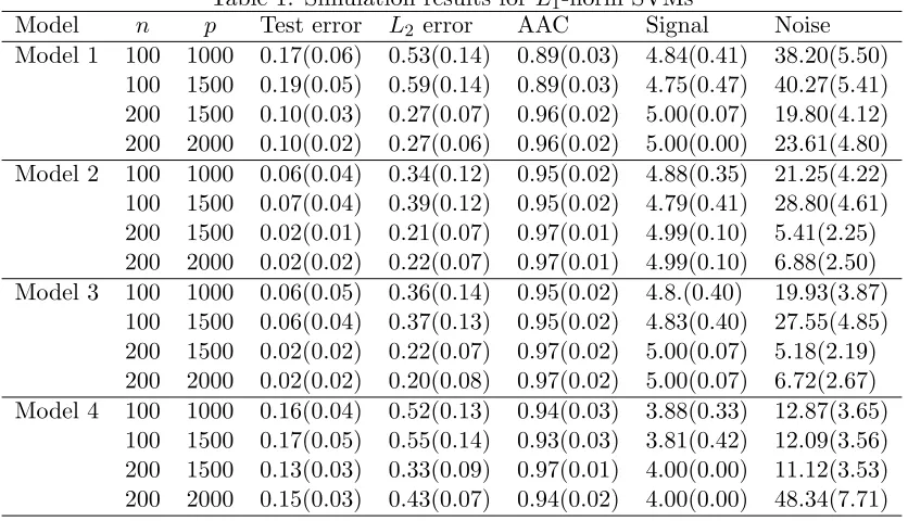
• Signal: the average of number of nonzero regression coefficients βbi 6= 0 with i = 1,2,3,4,5 for Model 1-3 and withi= 1,2,3,4 for Model 4. This measures the ability of L1-norm SVM selecting relevant features.
• Noise: the average of number of nonzero regression coefficients βbi(λ) 6= 0 with i6∈ {1,2,3,4,5} for Model 1-3 and with i 6∈ {1,2,3,4} for Model 4. This measures the ability ofL1-norm SVM not selecting noise features.
Table 1: Simulation results for L1-norm SVMs
Model n p Test error L2 error AAC Signal Noise
Model 1 100 1000 0.17(0.06) 0.53(0.14) 0.89(0.03) 4.84(0.41) 38.20(5.50) 100 1500 0.19(0.05) 0.59(0.14) 0.89(0.03) 4.75(0.47) 40.27(5.41) 200 1500 0.10(0.03) 0.27(0.07) 0.96(0.02) 5.00(0.07) 19.80(4.12) 200 2000 0.10(0.02) 0.27(0.06) 0.96(0.02) 5.00(0.00) 23.61(4.80) Model 2 100 1000 0.06(0.04) 0.34(0.12) 0.95(0.02) 4.88(0.35) 21.25(4.22) 100 1500 0.07(0.04) 0.39(0.12) 0.95(0.02) 4.79(0.41) 28.80(4.61) 200 1500 0.02(0.01) 0.21(0.07) 0.97(0.01) 4.99(0.10) 5.41(2.25) 200 2000 0.02(0.02) 0.22(0.07) 0.97(0.01) 4.99(0.10) 6.88(2.50) Model 3 100 1000 0.06(0.05) 0.36(0.14) 0.95(0.02) 4.8.(0.40) 19.93(3.87)
100 1500 0.06(0.04) 0.37(0.13) 0.95(0.02) 4.83(0.40) 27.55(4.85) 200 1500 0.02(0.02) 0.22(0.07) 0.97(0.02) 5.00(0.07) 5.18(2.19) 200 2000 0.02(0.02) 0.20(0.08) 0.97(0.02) 5.00(0.07) 6.72(2.67) Model 4 100 1000 0.16(0.04) 0.52(0.13) 0.94(0.03) 3.88(0.33) 12.87(3.65)
100 1500 0.17(0.05) 0.55(0.14) 0.93(0.03) 3.81(0.42) 12.09(3.56) 200 1500 0.13(0.03) 0.33(0.09) 0.97(0.01) 4.00(0.00) 11.12(3.53) 200 2000 0.15(0.03) 0.43(0.07) 0.94(0.02) 4.00(0.00) 48.34(7.71)
the models. Actually, the error rates are all quite close to the Bayes errors. It is also successful in eliminating most of the irrelevant features. The performance improves with increased sample size. In terms of estimation accuracy, theL2error decreases aspdecreases
and nincreases, which echoes the result in main theorem. We observe that AAC is greater than 0.9 in most cases, implying that the direction ofβb(λ) matches that of the Bayes rule. It is worth noting that the earlier literature have already performed thorough numerical analysis to compare the performance of L1-norm SVM with L2-norm SVM and logistic
regression. For example, Zhu et al. (2004) observes that the performance ofL1-norm SVM
andL2-norm SVM is similar when there is no redundant features; however, the performance
of L2-norm SVM can be adversely affected by the presence of redundant features. Rocha
et al. (2009) numerically compared L1-norm SVM with logistic regression classifier and
discovered that they are comparable but their relative finite-sample advantage depends on the sample size and design. See similar observation in Zou (2007), Zhang et al. (2016b), among others. Although L1-norm SVM can outperform regularL2-norm SVM when there
are many redundant features, it shares the drawback ofL1penalized least squares regression
that it overpenalizes large coefficients and tends to have larger false positives (including more noise features) comparing with the non-convex penalized SVM, which will be investigated in Section 5.2.
5.2 Monte Carlo results for non-convex penalized SVM
In this subsection, we consider the same four models as in Section 5.1. Instead of the L1-norm SVM, we use it as the initial value for the non-convex penalized SVM algorithm
functions: SCAD penalty (with a = 3.7) and MCP penalty (with a = 3). As suggested in Zhang et al. (2016b), we used the recently developed high-dimensional BIC criterion to choose the tuning parameter for non-convex penalized SVMs. More specifically, the SVM-extended BIC is defined as
SV M ICγ(T) = n X
i=1
2ξi+ log(n)|T|+ 2γ
p |T|
, 0≤γ ≤1,
where in practice we can setγ = 0.5 as suggested by Chen and Chen (2008) and choose the λthat minimizes the aboveSV M ICγ for non-convex penalized SVM.
Table 2: Simulation results for SCAD penalized SVM
Model n p Test error L2 error AAC Signal Noise
Model 1 100 1000 0.10(0.05) 0.25(0.17) 0.95(0.04) 4.88(0.38) 4.92(5.82) 100 1500 0.12(0.06) 0.35(0.20) 0.93(0.05) 4.84(0.53) 9.31(8.89) 200 1500 0.08(0.03) 0.15(0.10) 0.98(0.03) 4.99(0.12) 0.48(0.51) 200 2000 0.07(0.02) 0.10(0.05) 0.99(0.01) 5.00(0.00) 0.66(0.80) Model 2 100 1000 0.04(0.05) 0.25(0.17) 0.95(0.05) 4.73(0.51) 1.47(1.38) 100 1500 0.05(0.05) 0.28(0.18) 0.94(0.05) 4.64(0.55) 1.42(1.38) 200 1500 0.03(0.03) 0.19(0.10) 0.96(0.03) 4.91(0.29) 2.77(3.53) 200 2000 0.02(0.01) 0.15(0.06) 0.98(0.02) 5.00(0.07) 1.40(1.81) Model 3 100 1000 0.05(0.04) 0.30(0.16) 0.94(0.04) 4.53(0.58) 0.58(0.84) 100 1500 0.04(0.04) 0.24(0.15) 0.95(0.04) 4.75(0.46) 1.08(1.15) 200 1500 0.02(0.01) 0.14(0.06) 0.98(0.01) 4.99(0.10) 1.30(1.53) 200 2000 0.02(0.01) 0.15(0.06) 0.98(0.02) 5.00(0.00) 1.32(1.83) Model 4 100 1000 0.15(0.05) 0.51(0.20) 0.94(0.04) 3.50(0.59) 7.54(5.20) 100 1500 0.17(0.05) 0.61(0.18) 0.93(0.04) 3.57(0.71) 8.86(6.37) 200 1500 0.12(0.03) 0.19(0.10) 0.99(0.01) 3.98(0.14) 3.19(2.45) 200 2000 0.14(0.03) 0.39(0.19) 0.97(0.03) 3.69(0.51) 0.95(1.07)
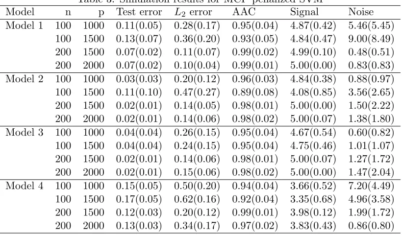
Tables 2 and 3 summarize the simulation results for SCAD and MCP penalty functions, respectively. We observe that the SCAD-penalized SVM and MCP-penalized MCP have similar performance, both demonstrating a clear advantage of selecting the relevant features and excluding irrelevant ones overL1-norm SVM. The Noise size decreases dramatically to
less than 3 as the sample size gets larger. The Signal size is almost 5 when n = 200 for Model 1-3 and 4 for Model 4, implying the success of selecting the exact true model. We also observe that non-convex penalized SVM has uniformly smallerL2error and larger AAC
thanL1-norm SVM. This resonates with the observation in the literature that eliminating
Table 3: Simulation results for MCP penalized SVM
Model n p Test error L2 error AAC Signal Noise
Model 1 100 1000 0.11(0.05) 0.28(0.17) 0.95(0.04) 4.87(0.42) 5.46(5.45) 100 1500 0.13(0.07) 0.36(0.20) 0.93(0.05) 4.84(0.47) 9.00(8.49) 200 1500 0.07(0.02) 0.11(0.07) 0.99(0.02) 4.99(0.10) 0.48(0.51) 200 2000 0.07(0.02) 0.10(0.04) 0.99(0.01) 5.00(0.00) 0.83(0.83) Model 2 100 1000 0.03(0.03) 0.20(0.12) 0.96(0.03) 4.84(0.38) 0.88(0.97) 100 1500 0.11(0.10) 0.47(0.27) 0.89(0.08) 4.08(0.85) 3.56(2.65) 200 1500 0.02(0.01) 0.14(0.05) 0.98(0.01) 5.00(0.00) 1.50(2.22) 200 2000 0.02(0.01) 0.14(0.06) 0.98(0.02) 5.00(0.07) 1.38(1.80) Model 3 100 1000 0.04(0.04) 0.26(0.15) 0.95(0.04) 4.67(0.54) 0.60(0.82) 100 1500 0.04(0.04) 0.24(0.15) 0.95(0.04) 4.75(0.46) 1.01(1.07) 200 1500 0.02(0.01) 0.14(0.06) 0.98(0.01) 5.00(0.07) 1.27(1.72) 200 2000 0.02(0.01) 0.15(0.06) 0.98(0.02) 5.00(0.00) 1.47(2.04) Model 4 100 1000 0.15(0.05) 0.50(0.20) 0.94(0.04) 3.66(0.52) 7.20(4.49) 100 1500 0.17(0.05) 0.62(0.16) 0.92(0.04) 3.35(0.68) 4.96(3.58) 200 1500 0.12(0.03) 0.20(0.12) 0.99(0.01) 3.98(0.12) 1.99(1.72) 200 2000 0.13(0.03) 0.34(0.17) 0.97(0.02) 3.83(0.43) 0.86(0.80)
6. Conclusion and discussion
We investigate the statistical properties ofL1-norm SVM coefficients in ultra-high
dimen-sion. We proved that L1-norm SVM coefficients achieve a near-oracle rate of estimation
error. To deal with the non-smoothness of the hinge loss function, we employ empirical processes techniques to derive the theory. Furthermore, we showed that under some general regularity conditions, theL1-norm SVM provides an appropriate initial value for the recent
algorithm developed by Zhang et al. (2016b) for non-convex penalized SVM in high dimen-sion. Combined with the theory in that paper, we extended the applicability and validity of their result to the ultra-high dimension.
Our work is motivated by the importance of identifying individual features for SVM in analyzing high-dimensional data, which frequently arise in genomics and many other fields. We not only closed a theoretical gap on the estimation error bound onL1-SVM whenpn,
but also verified that (Section 4) this leads to consistently identifying important features when combined with a two-step iterative algorithm in the ultra-high dimensional setting. Hence, we have guarantee for both algorithm convergence and theoretical performance. We believe such results are of direct interest to JMLR readers given the popularity of SVM in practice. Our work has substantial difference from the existing work in the literature. The existing theory on SVM has been largely focused on the analysis of generalization error rate and empirical risk. These results neither contain nor directly imply the transparent error bound of the estimated coefficients ofL1-norm SVM studied in this paper. Furthermore, the
techniques used in the paper for deriving the L2 error bound when p n are completely
different from those used in p < n setting. Although our approach for deriving the L2
new technical challenge to deal with the nonsmooth Hinge loss function and requires more delicate application of empirical process techniques. Also, unlike Lasso, we do not require Gaussian or sub-Gaussian conditions in the technical derivation.
Acknowledgments
We would like to acknowledge support for this project from the National Science Founda-tion (NSF grant DMS-1308960) for Peng and Wang’s research and the NaFounda-tional Science Foundation (NSF grant DMS-1055210) and National Institutes of Health (NIH grants R01 CA149569 and P01 CA142538) for Wu’s research respectively.
Appendix A: Technical Proofs
Proof of Lemma 1. By the union bound, we have
P cp2A(α) logp/n≤c||S(b β∗)||∞
≤ p X
j=0
Pp2A(α) logp/n≤n−1 n X
i=1
I(1−YiXTi β
∗ ≥0)Y
iXij
.
Notice that we have S(β∗) = 0 because of minimizer β∗ and the definition of gradient vector. Then, for each iand j,E(YiXijI(1−YiXTi β∗≥0)) = 0, by Hoeffding’s inequality,
Pp2A(α) logp/n≤n−1 n X
i=1
I(1−YiXTi β∗ ≥0)YiXij
≤ 2 exp(−4A(α)nlogp
4nM2 ) = 2p
−A(α)
M2 .
Terefore P cp2A(α) logp/n≤c||S(b β∗)||∞
≤(p+ 1)·2p−
A(α)
M2 ≤α.
Proof of Lemma 2. Sinceβbminimizesln(β), we have
1 n
n X
i=1
(1−YiXTi βb)++λ||bβ−||1 ≤ 1 n
n X
i=1
(1−YiXTi β∗)++λ||β∗−||1,
1 n
n X
i=1
(1−YiXTi β
∗+Y
iXTi h)+−
1 n
n X
i=1
(1−YiXTi β
∗)
+ ≤λ||β∗−||1−λ||bβ−||1.
RecallingT ={1≤j≤p:β∗j 6= 0}and T+=TS{0}, we have
||β∗−||1− ||βb−||1 ≤ ||β∗T
+||1− ||bβ−||1 ≤ ||hT+||1− ||hT+c||1. This implies
1 n
n X
i=1
(1−YiXTi β∗+YiXTi h)+−
1 n
n X
i=1
Since the subdifferential of ln(β) at the point of β∗ is S(b β∗) and recall the assumption λ≥c||S(b β∗)||∞, we have
1 n
n X
i=1
(1−YiXTi β∗+YiXTih)+−
1 n
n X
i=1
(1−YiXTi β∗)+
≥ SbT(β∗)h
≥ −||h||1· ||S(b β∗)||∞
≥ −λ
c(||hT+||1+||hT+c||1). Hence, we have
λ(||hT+||1− ||hT+c||1) ≥ − λ
c(||hT+||1+||hT+c||1), ||hT+||1 ≥ C||¯ hT+c||1,
where ¯C = cc−+11. We have thus proved that h∈∆C¯.
Proof of Lemma 3. We first consider a fixed h ∈ Rp+1 such that ||h||
0 ≤ q + 1 and
||h||26= 0. Note that the Hinge loss function is Lipschitz continuous and we have
(1−YiXTi β∗+YiXTi h)+−(1−YiXTi β∗)+
||h||2 ≤
|XTi h| ||h||2 . By Hoeffding’s inequality, we have ∀t >0,
P
B(h) ||h||2
≥ √t n
X
≤2 exp− 2nt
2
4||Xh||2 2/||h||22
.
Hence by assumption (A3),
P
B(h) ||h|| ≥
t √ n X
≤2 exp− t
2
2λmax
≤2 exp− t
2
2M1
.
Lett=C√2qlogp, where C is an arbitrary given positive constant. Then
PB(h) ||h|| ≥C
r
2qlogp n
≤ 2 exp−C
2qlogp
M1
≤2p−C2q/M1 ≤2p−C2(q+1)/(2M1).
Next we will derive an upper bound for sup
||h||0≤q+1,||h||26=0
B(h)
||h||. We consider covering {h ∈
Rp+1,||h||0 ≤ q+ 1} with -balls such that for any h1 and h2 in the same ball we have
||hh1
1||2 −
h2
||h2||2
≤ , where is a small positive number. The number of -balls that is
required to cover a k-dimensional unit ball is bounded by (3/)k, see for example Rogers (1963) and Bourgain and Milman (1987). Since h is a (p+ 1)-dimensional vector with at mostq+1 nonzero coordinates andh/||h||2has unit length inL2norm, the covering number
we require is at most (3p/)q+1. LetN denote such an -net. By the union bound,
P sup
h∈N
B(h) ||h||2
≥C r
2qlogp n ! ≤2 3p q+1
p−C2(q+1)/(2M1)= 2
3
p
for any given positive constant C. Furthermore, for any h1,h2 ∈Rp+1 such that ||h1||0 ≤
q+ 1,||h2||0≤q+ 1, ||h1||26= 0 and ||h2||26= 0, we have
B(h1)
||h1||2
−B(h2) ||h2||2
≤
2
n||X h1/||h1||2−h2/||h2||2
||1 ≤ √2
n||X h1/||h1||2−h2/||h2||2
||2 ≤ 2pM1.
Therefore,
sup
||h||0≤q+1,||h||26=0 B(h)
||h|| ≤hsup∈N B(h)
||h|| + 2 p
M1.
Let= q
qlogp
2M1n, we have
P sup
||h||0≤q+1,||h||26=0 B(h) ||h||2
≥C r
2qlogp n
!
≤ P sup
h∈N
B(h) ||h||2
≥(C−1) r
2qlogp n
!
≤ 2 2M1n qlogp
q+12
3p1−(C−1)2/(2M1)q+1 ≤ 2 p2M1n3p1−(C−1)
2/(2M 1)q+1. Since p > n, takeC= 1 + 2C1
√
M1 for someC1>1, then for allnsufficiently large,
P sup
||h||0≤q+1,||h||26=0 B(h)
||h|| ≥(1 + 2C1 p
M1)
r
2qlogp n
≤2p−2q(C12−1).
Lemma 6 For any x∈Rn,
||x||2−
||x||√ 1
n ≤
√ n
4 1max≤i≤n|xi| −1min≤i≤n|xi ).
Proof. This proof was given in Cai, Wang, and Xu (2010). We include it here for complete-ness and easy reference. It is obvious that the result holds when |x1|=|x2|= . . .= |xn|.
Without loss of generality, we now assume that x1 ≥x2 ≥. . .≥xn ≥0 and not allxi are
equal. Let
f(x) =||x||2− ||x||√ 1 n .
Note that for any i∈ {2,3, . . . , n−1}
∂f ∂xi
= xi
||x||2 − 1 √
This implies that whenxi ≤ ||√x||2
n ,f(x) is decreasing w.r.txi; otherwise f(x) is increasing w.r.t xi. Hence, if we fix x1 and xn, when f(x) achieves its maximum, x must be of the form thatx1 =x2=. . .=xk and xk+1 =. . .=xn for some 1≤k≤n. Now,
f(x) = q
k(x2
1−x2n) +nx2n− k √
n(x1−xn)− √
nxn.
Treat this as a function ofk fork∈(0, n).
g(x) = q
k(x21−x2
n) +nx2n−
k √
n(x1−xn)− √
nxn.
By taking the derivatives, it is easy to see that
g(k) ≤ g n(
x1+xn
2 ) 2−x2
n x21−x2
n !
= √n(x1−xn)
1 2−
x1+ 3xn 4(x1+xn)
.
Since 12− x1+3xn 4(x1+xn) ≥
1
4, we have
||x||2 ≤ ||x||√ 1
n +
√ n
4 (x1−xn).
We can also see that the above inequality becomes an equality if and only if xk+1 =. . .=
xn= 0 and k= n4.
Proof of Theorem 4. Leth=β∗−βb, then it follows from Lemma 2 thath∈∆C¯. Assume
without loss of generality that|h0| ≥ |h1| ≥. . .≥ |hp|. Create a partition of{0,1,2, . . . , p}
as
S0 ={0,1,2, . . . , q}, S1 ={q+ 1, q+ 2. . . ,2q+ 1}, S2 ={2q+ 2,2q+ 3. . . ,3q+ 2}, . . .
where Si,i= 1,2, . . ., has cardinality q+1, except the last set which may have cardinality smaller than q+1. This partition leads to the following decomposition
1 n
n X
i=1
(1−YiXTi β∗+YiXTi h)+−
1 n
n X
i=1
(1−YiXTiβ∗)+
= 1
n n X
i=1
(1−YiXTi β∗+YiXTi X
k≥0
hSk)+−
1 n
n X
i=1
(1−YiXTi β∗)+
= X
j≥1
1 n
n X
i=1
(1−YiXTi β∗+YiXTi
j X
k=0
hSk)+−
n X
i=1
(1−YiXTi β∗+YiXTi
j−1
X
k=0
hSk)+
! +1 n n X i=1
(1−YiXTi β∗+YiXTi hS0)+− n X
i=1
(1−YiXTi β∗)+
!
where the first equation follows from the definition ofhSk,k≥0; the second equation holds
by observing that the intermediate terms cancel out each other. The purpose of the above decomposition is to obtain more accurate probability bounds by appealing to Lemma 3. This is made possible by noting that the jth term in the sum of the above decomposition has the increment indexed by hSj, which has at most q+1 nonzero coordinates. Lemma 3
implies that uniformly for j= 1,2, . . ., with probability at least 1−2p−2q(C12−1), 1
n n X
i=1
(1−YiXTiβ∗+YiXTi j X
k=0
hSk)+−
n X
i=1
(1−YiXTi β∗+YiXTi
j−1
X
k=0
hSk)+
! ≥ 1 nE n X i=1
(1−YiXTiβ∗+YiXTi
j X
k=0
hSk)+−
n X
i=1
(1−YiXTiβ∗+YiXTi
j−1
X
k=0
hSk)+
!
−C r
2qlogp
n ||hSj||2,
whereC = 1 + 2C1
√
M1. Hence by (16), with probability at least 1−2p−2q(C
2 1−1), 1
n
Xn
i=1
(1−YiXTi β∗+YiXTi h)+−
n X
i=1
(1−YiXTi β∗)+
≥M(h)−C r
2qlogp n
X
j≥0
||hSj||2
(17)
whereM(h) = 1nE(Pni=1(1−YiXTiβ∗+YiXTi h)+−Pni=1(1−YiXTi β∗)+).
It is straightforward to show that ||hS0||1 ≥ ||hT+||1 ≥ C||¯ hTC
+||1 ≥ ¯ C||hSC
0||1. By Lemma 6, we have
X
j≥1
||hSj||2 ≤
X
j≥1
||hSj||1
√
q+ 1 + √
q+ 1 4 |hq|
≤ ||√hS0C||1 q+ 1 +
||hS0||1 4√q+ 1
≤ √ 1
q+ 1 ¯C + 1 4√q+ 1
||hS0||1
≤ 1 4 + 1 ¯ C
||hS0||2. (18)
By the definition ofh, (15), (17) and (18), we have
M(h) ≤ λ(||hT+||1− ||hTC
+||1) + 1 4 + 1 ¯ C C r
2qlogp
n ||hS0||2+C r
2qlogp
n ||hS0||2 ≤ λpq+ 1||hS0||2+C
r
2qlogp n 5 4 + 1 ¯ C
||hS0||2. (19)
Condition (A4) imply that
M(h) = 1 2h
TH(β∗)h+o(||h||2
2)≥
1
2M2||h||
2
Combining (19) and (20), we have
1
2M2||h||
2
2+o(||h||22) ≤ λ
p
q+ 1||hS0||2+C r
2qlogp n 5 4 + 1 ¯ C
||hS0||2. Note that||h||2
2=||hS0||
2 2+
P
j≥1||hSj||
2
2≥ ||hS0||
2 2, and
X
j≥1
||hSj|| 2
2 ≤ |hq|
X
j≥1
||hSj||1 ≤
1 ¯
C|hq|||hS0||1 ≤ 1
¯ C||hS0||
2 2.
So ||h||2
2 ≤(1 + C1¯)||hS0||
2
2. This implies o(||h||22) =o(||hS0||
2
2). To wrap up, we have
||hS0||2+o(||hS0||2)≤
2λ√q+ 1 M2
+ 2C
M2
r
2qlogp n 5 4 + 1 ¯ C . Hence,
||h||2+o(||h||2)≤ r
1 + 1¯ C
2λ√q+ 1 M2
+ 2C M2
r
2qlogp n 5 4 + 1 ¯ C ! .
We therefore have
||βb−β∗||2 ≤ r
1 + 1¯ C
2λ
√ q+ 1 M2
+ 2C M2
r
2qlogp n 5 4+ 1 ¯ C
with probability at least 1−2p−2q(C12−1).
Proof of Theorem 5. It follows by combining the result of Theorem 3.3 with that of Theorem 4 in of Zhang et al. (2016b).
Appendix B: Discussions of Condition (A4)
We note that Condition (A4) is satisfied if the smallest eigenvalues of H(β∗) has a positive lower bound. In the following, we provide a set of sufficient conditions to guarantee the positive definiteness of H(β∗).
(A1∗) For some 1≤k≤p,
Z
S
I(Xk≥Vk−)Xig(X)dX< Z
S
I(Xk ≤Uk+)Xif(X)dX or
Z
S
I(Xk≤Vk+)Xig(X)dX> Z
S
I(Xk ≥Uk−)Xif(X)dX
Here Uk+, Vk+ ∈ [−∞,+∞] are upper bounds such that R
SI(Xk ≤ Uk+)f(X)dX = min(1,π−
π+) and R
SI(Xk ≤ V
+
k )f(X)dX = min(1,
π+
π−). Similarly, lower bounds U
−
k,
Vk− ∈ [−∞,+∞] and are defined as R
SI(Xk ≥ U −
k)f(X)dX = min(1,
π−
π+) and R
SI(Xk≥V −
k )g(X)dX= min(1,
π+
(A2∗) For an orthogonal transformation Aj that maps
β∗−
||β∗−||2
to thej-th unit vector ej for
somej∈ {1,2,3, . . . , p}, there exists rectangles
D+={x∈M+:li ≤(Ajx)i ≤vi with li< vi fori6=j} and
D−={x∈M−:li ≤(Ajx)i ≤vi with li< vi fori6=j}
such that f(x) ≥ B1 > 0 on D+, and g(x) ≥ B2 > 0 on D−, where M+ = {x ∈ Rp|xTβ∗
−+β∗0 = 1} and M−={x∈Rp|xTβ
∗
−+β∗0 =−1}.
Also with some technical modification, Condition (A1) in our paper can be further relaxed to
(A3∗) The densities f and g are continuous with common support S ⊂ Rp and have finite second moments.
As an interesting side result, Lemma 5 in Koo et al. (2008) showed that Condition (A4) holds under (A1∗)-(A3∗). Although their paper’s results on the Bahadur representation of L1-norm SVM coefficients are restricted to the classical fixed p case, a careful examination
of the derivation showed that this particular lemma holds irrespective of the dimension of p.
In the following, we demonstrate that Conditions (A1∗)-(A3∗) hold in a nontrivial exam-ple where we have two multivariate normal distributions inRp. The marginal distribution of Y is given byπ+=π−= 1/2. Letf and gbe the density functions ofX− givenY = 1 and
−1, respectively. Here, we assumef and g are multivariate normal densities with different mean vectors µand ν and a common covariance matrix Σ. This setup was also considered in Koo et al. (2008) but we will provide more details to show condition (A4) is satisfied in our high-dimensional setting. In particular, we will provide some details for deriving the analytic forms ofβ∗ and H(β∗), which complements the results in Koo et al. (2008).
For normal density functions f andg, it is straightforward to check Condition (A3∗) is satisfied. WhileUk+ =Vk+= +∞ andUk− =Vk− =−∞, Condition (A1∗) also holds. Since D+andD−are bounded rectangles inRp, the normal densitiesf andgare always bounded
away from zero onD+andD−. Thus (A2∗) is satisfied. Denote the density and cumulative distribution function of standard normal distributionN(0,1) asφand Φ, respectively. Then we have S(β∗) = 0, whereS(·) is defined in (6), that is
Ef(I(1−XTβ∗≥0)) =Eg(I(1 +XTβ∗≥0)) (21)
and
Ef(I(1−XTβ∗ ≥0)X−) =Eg(I(1 +XTβ∗≥0)X−) (22)
For left hand of equation (21), we haveXT
−β∗− ∼N(µTβ−∗,β∗−TΣβ∗−), thus
Ef(I(1−XTβ∗≥0)) =Pf(1−β0∗−XT−β∗−≥0) = Φ(cf), (23) wherecf =
1−β0∗−µTβ
∗ −
||Σ1/2
β∗−||2
. Similarly,Eg(I(1 +XTβ∗≥0)) = Φ(cg). wherecg = 1+β
∗
0+νTβ
∗ −
||Σ1/2
To obtain an analytic expression of Ef(I(1−XTβ∗ ≥ 0)), we consider an
orthogo-nal matrix P that satisfies PΣ 1/2
β∗−
||Σ1/2β∗−||2
= (1,0,0, . . . ,0)T. Such a matrix P can always
be constructed. Actually, let P = (P1,P2, . . . ,Pp)T and P1 = Σ 1/2
β∗−
||Σ1/2β∗−||2
. By using
Gram-Schmidt process, we can generate other orthogonal vectors Pi based on P1 with i= 2,3, . . . , p. SincePΣ−1/2(X−−µ) =Z, a standard multivariate normal random vector,
we have I−XTβ∗=cf||Σ1/2β∗−||2−ZTPΣ1/2β∗−. Thus
Ef(I(1−XTβ∗ ≥0)X−) = Eφ(I(cf −Z1 ≥0)(Σ1/2PTZ+µ))
= Eφ(I(cf −Z1 ≥0)µ) +Eφ(I(cf−Z1 ≥0)Σ1/2PTZ).
where φis the joint probability density function of a p-dimensional standard multivariate normal distribution. We will compute the above expectation componentwise. Let Σ1/2 = Λ = (Λ1,Λ2, . . . ,Λp)T. Fork= 1, . . . , p, we have
Ef(I(1−XTβ∗ ≥0)Xk) = µkΦ(cf) +Eφ I(cf −Z1 ≥0)ΛTk p X
i=1
PiZi
where. SinceZ2, . . . , Zp have mean zero and are independent ofZ1,
Eφ I(cf−Z1≥0)ΛTk p X
i=1
(PiZi)
= Eφ I(cf −Z1≥0)ΛTkP1Z1
= ΛTk Σ
1/2β∗ −
||Σ1/2β∗−||2Eφ I(cf −Z1 ≥0)Z1
= ΛTk Σ
1/2β∗ −
||Σ1/2β∗−||2
Z +∞
−∞
I cf −x≥0xφ(x)dx
= ΛTk Σ
1/2β∗ −
||Σ1/2β∗−||2 Z cf
−∞
xφ(x)dx
Since xφ(x) is an odd function andφ(x) is symmetric, we have
Z cf
−∞
xφ(x)dx =
Z |cf|
−∞
xφ(x)dx=−√1 2π
Z +∞
c2
f
1 2exp(−
z
2)dz=−φ(cf).
Therefore, fork= 1, . . . , p,Ef I(1−XTβ∗ ≥0)Xk
=µkΦ(cf)−ΛTk
Σ1/2β∗−
||Σ1/2β∗−||2
φ(cf).Hence
Ef(I(1−XTβ∗ ≥0)X−) =µΦ(cf)−φ(cf)Σ1/2P1.
Similarly,
Then, we have
Φ(cf) = Φ(cg) (24)
and
µΦ(cf)−φ(cf)Σ1/2P1 =νΦ(cg) +φ(cg)Σ1/2P1 (25) From (24), we have ˜c=cf =cg, which implies
β∗−T(µ+ν) =−2β0∗ (26)
From (25),
β∗−
||Σ1/2β∗−||2 = Φ(˜c) 2φ(˜c)Σ
−1(µ−ν) (27)
LetdΣ(µ,ν) = ((µ−ν)TΣ−1(µ−ν))1/2 be the Mahalanobis distance betweenµandν and
R(x) = Φ(φ(xx)). AsΣ1/2 β
∗ −
||Σ1/2β∗−||2
hasl2 norm equal to 1, we have||2Φ(˜φ(˜cc))Σ−1/2(µ−ν)||2 = 1, i.e., R(˜c) = dΣ(µ,ν)
2 . R(x) is a monotonically decreasing function, thus we have ˜c =
R−1 dΣ(µ,ν)
2
. Meanwhile, ˜c =cf = 1−β
∗
0−µTβ
∗ −
||Σ1/2β∗−||2
, we can solve the problem based on (26)
and (27),
β0∗ =−(µ−ν)
TΣ−1(µ+ν)
2˜cdΣ(µ,ν) +d2Σ(µ,ν)
(28)
From (25),
β∗− = 2Σ
−1(µ−ν)
2˜cdΣ(µ,ν) +d2Σ(µ,ν)
(29)
By plugging (28) and (29) into (7), we can calculateH(β∗) as
H(β∗) = φ(˜c)
4 (2˜c+dΣ(µ,ν))
2 (µ+ν)T
µ+ν H22(β∗)
(30)
where
H22(β∗) =µµT +ννT + 2Σ+ 2
˜ c dΣ(µ,ν)
2
+ c˜
dΣ(µ,ν)
− 1
d2 Σ(µ,ν)
!
(µ−ν)(µ−ν)T
As we have obtained the analytic form of H(β∗), we consider Model 1 in Section 5.1 as an example. In Model 1, q = 5, µ = (0.1,0.2,0.3,0.4,0.5,0, . . . ,0)T and ν = (−0.1,−0.2,−0.3,−0.4,−0.5,0, . . . ,0)T ∈ Rp and π+ = π− = 1/2. The covariance
References
Natalia Becker, Grischa Toedt, Peter Lichter, and Axel Benner. Elastic scad as a novel penalization method for svm classification tasks in high-dimensional data. BMC bioin-formatics, 12(1):138, 2011.
Alexandre Belloni and Victor Chernozhukov. l1-penalized quantile regression in
high-dimensional sparse models. The Annals of Statistics, 39(1):82–130, 2011.
Peter J Bickel, Ya’acov Ritov, and Alexandre B Tsybakov. Simultaneous analysis of lasso and dantzig selector. The Annals of Statistics, 37(4):1705–1732, 2009.
Bernhard E Boser, Isabelle M Guyon, and Vladimir N Vapnik. A training algorithm for optimal margin classifiers. InProceedings of the Fifth Annual Workshop on Computational Learning Theory, pages 144–152. ACM, 1992.
Jean Bourgain and Vitaly D Milman. New volume ratio properties for convex symmetric bodies inRn. Inventiones Mathematicae, 88(2):319–340, 1987.
Paul S Bradley and Olvi L Mangasarian. Feature selection via concave minimization and support vector machines. InICML, volume 98, pages 82–90, 1998.
Tony Cai, Lie Wang, and Guangwu Xu. New bounds for restricted isometry constants.
IEEE Transactions on Information Theory, 56(9):4388–4394, 2010.
Tony Cai, Weidong Liu, and Xi Luo. A constrained l1 minimization approach to sparse
precision matrix estimation. Journal of the American Statistical Association, 106(494): 594–607, 2011.
Yin-Wen Chang and Chih-Jen Lin. Feature ranking using linear svm. Causation and Prediction Challenge Challenges in Machine Learning, 2:47, 2008.
Jiahua Chen and Zehua Chen. Extended bayesian information criteria for model selection with large model spaces. Biometrika, 95(3):759–771, 2008.
R Dennis Cook, Bing Li, and Francesca Chiaromonte. Dimension reduction in regression without matrix inversion. Biometrika, 94(3):569–584, 2007.
Jianqing Fan and Runze Li. Variable selection via nonconcave penalized likelihood and its oracle properties. Journal of the American statistical Association, 96(456):1348–1360, 2001.
Eitan Greenshtein et al. Best subset selection, persistence in high-dimensional statistical learning and optimization under l1 constraint. The Annals of Statistics, 34(5):2367–2386, 2006.
Ja-Yong Koo, Yoonkyung Lee, Yuwon Kim, and Changyi Park. A bahadur representation of the linear support vector machine. The Journal of Machine Learning Research, 9: 1343–1368, 2008.
Yi Lin. Support vector machines and the bayes rule in classification. Data Mining and Knowledge Discovery, 6(3):259–275, 2002.
Nicolai Meinshausen and Bin Yu. Lasso-type recovery of sparse representations for high-dimensional data. The Annals of Statistics, pages 246–270, 2009.
Changyi Park, Kwang-Rae Kim, Rangmi Myung, and Ja-Yong Koo. Oracle properties of scad-penalized support vector machine. Journal of Statistical Planning and Inference, 142(8):2257–2270, 2012.
Guilherme V Rocha, Xing Wang, and Bin Yu. Asymptotic distribution and sparsistency for l1-penalized parametric m-estimators with applications to linear svm and logistic regression. arXiv preprint arXiv:0908.1940, 2009.
CA Rogers. Covering a sphere with spheres. Mathematika, 10(02):157–164, 1963.
Minghu Song, Curt M Breneman, Jinbo Bi, Nagamani Sukumar, Kristin P Bennett, Steven Cramer, and Nihal Tugcu. Prediction of protein retention times in anion-exchange chro-matography systems using support vector regression. Journal of Chemical Information and Computer Sciences, 42(6):1347–1357, 2002.
Bernadetta Tarigan and Sara Anna van de Geer. Adaptivity of Support Vector Machines with L1 Penalty. University of Leiden. Mathematical Institute, 2004.
Bernadetta Tarigan, Sara A Van De Geer, et al. Classifiers of support vector machine type with l1 complexity regularization. Bernoulli, 12(6):1045–1076, 2006.
Sara A Van de Geer. High-dimensional generalized linear models and the lasso. The Annals of Statistics, 36(2):614–645, 2008.
Vladimir Vapnik. The Nature of Statistical Learning Theory. Springer Science & Business Media, 1995.
Lan Wang, Yichao Wu, and Runze Li. Quantile regression for analyzing heterogeneity in ultra-high dimension. Journal of the American Statistical Association, 107(497):214–222, 2012.
Lie Wang. The l1 penalized lad estimator for high dimensional linear regression. Journal of Multivariate Analysis, 120:135–151, 2013.
Lifeng Wang and Xiaotong Shen. Onl1-norm multiclass support vector machines:
method-ology and theory. Journal of the American Statistical Association, 102(478):583–594, 2007.
Cun-Hui Zhang. Nearly unbiased variable selection under minimax concave penalty. The Annals of Statistics, 38(2):894–942, 2010.
Hao Helen Zhang, Jeongyoun Ahn, Xiaodong Lin, and Cheolwoo Park. Gene selection using support vector machines with non-convex penalty. Bioinformatics, 22(1):88–95, 2006.
Xiang Zhang, Yichao Wu, Lan Wang, and Runze Li. A consistent information criterion for support vector machines in diverging model spaces. Journal of Machine Learning Research, 17(16):1–26, 2016a.
Xiang Zhang, Yichao Wu, Lan Wang, and Runze Li. Variable selection for support vector machines in moderately high dimensions. Journal of the Royal Statistical Society: Series B (Statistical Methodology), 78(1):53–76, 2016b.
Ji Zhu, Saharon Rosset, Trevor Hastie, and Rob Tibshirani. 1-norm support vector ma-chines. Advances in Neural Information Processing Systems, 16(1):49–56, 2004.
Hui Zou. An improved 1-norm svm for simultaneous classification and variable selection.